Generalized models as a universal approach to the analysis of nonlinear dynamical systems

Abstract

We present a universal approach to the investigation of the dynamics in generalized models. In these models the processes that are taken into account are not restricted to specific functional forms. Therefore a single generalized models can describe a class of systems which share a similar structure. Despite this generality, the proposed approach allows us to study the dynamical properties of generalized models efficiently in the framework of local bifurcation theory. The approach is based on a normalization procedure that is used to identify natural parameters of the system. The Jacobian in a steady state is then derived as a function of these parameters. The analytical computation of local bifurcations using computer algebra reveals conditions for the local asymptotic stability of steady states and provides certain insights on the global dynamics of the system. The proposed approach yields a close connection between modelling and nonlinear dynamics. We illustrate the investigation of generalized models by considering examples from three different disciplines of science: a socio-economic model of dynastic cycles in china, a model for a coupled laser system and a general ecological food web.

I Introduction

Dynamical systems are used to study phenomena from diverse disciplines of science such as laser physics, population ecology, socio-economic studies and many more. The corresponding mathematical models have often the form of balance equations, in which the time evolution of the state variables is determined by gain and loss terms. Depending on the processes that are taken into account, a single state variable can be effected by several gains and losses. In the modeling process the modeler usually decides first which processes are important and need to be included in the model. These processes determine the structure of the model. In the second step each of the terms is described by a specific mathematical function, which can be based on theoretical reasoning or empirical evidence. In this way a specific model for the phenomenon under consideration is constructed. The investigation of specific models is a powerful approach, that has, in many cases, revealed interesting insights. However, the specific mathematical functions on which these models are based depend critically on the modelers knowledge of the system. While the modeler may have much information about certain processes, others may be known or believed to exist which are very difficult to quantify.

Specific models are therefore often based on a large number of assumptions. This can be illustrated very well by considering an example from ecology: The so-called Holling type-II function is regularly used to describe the predator-prey interaction in food webs and food chainsHolling (1959). This function takes major biological effects into account. But, it can not possibly capture all the subtle biological details that exist in nature. Such details may involve the formation of swarms to confuse predators, adaptation of the prey to high predator densities, density dependent changes in the predator’s foraging strategy to name a few. In models such details are often omitted on purpose since the modeler is interested in general insights that do not depend on specific properties of the system under consideration. But on the other hand, certain details may have a strong impact on the qualitative behavior of the system. For instance, it has been shown that even minor variations in the functional form of the predator-prey interaction can have a strong impact on the system’s stability Gross et al. (2004); Fussmann and Blasius (2005).

In contrast to specific functional forms, the basic structure of the system is much easier to determine. For instance in our ecological example it is easier to say that the predation depends on the population density of predator and prey than to derive the exact functional form that quantifies this dependence. It can therefore be useful to consider generalized models which describe the structure of a system in terms of gains and losses but do not restrict these processes to specific functional forms. If a system is considered in which some processes are known with a high degree of certainty while others remain uncertain it can be useful to study partially generalized models in which some processes are described by specific functional forms, while others remain general. In other cases fully generalized models in which all processes are modeled by generalized functions can be advantageous. Generalized models describe systems with a higher generality than specific models. They depend on less assumptions and enable the researcher to consider the system from an abstract point of view.

Despite the generality of generalized models, it is possible to compute the stability of a steady state in these models analytically. This reveals the exact relationship between the qualitative features of functional forms and the local bifurcations of steady states Gross et al. (2004). In this way the application of generalized models enables us to investigate the local stability of systems with a high degree of generality. Moreover, we can draw certain conclusions on the global dynamics of the system under consideration. For instance, the presence of chaotic or quasiperiodic dynamics as well as the existence of homoclinic bifurcations can be deduced form certain local bifurcations of higher codimension. In this way the presence of chaotic dynamics can be shown for a whole class of model systems Gross et al. (2005).

In this paper we present a universal approach to the investigation of generalized models based on balance equations. We illustrate this approach using three models from three different fields of science: socio-economics, laser physics and population dynamics. These examples demonstrate that the proposed approach can be used to study a wide range of systems.

The paper is organised as follows. We introduce our approach by considering a simple socio-economic model in Sec. II. The underlying principles of the normalization procedure are discussed in more detail while we study a coupled laser system in Sec. III. Finally, we show that the proposed approach is applicable to more involved problems by investigating a model for general food webs in Sec. IV.

II A generalized model of dynastic cycles

Chinese history is characterised by repeated transitions from despotism to anarchy and back Usher (1989). This periodic behavior is known as the dynastic cycle. As a young dynasty rises from anarchy a period of order and prosperity begins. As a result the population grows. At some point the aging dynasty can not control the growing population any longer. The results are poverty, crime and civil war which lead back to a period of anarchy. By contrast, European dynasties exhibit stable behavior for extended periods of time.

It has been shown in Usher (1989) that the existence of dynastic cycles as well as steady state behavior (e.g. stable dynasties) can be predicted by a simple three-variable model that describes the evolution of a society of farmers $X$, bandits $Y$ and rulers $Z$. The dynamics of this model have been investigated in Feichtinger et al. (1974). In these investigations a specific model was used in which the interactions between the different social groups were described by specific functions. In the following we study a generalized version of this model in which the interactions are described by general functions.

II.1 Formulation of a generalized model of dynastic cycles

In the model the growth of the population of farmers is described by a function $S(X)$. This function represents agricultural production, but also losses because of natural mortality including diseases. The population of farmers is reduced by crime $C(X,Y)$ and taxes $T(X,Z)$. Since the bandits profit from the crime their number is assumed to increase proportional to $C(X,Y)$. In addition crime increases the willingness of the farmers to support rulers. Therefore the number of rulers also grows proportional to $C(X,Y)$. The rulers fight crime by reducing the number of bandits. This effect of the rulers on the bandit population is described by a function $L(Y,Z)$. Finally, we take into account that the numbers of rulers and bandits decrease because of retirement and natural mortality. This loss is denoted by $M(Y)$ for the bandits and $R(Z)$ for the rulers. Taking all these factors into account one obtains differential equations of the form

$$\begin{array}[]{r c l}\dot{X}&=&S(X)-C(X,Y)-T(X,Z),\\ \dot{Y}&=&\eta C(X,Y)-L(Y,Z)-M(Y),\\ \dot{Z}&=&\nu C(X,Y)-R(Z)\end{array}$$ (1)

where $\eta$ and $\nu$ are constant factors.

II.2 Normalization of the socio-economic model

So far we have formulated a generalized version of the model proposed in Usher (1989). In general the investigation of such a model would start with the computation of steady states. However, in our model we can not compute steady states with the chosen degree of generality. Instead, we assume that at least one steady state exists. This assumption is in general valid in a large parameter range. We denote the population densities in this steady state by $X^{*}$, $Y^{*}$ and $Z^{*}$ respectively.

Let us now consider the local asymptotic stability of the steady state under consideration. In a system of autonomous ordinary differential equations (ODEs), such as Eq. (1), the stability of steady states depends on the eigenvalues of the corresponding Jacobian matrix Guckenheimer and Holmes (2002). For any system ODEs of the form $\dot{\rm\bf x}={\rm\bf g}({\rm\bf x})$ the Jacobian ${\rm\bf J}$ can be computed as

$$J_{m,n}=\left.\frac{\partial g_{m}}{\partial x_{n}}\right|_{\rm\bf x=x^{*}}\hskip 28.45274ptm,n=1,\ldots,N.$$ (2)

In principle we could therefore compute the Jacobian of our system directly by applying this definition to the system from Eq. (1). However, the Jacobian obtained in this way would depend explicitly on the unknown steady state. Because of this dependence the interpretation of any insights gained from such a Jacobian is difficult. In order to avoid this difficulty we study a normalized system. By means of normalization it possible to arrive at a system for which the Jacobian does not depend explicitly on the unknown steady state. Instead, the unknown steady state only appears in certain parameters which are easily interpretable.

In the following we use the abbreviated notation

$$\begin{array}[]{r c l r c l}S^{*}&:=&S(X^{*}),C^{*}&:=&C(X^{*},Y^{*}),\\ T^{*}&:=&T(X^{*},Z^{*}),L^{*}&:=&L(Y^{*},Z^{*}),\\ M^{*}&:=&M(Y^{*}),R^{*}&:=&R(Z^{*}).\end{array}$$ (3)

Using this notation, we define normalized state variables

$$x\displaystyle=\displaystyle\frac{\displaystyle X}{\displaystyle X^{*}},\displaystyle y\displaystyle=\displaystyle\frac{\displaystyle Y}{\displaystyle Y^{*}},\displaystyle z\displaystyle=\displaystyle\frac{\displaystyle Z}{\displaystyle Z^{*}}$$ (4)

and normalized functions

$$\begin{array}[]{r c l}\displaystyle s(x)&:=&\displaystyle\frac{S(X^{*}x)}{S^{*}},\\[5.0pt] \displaystyle c(x,y)&:=&\displaystyle\frac{C(X^{*}x,Y^{*}y)}{C^{*}},\\[5.0pt] \displaystyle t(x,z)&:=&\displaystyle\frac{T(X^{*}x,Z^{*}z)}{T^{*}},\\[5.0pt] \displaystyle l(y,z)&:=&\displaystyle\frac{L(Y^{*}y,Z^{*}z)}{L^{*}},\\[5.0pt] \displaystyle m(y)&:=&\displaystyle\frac{M(Y^{*}y)}{M^{*}},\\[5.0pt] \displaystyle r(z)&:=&\displaystyle\frac{R(Z^{*}z)}{R^{*}}.\end{array}$$ (5)

Note that the normalized quantities have been defined in such a way that

$$x^{*}=y^{*}=z^{*}=s^{*}=c^{*}=t^{*}=l^{*}=m^{*}=r^{*}=1$$ (6)

holds.

Let us now rewrite our model in terms of the normalized variables. We start by substituting the definitions Eq. (4) and Eq. (5) into Eq. (1). We obtain

$$\begin{array}[]{r c l}\dot{x}&=&\displaystyle\frac{S^{*}}{X^{*}}s(x)-\frac{C^{*}}{X^{*}}c(x,y)-\frac{T^{*}}{X^{*}}t(x,z),\\[5.0pt] \dot{y}&=&\displaystyle\frac{\eta C^{*}}{Y^{*}}c(x,y)-\frac{L^{*}}{Y^{*}}l(y,z)-\frac{M^{*}}{Y^{*}}m(y),\\[5.0pt] \dot{z}&=&\displaystyle\frac{\nu C^{*}}{Z^{*}}c(x,y)-\frac{R^{*}}{Z^{*}}r(z).\end{array}$$ (7)

In order to simplify these equations we consider the system in the steady state. Because of Eq. (6) this yields

$$\begin{array}[]{r c l}0&=&\displaystyle\frac{S^{*}}{X^{*}}-\frac{C^{*}}{X^{*}}-\frac{T^{*}}{X^{*}},\\[5.0pt] 0&=&\displaystyle\frac{\eta C^{*}}{Y^{*}}-\frac{L^{*}}{Y^{*}}-\frac{M^{*}}{Y^{*}},\\[5.0pt] 0&=&\displaystyle\frac{\nu C^{*}}{Z^{*}}-\frac{R^{*}}{Z^{*}}.\end{array}$$ (8)

Since Eq. (8) contains only constants the equation has to hold even if the system is in a non-stationary state. It is therefore reasonable to define

$$\begin{array}[]{r c l}\alpha_{\rm x}&=&\displaystyle\frac{S^{*}}{X^{*}}=\frac{C^{*}}{X^{*}}+\frac{T^{*}}{X^{*}},\\[5.0pt] \alpha_{\rm y}&=&\displaystyle\frac{\eta C^{*}}{Y^{*}}=\frac{L^{*}}{Y^{*}}+\frac{M^{*}}{Y^{*}},\\[5.0pt] \alpha_{\rm z}&=&\displaystyle\frac{\nu C^{*}}{Z^{*}}=\frac{R^{*}}{Z^{*}}.\end{array}$$ (9)

Note, that the third line of Eq. (9) allows us to replace all constant factors in the third line of Eq. (7) by $\alpha_{\rm z}$. In order to replace the other constant factors in the model in a similar way we define

$$\begin{array}[]{r c l}\beta_{\rm x}&:=&\displaystyle\frac{1}{\alpha_{\rm x}}\frac{C^{*}}{X^{*}},\\[5.0pt] \beta_{\rm y}&:=&\displaystyle\frac{1}{\alpha_{\rm y}}\frac{L^{*}}{Y^{*}},\\[5.0pt] \tilde{\beta_{\rm x}}&:=&\displaystyle 1-\beta_{\rm x}=\frac{1}{\alpha_{\rm x}}\frac{T^{*}}{X^{*}},\\[5.0pt] \tilde{\beta_{\rm y}}&:=&\displaystyle 1-\beta_{\rm y}=\frac{1}{\alpha_{\rm y}}\frac{M^{*}}{Y^{*}}.\end{array}$$ (10)

In the following we call $\alpha_{\rm x}$, $\alpha_{\rm y}$, $\alpha_{\rm z}$, $\beta_{\rm x}$ and $\beta_{\rm y}$ scale parameters. The definitions Eq. (9) and Eq. (10) effectively group the gain and loss terms together. As we will show below it is advantageous to define the scale parameters in this way since it results in easily interpretable parameters.

By applying Eq. (9) and Eq. 10 we can write Eq. (7) as

$$\begin{array}[]{r c l}\dot{x}&=&\alpha_{\rm x}(s(x)-\beta_{\rm x}c(x,y)-\tilde{\beta_{\rm x}}t(x,z)),\\ \dot{y}&=&\alpha_{\rm y}(c(x,y)-\beta_{\rm y}l(y,z)-\tilde{\beta_{\rm y}}m(y)),\\ \dot{z}&=&\alpha_{\rm z}(c(x,y)-r(z)).\end{array}$$ (11)

As a result of the normalization we have obtained a normalized model with the same structure as the original model. But, we know that the steady state under consideration is located at $x^{*}=y^{*}=z^{*}=1$ in the normalized model. One could argue that the normalization procedure is merely a transformation of difficulties: In order to perform the normalization we had to introduce the scale parameters that again depend on the unknown steady state. However, in the following we show that the scale parameters can be easily interpreted in the context of the model. That means, the values of the scale parameters can be determined by measurements or theoretical reasoning rather than explicit computation. In this way the normalization procedure provides us with a set of parameters, depending on which the dynamics of the system can be studied. Let us now consider the interpretation of these parameters in more detail.

From the way in which $\alpha_{\rm x}$, $\alpha_{\rm y}$ and $\alpha_{\rm z}$ appear in Eq. (11) it can be guessed that these parameters denote timescales. This guess is confirmed if one considers Eq. (9). In this equation $\alpha_{\rm x}$ is defined as the total production rate divided by the number of farmers. In other words this parameter denotes the total per-capita production rate of the farmers in the steady state. The parameter $\alpha_{\rm y}$ is defined as the per-capita growth rate of the bandits. At the same time it has to be the per-capita rate at which bandits disappear (to prison, retirement or death). Consequently, we could write $\alpha_{\rm y}=1/\tau_{\rm y}$, where $\tau_{\rm y}$ is the typical length of a bandits career. In the same way $\alpha_{\rm z}$ is related to the typical length of a rulers career.

The parameters $\beta_{\rm x}$ and $\beta_{\rm y}$ quantify the relative importance of certain processes. We have defined $\beta_{\rm x}$ as the per-capita loss rate of farmers because of crime divided by the total per-capita loss rate. This means that $\beta_{\rm x}$ is simply the fraction of the farmer’s losses that occurs because of crime. Likewise $\tilde{\beta_{\rm x}}$ is the fraction of the farmer’s losses that occurs because of taxes. In a similar way, the parameter $\beta_{\rm y}$ denotes the fraction of the loss rate of bandits that occurs because of interaction with the rulers. In other words $\beta_{\rm y}$ denotes the fraction of bandits that are eventually caught. At the same time $\tilde{\beta_{\rm y}}$ is the fraction of bandits that escape the rulers till they retire or die because of natural mortality.

II.3 The Jacobian of the socio-economic model

So far we have derived a normalized model in which the location of the steady state under consideration is known. We have shown that the constant factors that appear in the normalization can be identified as meaningful parameters. Let us now compute the Jacobian of this normalized model. In the Jacobian all nonvanishing derivatives of the normalized functions with respect to the state variables appear. We consider these derivatives as additional parameters. In the following these parameters are called exponent parameters. The exponent parameters are defined as

$$\begin{array}[]{r c l r c l}s_{\rm x}&:=&\displaystyle\left.\frac{\partial}{\partial x}s(x)\right|_{{\bf x}=1}c_{\rm x}&:=&\displaystyle\left.\frac{\partial}{\partial x}c(x,y)\right|_{{\bf x}=1}\\[5.0pt] c_{\rm y}&:=&\displaystyle\left.\frac{\partial}{\partial y}c(x,y)\right|_{{\bf x}=1}t_{\rm x}&:=&\displaystyle\left.\frac{\partial}{\partial x}t(x,z)\right|_{{\bf x}=1}\\[5.0pt] t_{\rm z}&:=&\displaystyle\left.\frac{\partial}{\partial z}t(x,z)\right|_{{\bf x}=1}l_{\rm y}&:=&\displaystyle\left.\frac{\partial}{\partial y}l(y,z)\right|_{{\bf x}=1}\\[5.0pt] l_{\rm z}&:=&\displaystyle\left.\frac{\partial}{\partial z}l(y,z)\right|_{{\bf x}=1}m_{\rm y}&:=&\displaystyle\left.\frac{\partial}{\partial y}m(y)\right|_{{\bf x}=1}\\[5.0pt] r_{\rm z}&:=&\displaystyle\left.\frac{\partial}{\partial z}r(z)\right|_{{\bf x}=1}\end{array}$$ (12)

In order to understand the nature of the exponent parameters it is useful to consider the effect of the normalization on a specific function. For instance in the specific model studied by Usher (1989); Feichtinger et al. (1974) the natural mortality rate of the bandits is modeled by the function

$$M(Y)=AY,$$ (13)

where $A$ is a constant parameter. According to our normalization procedure (see Eq. (5)) the corresponding normalized function is simply

$$m(y)=\frac{AY}{AY^{*}}=y.$$ (14)

Therefore the exponent parameter is $m_{\rm y}=1$ regardless of the value of $A$. In a similar way it can be shown that any specific function of the form

$$M(Y)=AY^{q}$$ (15)

corresponds to an exponent parameter

$$m_{\rm y}=q.$$ (16)

Since we have normalized all functions in the same way, this does not only hold for the mortality term $M(Y)$ but for all functions in the model. For all processes that can be modeled with monomial expressions the exponent parameters are therefore identical to the exponent of the mononomial. If a process is not described by a mononomial then the corresponding exponent parameter still measures the nonlinearity of the process in the steady state. Consider for instance the specific function

$$C(X,Y)=\frac{AXY}{K+X}$$ (17)

that is employed in Usher (1989) to describe crime. In this case our normalization procedure yields the exponent parameter

$$c_{\rm x}=\frac{1}{1+X^{*}/K}.$$ (18)

That means the parameter is almost one for $X^{*}\ll K$ where $C(X^{*},Y^{*})$ is almost linear in $X^{*}$. But, it vanishes for $X^{*}\gg K$ where $C(X^{*},Y^{*})$ is almost constant in $X^{*}$. For more examples of exponent parameters for specific functional forms see Gross (2004).

In this paper we will not assume that $C(X,Y)$ or $M(Y)$ have any specific functional form. But, we will use the insights gained from the consideration of specific funtional forms to interpret the exponent parameters. This interpretation reveals realistic ranges and values for these parameters.

For instance, the parameter $s_{\rm x}$ measures the nonlinearity of the total production rate as a function of the number of farmers. In a country in which empty land of sufficient quality is available we can assume that the productivity increases linearly with the number of farmers. In this case we have $s_{\rm x}\approx 1$. However, if the production is not limited by the number of farmers, but by the lack of usable land then the production is a constant function of the number of farmers. This corresponds to $s_{\rm x}=0$. We can therefore interpret $s_{\rm x}$ as an indicator for the availability of usable land in the steady state.

Using the scale and exponent parameters the Jacobian of the system can be written as

$$\begin{array}[]{c}{\rm\bf J}=\left(\begin{array}[]{c c c}\alpha_{\rm x}&&\\ &\alpha_{\rm y}&\\ &&\alpha_{\rm z}\end{array}\right)\times\\ \left(\begin{array}[]{c c c}s_{\rm x}-\beta_{\rm x}c_{\rm x}-\tilde{\beta_{\rm x}}t_{\rm x}&-\beta_{\rm x}c_{\rm y}&-\tilde{\beta_{\rm x}}t_{\rm z}\\ c_{\rm x}&c_{\rm y}-\beta_{\rm y}l_{\rm y}-\tilde{\beta_{\rm y}}m_{\rm y}&-\beta_{\rm y}l_{\rm z}\\ c_{\rm x}&c_{\rm y}&-r_{\rm z}\end{array}\right).\end{array}$$ (19)

One of the parameters $\alpha_{\rm x},\alpha_{\rm y},\alpha_{\rm z}$ can always be set to one by means of timescale normalization. This leaves us with 13 parameters. For comparison the specific model proposed in Usher (1989) contains 11 parameters.

II.4 Computation of bifurcations

The Jacobian which we have obtained in the previous section enables us to compute the stability of the steady states. In general the stability properties of dynamical systems change abruptly at critical parameter values which are known bifurcation pointsGuckenheimer and Holmes (2002); Kuznetsov (1995). Let us focus on the bifurcations that are encountered as one parameter is changed. Of these local codimension-1 bifurcations only two types exist. The first type is characterised by the presence of a single zero eigenvalue of the Jacobian. In this paper we refer to these bifurcations collectively as bifurcations of saddle-node type. These bifurcations generally correspond to the emergence or destruction of equilibiria or the exchange of stability properties between two equilibria. Some examples of this type of bifurction are the saddle-node bifurcation, the transcritical bifurcation or the pitchfork bifurcation. The bifurcations of saddle-node type can be found analytically by demanding that the determinant of the Jacobian vanishes. The other type of local codimension-1 bifurcation is the Hopf bifurcation. A Hopf bifurcation point is characterised by the presence of two purely imaginary eigenvalues of the Jacobian in the steady state. In this bifurcation the steady state becomes unstable as a limit cycle emerges or vanishes. In order to compute this bifurcation we use the method of resultants Gross and Feudel (2004). Although this method yields explicit analytical results the corresponding formulas are too lengthy to be presented here. Instead, the bifurcations are shown in a three-parameter bifurcation diagram in Fig. 1.

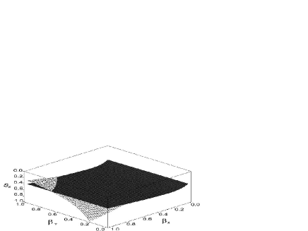
Figure 1: Bifurcations in a society of farmers, bandits and rulers. Stable dynasties occur in the topmost volume of the parameter space shown. If the availability of usable land $s_{\rm x}$ is increased the stability is lost as a Hopf bifurcation (dark surface) or a bifurcation of saddle-node type (light surface) is crossed. The Hopf bifurcation gives rise to oscillatory behavior that is known as the dynastic cycle. The fraction of farmer’s losses that occur because of crime $\beta_{\rm x}$ and the fraction of the bandits that get eventually caught $\beta_{\rm y}$ have only a weak effect on the stability of the dynasty.

In the figure the steady state under consideration is stable in the top-most volume of the parameter space. The stability of the steady state is lost in a Hopf bifurcation or in a bifurcation of saddle-node type. Since these bifurcations are of codimension one, the corresponding bifurcation points form hyper-surfaces in the parameter space. For the model under consideration the Hopf bifurcation surface is of particular interest. As this bifurcation surface is crossed the steady state becomes unstable while a limit cycle emerges. This gives rise to the dynastic cycle that is observed in simulations. The fact that the bifurcation surface lies almost perpendicular to the direction of $s_{\rm x}$ indicates that this parameter is of greater importance for the stability of the system than $\beta_{\rm x}$ or $\beta_{\rm y}$. Although such insights should be confirmed in a more careful mathematical investigation, they illustrate that bifurcation analysis of generalized models can be used to identify important parameters in a system.

The scale and exponent parameters which we have defined above capture only the local behavior of the generalized model. The bifurcation analysis which we can perform is therefore limited to the investigation of local bifurcations. Nevertheless, this analysis enables us to draw certain conclusions on the global dynamics of the generalized model. For example in Fig. 1 there is a line in which the Hopf bifurcation surface intersects the bifurcation surface of saddle-node type. The points on such a line are codimension-2 Gavrilov-Guckenheimer bifurcation points. The existence of these points implies that a region of complex (chaotic or quasiperiodic) dynamics exists generically in the model Kuznetsov (1995). In fact, it is shown in Feichtinger et al. (1974) that chaotic dynamics appear in a specific version of the generalized model considered here.

In summary we can say that the investigation of generalized models allows us to generalize insights from specific models. In particular, generalized models can be used to investigate the local dynamics (e.g. emergence of dynastic cycle from a Hopf bifurcation), to identify important parameters (e.g. availability of land $s_{\rm x}$) and to draw certain conclusions on the global dynamics (e.g. the existence of complex dynamics).

III A generalized model of coupled lasers

In the previous section we have shown that the local bifurcations of generalized models can be computed efficiently if the model is normalized in a certain way. This approach can be summarized in form of the following algorithm:

1. Formulation of a generalized model

2. Normalization

   • Define normalized variables and functions

   • Rewrite model in terms of the normalized quantities

   • Identify scale parameters

3. Computation of the Jacobian

   • Define exponent parameters

   • Interpret the exponent parameters

   • Compute the entries of the Jacobian matrix

4. Bifurcation analysis, …

We argue that essentially the same procedure can be applied to a large variety of different systems which can be described in the form of balance equations. In order to demonstrate this point we consider a system of coupled lasers. Although the scientific background is entirely different, it turns out that the laser model can be treated in the same way as the socio-economic model. For the analysis presented here the most striking difference between the physical and the socio-economic model is the amount of available information. In the socio-economic model all processes are difficult to quantify and are therefore candidates for generalization. By contrast, the underlying quantum mechanical foundations of laser physics are well understood. Many of the processes in the model can therefore be quantified with a high degree of certainty. Nevertheless, it can be useful to generalize certain processes which can be in principle quantified, but depend on many details of the specific system under consideration. In the following we show that the algorithm outlined above can be applied in such a partially generalized system.

III.1 Formulation of a model for coupled lasers

Models from laser physics are among the classical applications of the theory of dynamical systems Haken (1983); Mandel (1997); Lauterborn and Kurz (2005). In particular coupled lasers are known to exhibit interesting dynamics. The investigation presented here is inspired by the theoretical and experimental results reported in Fabiny et al. (1993); Jr. et al. (1997). In this work it is shown that the dynamics of two coupled single-mode lasers can be described by equations of the form

$$\begin{array}[]{r c l}\dot{A}_{1}&=&e_{1}A_{1}G_{1}+r_{1}G_{1}+\kappa\sqrt{A_{1}A_{2}}\cos(\delta)-L_{1}(A_{1})\\ \dot{A}_{2}&=&e_{2}A_{2}G_{2}+r_{2}G_{2}+\kappa\sqrt{A_{1}A_{2}}\cos(\delta)-L_{2}(A_{2})\\ \dot{G}_{1}&=&p_{1}-s_{1}G_{1}-r_{1}G_{1}-e_{1}A_{1}G_{1}\\ \dot{G}_{2}&=&p_{2}-s_{2}G_{2}-r_{2}G_{2}-e_{2}A_{2}G_{2}\\ \dot{\delta}&=&\frac{\kappa}{\tau_{c}}\left(\sqrt{\frac{A_{1}}{A_{2}}}+\sqrt{\frac{A_{2}}{A_{1}}}\right)\sin(\delta)-\delta_{0}\\ \end{array}$$ (20)

In order to discuss these equations, let us use the index $i=\{1,2\}$ to refer to laser 1 and 2 respectively. In the equations the intensity of laser $i$ is described by the variable $A_{i}$ while the gain of each laser is described by the variable $G_{i}$. The variable $\delta$ denotes the phase difference between laser $1$ and laser $2$.

The equations that governs the time evolution of $G_{i}$, the gain of laser $i$, contains four terms. The first term $p_{i}$ represents a constant pumping of the laser. The second term $s_{i}G_{i}$ describes the decrease of the gain because of spontaneous emission of photons which do not go into the laser mode. The term $r_{i}G_{i}$ represents spontaneous emission into the laser mode. The final term $e_{i}A_{i}G_{i}$ corresponds to stimulated emission. The quantities $p_{i}$, $s_{i}$, $r_{i}$ and $e_{i}$ that appear in these equations are assumed to be constants.

Spontaneous or stimulated emission of photons into the laser mode of laser $i$ increases the intensity $A_{i}$. This is described by the first two terms in the intensity equations. The third terms in these equations models the optical coupling of the lasers. The specific functional form of these terms as well as the equation that governs the evolution of the phase difference are results of Stratonovich calculus Fabiny et al. (1993). In these equations the constant $\kappa$ describes the strength of the coupling. The parameter $\tau_{c}$ is the cavity round trip time and $\delta_{0}$ is the difference of the phase velocity of the lasers without coupling.

The only general function that appears in the model equations is $L_{i}(A_{i})$. This function is used to describe the loss of laser intensity. Photons can be lost from the laser mode because of the absorbtion in the medium or because of escape from the resonator. Nonlinear optical effects like multi-photon absorbtion introduce nonlinearities in the intensity dependence of absorbtion inside the resonator Ciofini et al. (1993). Other nonlinear effects, like for instance temperature dependence or intensity dependence of the refractive index can effect the goodness of the resonator. As a consequence the losses of intensity can depend nonlinearly on the intensity. While all of these effects can be quantified for a specific laser medium, this would yield a complicated model that describes only one very specific type of laser. In many models studied in literature it is instead assumed that the losses depend linearly on the intensity of the laser.

III.2 Normalization of the physical model

Let us now normalize the generalized model formulated above. We start by assuming that there is at least one steady state. The dynamical variables in the steady state are denoted by ${A_{1}}^{*},{A_{2}}^{*},{G_{1}}^{*},{G_{2}}^{*}$ and $\delta^{*}$ respectively. Furthermore, we denote the values of the generalized functions in the steady state by ${L_{i}}^{*}$. As in the previous example we define the normalized state variables

$$\begin{array}[]{r c l}\displaystyle a_{i}&:=&\displaystyle\frac{A_{i}}{{A_{i}}^{*}}\\[5.0pt] \displaystyle g_{i}&:=&\displaystyle\frac{G_{i}}{{G_{i}}^{*}}\\ \end{array}$$ (21)

and the normalized function

$$l_{i}(a_{i}):=\displaystyle\frac{L_{i}({A_{i}}^{*}a_{i})}{{L_{i}}^{*}}\\$$ (22)

Normalization of the variable $\delta$ is not necessary. We could argue that $\delta$ is already an easily observable and interpretable variable, therefore the steady state value $\delta^{*}$ can be treated as a scale parameter. However in the following it will turn out that this reasoning is not necessary.

In the next step we rewrite the model in terms of the normalized variables. By substitution of Eq. (21) and Eq. (22) into Eq. (20) we obtain

$$\begin{array}[]{r c l}\displaystyle\dot{a}_{i}&=&\displaystyle\frac{e_{i}{A_{i}}^{*}{G_{i}}^{*}}{{A_{i}}^{*}}a_{i}g_{i}+\frac{r_{i}{G_{i}}^{*}}{{A_{i}}^{*}}g_{i}+\frac{\kappa\sqrt{{A_{1}}^{*}a_{1}{A_{2}}^{*}a_{2}}}{{A_{i}}^{*}}\cos(\delta)\\ &&\displaystyle-\frac{{L_{i}}^{*}}{{A_{i}}^{*}}l_{i}(a_{i})\\[5.0pt] \displaystyle\dot{g}_{i}&=&\displaystyle\frac{p_{i}}{{G_{i}}^{*}}-\frac{s_{i}{G_{i}}^{*}}{{G_{i}}^{*}}g_{i}-\frac{r_{i}{G_{i}}^{*}}{{G_{i}}^{*}}g_{i}-\frac{e_{i}{A_{i}}^{*}{G_{i}}^{*}}{{G_{i}}^{*}}a_{i}g_{i}\\[5.0pt] \displaystyle\dot{\delta}&=&\displaystyle\frac{\kappa}{\tau_{c}}\left(\sqrt{\frac{{A_{1}}^{*}a_{1}}{{A_{2}}^{*}a_{2}}}+\sqrt{\frac{{A_{2}}^{*}a_{2}}{{A_{1}}^{*}a_{1}}}\right)\sin(\delta)-\delta_{0}\\ \end{array}$$ (23)

where we have used the abbrieviating notation $L_{i}^{*}=L_{i}({A_{i}}^{*})$. In order to identify suitable scale parameters we consider the system in the steady state. This yields

$$\begin{array}[]{r c l}\displaystyle 0&=&\displaystyle e_{i}{G_{i}}^{*}+\frac{r_{i}{G_{i}}^{*}}{{A_{i}}^{*}}+\frac{\kappa\sqrt{{A_{1}}^{*}{A_{2}}^{*}}}{{A_{i}}^{*}}\cos(\delta^{*})-\frac{{L_{i}}^{*}}{{A_{i}}^{*}}\\[5.0pt] \displaystyle 0&=&\displaystyle\frac{p_{i}}{{G_{i}}^{*}}-s_{i}-r_{i}-e_{i}{A_{i}}^{*}\\[5.0pt] \displaystyle 0&=&\displaystyle\frac{\kappa}{\tau_{c}}\left(\sqrt{\frac{{A_{1}}^{*}}{{A_{2}}^{*}}}+\sqrt{\frac{{A_{2}}^{*}}{{A_{1}}^{*}}}\right)\sin(\delta^{*})-\delta_{0}\\ \end{array}$$ (24)

In the socio-economic model studied in the previous section we have seen that it is advantageous to group gain and loss terms together. In this way we obtain scale parameters that correspond to interpretable time scales. Grouping the terms in the laser model in this way we can identify the scale parameters

$$\begin{array}[]{r c l}\displaystyle\alpha_{i}&:=&\displaystyle e_{i}{G_{i}}^{*}+\frac{r_{i}{G_{i}}^{*}}{{A_{i}}^{*}}=-\frac{\kappa\sqrt{{A_{1}}^{*}{A_{2}}^{*}}}{{A_{i}}^{*}}\cos(\delta^{*})+\frac{{L_{i}}^{*}}{{A_{i}}^{*}}\\[5.0pt] \displaystyle\beta_{i}&:=&\displaystyle\frac{p_{i}}{{G_{i}}^{*}}=s_{i}+r_{i}+e_{i}{A_{i}}^{*}\end{array}$$ (25)

Note that we have treated the coupling term in the intensity equation as a loss term. This decision is motivated by the fact that frequency locking in experiments is generally observed to be anti-phase Jr. et al. (1997). In this case $\delta^{*}\approx\pi$ and $cos(\delta^{*})<0$. The analysis presented below will show that it is generally reasonable to consider the coupling term as a loss term. Our mathematical treatment of the system does not depend critically on the negativity of the coupling term. However, if the coupling term were positive it would be advisable to define the scale parameters in a different way for the sake of interpretation.

The way in which the scale parameters have been defined above allows us to identify the parameter $\alpha_{i}$ as the characteristic timescale of the intensity equation if $\pi/2\leq\delta^{*}\leq 3\pi/2$. In this case $\alpha_{i}$ is the per-capita (per-photon) loss rate of intensity of photons in the laser mode. In other words this $\alpha_{i}$ is the inverse of the typical lifetime of a photon in the laser mode of laser $i$. Likewise $\beta_{i}$ is the characteristic timescale of the gain equation or the inverse of the typical lifetime of atoms in the upper laser level.

In order to eliminate the constant factors from Eq. (23) we need to define additional scale variables which measure the contribution of the individual terms to the total gain and loss rates. We define the additional scale parameters

$$\begin{array}[]{r c l}\displaystyle\chi_{i}&:=&\displaystyle\frac{1}{\alpha_{i}}\frac{{L_{i}}^{*}}{{A_{i}}^{*}},\\[5.0pt] \displaystyle\sigma_{i}&:=&\displaystyle\frac{1}{\beta_{i}}(r_{i}+e_{i}{A_{i}}^{*}),\\[5.0pt] \displaystyle\gamma_{i}&:=&\displaystyle\frac{1}{\alpha_{i}}e_{1}{G_{i}}^{*}\end{array}$$ (26)

and the complementary parameters

$$\begin{array}[]{r c l}\displaystyle\tilde{\chi}_{i}&=&\displaystyle 1-\chi_{i}=-\frac{1}{\alpha_{i}}\frac{\kappa\sqrt{{A_{1}}^{*}{A_{2}}^{*}}}{{A_{i}}^{*}}cos(\delta^{*}),\\[5.0pt] \displaystyle\tilde{\sigma}_{i}&=&\displaystyle 1-\sigma_{i}=\frac{1}{\beta_{i}}s_{i},\\[5.0pt] \displaystyle\tilde{\gamma}_{i}&=&\displaystyle 1-\gamma_{i}=\frac{1}{\alpha_{i}}\frac{r_{i}{G_{i}}^{*}}{{A_{i}}^{*}}.\end{array}$$ (27)

Note that

$$\gamma_{i}=\displaystyle\frac{1}{\beta_{i}\sigma_{i}}e_{i}{A_{i}}^{*},\displaystyle\tilde{\gamma}_{i}=\displaystyle\frac{1}{\beta_{i}\sigma_{i}}r_{i}.$$ (28)

Finally we define

$$\rho:=\displaystyle\frac{A_{1}^{*}}{A_{2}^{*}}.$$ (29)

We can interpret the scale parameters as follows. The parameter $\chi_{i}$ denotes the fraction of the losses of intensity in laser $i$ that occur because of absorbtion or losses from the resonator. The complementary parameter $\tilde{\chi}_{i}$ is the fraction of the losses of laser $i$ that occur because of the coupling to the other laser. The parameter $\sigma_{i}$ describes the fraction of the total loss of gain of laser $i$ that corresponds to the production of photons in the laser mode. In a similar way the parameter $\gamma_{i}$ denotes the contribution of stimulated emission to this fraction. In other words, $\gamma_{i}$ denotes the fraction of photons in the laser mode of laser $i$ that were created by spontaneous emission.

The scale parameters allow us to write the model equations as

$$\begin{array}[]{r c l}\displaystyle\dot{a}_{i}&=&\displaystyle\alpha_{i}(\gamma_{i}a_{i}g_{i}+\tilde{\gamma}_{i}g_{i}-\tilde{\chi}_{i}\sqrt{a_{1}a_{2}}\frac{\cos(\delta)}{\cos(\delta^{*})}-\chi_{i}l_{i}(a_{i}))\\[5.0pt] \displaystyle\dot{g}_{i}&=&\displaystyle\beta_{i}(1-\tilde{\sigma}_{i}g_{i}-\sigma_{i}(\tilde{\gamma}_{i}g_{i}+\gamma_{i}a_{i}g_{i}))\\[5.0pt] \displaystyle\dot{\delta}&=&\displaystyle\frac{\kappa}{\tau_{c}}\left(\sqrt{\frac{\rho a_{1}}{a_{2}}}+\sqrt{\frac{a_{2}}{\rho a_{1}}}\right)\sin(\delta)-\delta_{0}\\ \end{array}$$ (30)

III.3 Computation of the Jacobian

Having completed the normalization we can now compute the Jacobian of the model. We start by defining the exponent parameter

$$\mu_{i}:=\displaystyle\left.\frac{\partial}{\partial a_{i}}l_{i}(a_{i})\right|_{a_{i}=1}\\$$ (31)

Using this parameter we can write the Jacobian in the steady state as

$${\rm\bf J}=\left(\begin{array}[]{c c c c c}\alpha_{1}&&&&\\ &\alpha_{2}&&&\\ &&\beta_{1}&&\\ &&&\beta_{2}&\\ &&&&\kappa/\tau_{c}\end{array}\right)\times\left(\begin{array}[]{c c c c c}\gamma_{1}-0.5\tilde{\chi}_{1}-\chi_{1}\mu_{1}&-0.5\tilde{\chi}_{1}&1&0&\tilde{\chi}_{1}\tan(\delta^{*})\\ -0.5\tilde{\chi}_{2}&\gamma_{2}-0.5\tilde{\chi}_{2}-\chi_{2}\mu_{2}&0&1&\tilde{\chi}_{2}\tan(\delta^{*})\\ -\sigma_{1}\gamma_{1}&0&-1&0&0\\ 0&-\sigma_{2}\gamma_{2}&0&-1&0\\ 0.5(\rho^{1/2}-\rho^{-1/2})\sin(\delta^{*})&0.5(\rho^{-1/2}-\rho^{1/2})\sin(\delta^{*})&0&0&(\rho^{1/2}+\rho^{-1/2})\cos(\delta^{*})\end{array}\right)$$ (32)

Let us assume that both lasers operate with same intensity in the steady state. This implies $\rho=1$. In this case all elements of the fifth row of the Jacobian vanish except for $J_{5,5}$. Therefore we can immediately identify the eigenvalue $\lambda_{5}=J_{5,5}=2\cos(\delta^{*})$. The existence of this eigenvalue proves that stable steady states are only possible for $\pi/2\leq\delta^{*}\leq 3\pi/2$. In this interval the stability of steady states is determined by the other four eigenvalues and therefore by the reduced Jacobian

$$\begin{array}[]{c}{\rm{\bf J}_{red}}=\left(\begin{array}[]{c c c c}\alpha_{1}&&&\\ &\alpha_{2}&&\\ &&\beta_{1}&\\ &&&\beta_{2}\end{array}\right)\times\\ \left(\begin{array}[]{c c c c}\gamma_{1}-0.5\tilde{\chi}_{1}-\chi_{1}\mu_{1}&-0.5\tilde{\chi}_{1}&1&0\\ -0.5\tilde{\chi}_{2}&\gamma_{2}-0.5\tilde{\chi}_{2}-\chi_{2}\mu_{2}&0&1\\ -\sigma_{1}\gamma_{1}&0&-1&0\\ 0&-\sigma_{2}\gamma_{2}&0&-1\end{array}\right)\end{array}$$ (33)

III.4 Computation of Bifurcations

Let us now study the bifurcations of the generalized laser model based on the reduced Jacobian. We simplify the reduced Jacobian further by assuming that the two lasers in the system are described by identical parameters ($\alpha_{1}=\alpha_{2}=:\alpha$, $\beta_{1}=\beta_{2}=:\beta$, $\gamma_{1}=\gamma_{2}=:\gamma$, $\chi_{1}=\chi_{2}=:\chi$, $\mu_{1}=\mu_{2}=:\mu$ and $\sigma_{1}=\sigma_{2}=:\sigma$). This assumption is valid for many coupled laser systems that are studied in experiments. Furthermore we set $\alpha=1$ by means of time normalization. As in the previous example we apply the method of resultants to compute the local bifurcations Gross and Feudel (2004). This reveals the bifurcation hypersurfaces of saddle-node type

$$\begin{array}[]{r c c c l}\displaystyle{\rm S1:}&\mu&=&\displaystyle\frac{\gamma(\sigma-1)}{\chi}&\mbox{for }\sigma<\frac{b}{\gamma}\\[5.0pt] \displaystyle{\rm S2:}&\mu&=&\displaystyle\frac{\gamma(\sigma-1)+1-\chi}{\chi}&\mbox{for }\sigma<\frac{b}{\gamma}\end{array}$$ (34)

and the Hopf bifurcation hyper-surfaces

$$\begin{array}[]{r c c c l}\displaystyle{\rm H1:}&\mu&=&\displaystyle\frac{\gamma-b}{\chi}&\mbox{for }\sigma<\frac{b}{\gamma}\\[5.0pt] \displaystyle{\rm H2:}&\mu&=&\displaystyle\frac{\gamma-b+\chi-1}{\chi}&\mbox{for }\sigma<\frac{b}{\gamma}\end{array}$$ (35)

These bifurcation surfaces are shown in Fig. 2. The steady state under consideration is stable in the top-most volume in the front of the left diagram. The right diagram shows the bifurcation surfaces from a different perspective so that the stable area is now in the back of the diagram. The stability is lost if one of the Hopf or saddle-node bifurcation surfaces is crossed. Note, that for $\sigma<b/\gamma$ both Hopf bifurcation surfaces are independent of $\sigma$. At $\sigma=b/\gamma$ both surfaces end simultaneously in Takens-Bogdanov bifurcation lines. The Takens-Bogdanov line of the Hopf bifurcation surface H1 is formed as it meets the bifurcation surface S1. At the same value of $\sigma$ the surface H2 ends in a Takens-Bogdanov bifurcation line as it meets S2. In addition to the Takens-Bogdanov lines there are two other codimension-2 bifurcation lines. A Gavrilov-Guckenheimer bifurcation is formed as H2 intersects S1. Finally, H1 and H2 meet in a double Hopf bifurcation line at $\chi=1$. All of these codimension-2 bifurcation lines meet in a single point at $\chi=1$, $\sigma=b/\gamma$. This point is a bifurcation point of codimension-4.

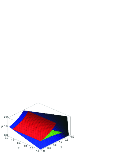
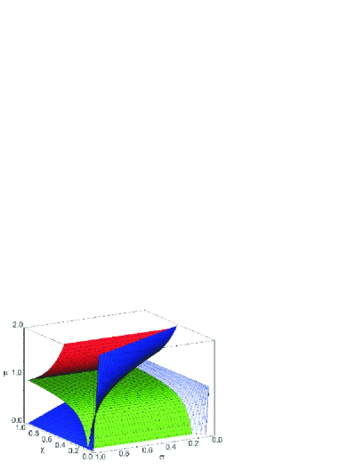
Figure 2: (Color) Two different perspectives on a three parameter bifurcation diagram of the coupled laser system. The steady state under consideration is stable in the volume that is located at high values of $\chi$ and $\mu$. The diagrams show the two saddle-node bifurcation surfaces S1 (dark blue) and S2 (light blue) and the two Hopf bifurcation surfafaces H1 (red) and H2 (green). At the intersection of these surfaces codimension-2 Takens-Bogdenov, Gavrilov-Guckenheimer and double Hopf bifurcations are formed. All codimension-2 lines meet in a codimension-4 quadruple point bifurcation. While the codimension-1 indicate the borders of the region of local stability, the bifurcations of higher codimension enable us to draw certain conclusions on the global dynamics.

As in the previous example the existence of bifurcations of higher codimension enables us to draw conclusions on the global dynamics of the system. The presence of Takens-Bogdanov bifurcations proves that a homoclinic bifurcation has to exist. This bifurcation corresponds to the formation of a homoclinic loop that connects one saddle to itself. Homoclinic loops are known to cause bursting behavior. In laser experiments such dynamics were observed in DeShazer et al. (2003); Jr. et al. (1997). Furthermore homoclinic bifurcations play an important role in the formation of Shilnikov chaos Glendinning (1994). In the previous section we have already mentioned that the Gavrilov-Guckenheimer bifurcation indicates the existence of a region of complex (at least quasiperiodic) dynamics. In a similar way the double Hopf bifurcation indicates the generic existence of a region in which chaos can be, at least transiently, observed Kuznetsov (1995).

The codimension-2 bifurcation lines do not only show that certain global dynamics do generically exist in the system. They also point to the parameter region where such dynamics are likely. For instance chaotic dynamics is likely close to the double Hopf bifurcation line. In this way the relatively simple computation of codimension-2 bifurcations can be used to locate interesting regions in parameter space. In these regions more time consuming techniques, like for instance the computation of Lyapunov exponents in specific models can then be applied.

IV A general food web model

In the previous sections we have applied the proposed approach to a generalized social model and to a partially generalized model of coupled lasers. In this section the same procedure is applied to a generalized model, which describes the dynamics of ecological food webs. The long term behavior and in particular the stability of food webs is investigated in a large number of theoretical and observational studies Steele and Henderson (1992); Ludwig et al. (1978); Blasius et al. (1999). In the following we compute the Jacobian of a generalized food web model. Since this model is more involved than the ones considered in the previous sections some additional difficulties arise. Nevertheless, the Jacobian can be constructed by following the algorithm outlined in Sec. III.

IV.1 Formulation of the ecological model

Let us consider a food web of $N$ ecological populations. We denote the size of these populations with dynamical variables $X_{1},\ldots,X_{N}$. For the sake of generality we do not distinguish between producer and consumer populations. Every population in the model can grow either by primary production (e.g. photosynthesis) or by consumption of prey (predation). The size of a given population can decrease because of predation by others or because of other causes of mortality (e.g. natural aging, diseases). We denote the primary production of population $n$ by the function $S_{n}(X_{n})$. The growth of population $n$ by predation on others is described by the functional response $F_{n}(X_{1},\ldots,X_{N})$. The loss inflicted by a higher predator $m$ is described by the function $L_{m,n}(X_{1},\ldots,X_{N})$. The mortality of species $n$ is denoted as $M_{n}(X_{n})$. Finally, we introduce the parameter $\eta$ which denotes the portion of consumed prey biomass that is converted into predator biomass. This yields the model

$$\begin{array}[]{r c l}\displaystyle\dot{X}_{n}&\displaystyle=&\displaystyle S_{n}(X_{n})+\eta_{n}F_{n}(X_{1},\ldots,X_{N})-M_{n}(X_{n})\\[5.0pt] \displaystyle\hfil&\displaystyle\hfil&\displaystyle-\sum_{m=1}^{N}L_{m,n}(X_{1},\ldots,X_{N})\end{array}$$ (36)

where $n=1,\ldots,N$.

In order to describe natural food webs in a realistic way we have to take an additional constraint into account. The loss rate of population $n$ because of predation by population $m$ is not unrelated to the growth rate $F_{m}$ of population $m$. In order to quantify this relationship we introduce the auxilliary variable $T_{m}(X_{1},\ldots,X_{N})$ which denotes the total amount of prey that is available to species $m$. It is reasonable to write $T_{m}(X_{1},\ldots,X_{N})$ as

$$T_{m}(X_{1},\ldots,X_{N})=\sum_{n=1}^{N}C_{m,n}(X_{n}),$$ (37)

where $C_{m,n}(X_{n})$ are auxilliary variables that describe the contribution of the population $n$ to the total amount of food available to population $m$. The value of $C_{m,n}(X_{n})$ depends not only on the density of population $n$ but also the preference of the predators for specific prey and on the success rate of attacks Gentleman et al. (2003).

We can now write the amount of prey consumed by population $m$ as

$$F_{m}(X_{1},\ldots,X_{N})=F_{m}(T_{m},X_{m}).$$ (38)

Since species $n$ contributes a fraction $C_{m,n}(X_{n})/T_{m}(X_{1},\ldots,X_{N})$ to the total amount of prey available to species $m$ it is reasonable to assume that it contributes the same fraction to the consumption rate. That means,

$$L_{m,n}(X_{1},\ldots,X_{N})=\frac{C_{m,n}(X_{n})}{T_{m}(X_{1},\ldots,X_{N})}F_{m}(T_{m},X_{m})$$ (39)

IV.2 Normalization of the ecological model

So far we have formulated a model of a $N$-species food web. In contrast to the models considered in the previous section we had to impose additional constaints in form of the algebraic equation Eq. (39). In the following we apply our normalization procedure to normalize these algebraic equations in addition to the ODEs.

Like in the previous sections we use asterics to indicate the values of functions and variables in the steady state. Using this notation, we define normalized state variables

$$x_{n}=\frac{X_{n}}{{X_{n}}^{*}}$$ (40)

normalized auxilliary variables

$$\begin{array}[]{r c l}t_{m}&:=&\displaystyle\frac{T_{m}({X_{1}}^{*}x_{1},\ldots,{X_{N}}^{*}x_{N})}{{T_{m}}^{*}},\\[5.0pt] c_{m,n}&:=&\displaystyle\frac{C_{m,n}({X_{n}}^{*}x_{n})}{{C_{m,n}}^{*}}\end{array}$$ (41)

and normalized functions

$$\begin{array}[]{r c l}s_{n}(x_{n})&:=&\displaystyle\frac{S_{n}({X_{n}}^{*}x_{n})}{{S_{n}}^{*}},\\[5.0pt] m_{n}(x_{n})&:=&\displaystyle\frac{M_{n}({X_{n}}^{*}x_{n})}{{M_{n}}^{*}},\\[5.0pt] f_{n}(x_{1},\ldots,x_{N})&:=&\displaystyle\frac{F_{n}({X_{1}}^{*}x_{1},\ldots,{X_{N}}^{*}x_{N})}{{F_{n}}^{*}},\\[5.0pt] l_{m,n}(x_{1},\ldots,x_{N})&:=&\displaystyle\frac{L_{m,n}({X_{1}}^{*}x_{1},\ldots,{X_{N}}^{*}x_{N})}{{L_{m,n}}^{*}}.\end{array}$$ (42)

As the second step of the normalization we rewrite the model in terms of the normalized quantities. We start by substituting the definitions Eqs. (40)-(42) into Eq. (36). This yields

$$\begin{array}[]{r c l}\dot{x}_{n}&=&\displaystyle\frac{{S_{n}}^{*}}{{X_{n}}^{*}}s_{n}(x_{n})+\frac{\eta_{n}{F_{n}}^{*}}{{X_{n}}^{*}}f_{n}(x_{1},\ldots,x_{N})\\[5.0pt] &&\displaystyle-\frac{M_{n}^{*}}{{X_{n}}^{*}}m_{n}(x_{n})-\sum_{m=1}^{N}\frac{{L_{m,n}}^{*}}{{X_{n}}^{*}}l_{m,n}(x_{1},\ldots,x_{N})\end{array}$$ (43)

In the next step we have to define suitable scale variables. We start with the time scales

$$\alpha_{n}:=\frac{{S_{n}}^{*}}{{X_{n}}^{*}}+\frac{\eta_{n}{F_{n}}^{*}}{{X_{n}}^{*}}=\frac{M_{n}^{*}}{{X_{n}}^{*}}+\sum_{m=1}^{N}\frac{{L_{m,n}}^{*}}{{X_{n}}^{*}}.$$ (44)

These scale parameters quantify the rate of biomass flow in the steady state. The relative contributions of the different processes to the biomass flow can be described by

$$\begin{array}[]{r c l}\rho_{n}&:=&\displaystyle\frac{1}{\alpha_{n}}\frac{\eta_{n}{F_{n}}^{*}}{{X_{n}}^{*}},\\[5.0pt] \tilde{\rho}_{n}&:=&\displaystyle 1-\rho_{n}=\frac{1}{\alpha_{n}}\frac{{S_{n}}^{*}}{{X_{n}}^{*}},\\[5.0pt] \sigma_{n}&:=&\displaystyle\frac{1}{\alpha_{n}}\sum_{m=1}^{N}\frac{{L_{m,n}}^{*}}{{X_{n}}^{*}},\\[5.0pt] \tilde{\sigma}_{n}&:=&\displaystyle 1-\sigma_{n}=\frac{1}{\alpha_{n}}\frac{M_{n}^{*}}{{X_{n}}^{*}},\\[5.0pt] \beta_{m,n}&:=&\displaystyle\frac{1}{\alpha_{n}\sigma_{n}}\frac{{L_{m,n}}^{*}}{{X_{n}}^{*}}.\end{array}$$ (45)

Before we discuss the interpretation of these parameters in more detail let us examine the algebraic equations in the model. We start with Eq. (39). In this case the substitution of the normalized quantities yields

$$\begin{array}[]{r c l}l_{m,n}(x_{1},\ldots,x_{N})&=&\displaystyle\frac{{C_{m,n}}^{*}{F_{m}}^{*}}{{T_{m}}^{*}{L_{m,n}^{*}}}\frac{c_{m,n}}{t_{m}}f_{m}(t_{m},x_{m})\\ &=&\displaystyle\frac{c_{m,n}}{t_{m}}f_{m}(t_{m},x_{m}),\end{array}$$ (46)

where we have used Eq. (39) in the second step.

The last equation which we have to consider is Eq. (37). In this case we obtain

$$t_{m}=\sum_{n=1}^{N}\frac{{C_{m,n}}^{*}}{{T_{m}}^{*}}c_{m,n}.$$ (47)

In contrast to Eq. (46) the constant factors do not cancel out in this equation. It is therefore useful to define the additional scale parameters

$$\chi_{m,n}=\frac{{C_{m,n}}^{*}}{{T_{m}}^{*}}.$$ (48)

We can now write the food web model as

$$\begin{array}[]{r c l}\dot{x}_{n}&=&\alpha_{n}(\tilde{\rho}_{n}s_{n}(x_{n})+\rho_{n}f_{n}(t_{n},x_{n})-\tilde{\sigma_{n}}m_{n}(x_{n})\\ &&-\sigma_{n}\sum_{m=1}^{N}\beta_{m,n}l_{m,n}(x_{1},\ldots,x_{N}))\end{array}$$ (49)

for $n=1\ldots N$ and

$$l_{m,n}(x_{1},\ldots,x_{N})=\frac{c_{m,n}}{t_{m}}f_{m}(t_{m},x_{m}),$$ (50)

$$t_{m}=\sum_{n=1}^{N}\chi_{m,n}c_{m,n}.$$ (51)

As a result of the normalization we have identified a set of scale parameters. Let us now discuss these parameters in more detail.

Based on our experience from the previous section we can identify the parameters $\alpha_{1},\ldots,\alpha_{N}$ immediately as the characteristic timescales of the system. The parameter $\alpha_{n}$ denotes the per-capita birth and death rate of population $n$ in the steady state. In other words, $\alpha_{n}$ is the inverse of the typical lifetime of individuals from population $n$.

The parameter $\rho_{n}$ is defined as the per-capita biomass gain of population $n$ divided by the total per-capita growth rate $\alpha_{n}$. In other words, this parameter describes what fraction of the growth rate of population $n$ is gained by predation. The complementary parameter $\tilde{\rho}_{n}$ denotes the fraction of the growth that originates from primary production. If population $n$ consists of primary producers the corresponding parameter values are $\rho_{n}=0,\tilde{\rho}_{n}=1$. A population of consumers has $\rho_{n}=1,\tilde{\rho}_{n}=0$. Some organisms are known which are capable of primary production and predation, for these $\rho_{n}$ and $\tilde{\rho}_{n}$ can have fractional values between zero and one.

The parameters $\sigma_{n}$ and $\tilde{\sigma}_{n}$ are very similar to $\rho_{n}$ and $\tilde{\rho}_{n}$. While $\rho_{n}$ and $\tilde{\rho}_{n}$ describe the relativ importance of the growth terms, $\sigma_{n}$ and $\tilde{\sigma}_{n}$ denote the relative importance of loss terms. The parameter $\sigma_{n}$ is defined as the fraction of the total loss rate of population $n$ that occurs because of predation by explicitly modelled predators. The fraction of losses that is caused by all other sources of mortality (e.g. natural mortality, diseases, predation by predators that are not explicitly modeled) is given by $\tilde{\sigma}_{n}$. We can therefore say, that the value of $\sigma_{n}$ indicates the predation pressure on species $n$.

The parameter $\beta_{m,n}$ is defined as the per-capita loss rate of population $n$ because of predation by population $m$ divided by the total loss rate of population $n$ because of predation $\alpha_{n}\sigma_{n}$. This means that $\beta_{m,n}$ denotes the relative weight of the contribution of species $m$ to predative loss rate of species $n$. If, for example, population $1$ is the only population that preys upon population $2$ then the corresponding parameter is $\beta_{1,2}=1$. However, if population $1$ causes only 50% of the losses while the other half is caused by predation by cannibalistic predation of population $2$ upon itself then we find $\beta_{1,2}=0.5$, $\beta_{2,2}=0.5$.

Finally, the parameter $\chi_{m,n}$ measures the relative contribution of population $n$ to the total amount of food that is available to species $m$. Note that, $\chi_{n,m}\neq\beta_{n,m}$. For example predation by species $1$ may only contribute, say $1/10$th of the total predative loss of species $2$. But, at the same time species $1$ may be the only species which is consumed by species $2$. In this situation we have $\beta_{1,2}=0.1$ but $\chi_{1,2}=1$.

IV.3 Computation of the Jacobian

Like in the previous examples we start the computation of the Jacobian by defining a set of exponent parameters that describe the nonlinearity of the ecological processes in the steady state

$$\begin{array}[]{r c l}\phi_{n}&:=&\left.\frac{\partial}{\partial x_{n}}s_{n}(x_{n})\right|_{{\rm\bf x}={\rm\bf x^{*}}},\\[5.0pt] \mu_{n}&:=&\left.\frac{\partial}{\partial x_{n}}m_{n}(x_{n})\right|_{{\rm\bf x}={\rm\bf x^{*}}},\\[5.0pt] \lambda_{m,n}&:=&\left.\frac{\partial}{\partial x_{n}}c_{m,n}(x_{n})\right|_{{\rm\bf x}={\rm\bf x^{*}}},\\[5.0pt] \gamma_{n}&:=&\left.\frac{\partial}{\partial t_{n}}f_{n}(t_{n},x_{n})\right|_{{\rm\bf x}={\rm\bf x^{*}}},\\[5.0pt] \psi_{n}&:=&\left.\frac{\partial}{\partial x_{n}}f_{n}({t_{n}}^{*},x_{n})\right|_{{\rm\bf x}={\rm\bf x^{*}}}.\end{array}$$ (52)

To a large extend these definitions follow the same scheme that we have applied in the previous sections. Note however that ${t_{n}}^{*}$ appears in the definition of $\psi_{n}$. In order to understand the reason for this definition we have to be aware of the fact that cannibalism can occur. Consequently, the amount of food $t_{n}$ that is available to the predator $x_{n}$ can depend on $x_{n}$ itself. The definition given above ensures that $\psi_{n}$ denotes only the nonlinearity of the predator-dependence of the response function.

The derivation of the Jacobian for the general food web model is analogous to the previous examples. For this reason the calculation is presented in appendix A. As a result we find that the non-diagonal elements of the Jacobian can be written as

$$\begin{array}[]{r c l}J_{n,i}&=&\alpha_{n}(\rho_{n}\gamma_{n}\chi_{n,i}\lambda_{n,i}-\sigma_{n}(\beta_{i,n}\psi_{i}\\ &&+\sum_{m=1}^{N}\beta_{m,n}\lambda_{m,i}(\gamma_{m}-1)\chi_{m,i}))\end{array}$$ (53)

and the diagonal elements as

$$\begin{array}[]{r c l}J_{i,i}&=&\alpha_{i}(\tilde{\rho}_{i}\phi_{i}+\rho_{i}(\gamma_{i}\chi_{i,i}\lambda_{i,i}+\psi_{i})\\ &&-\tilde{\sigma}_{i}\mu_{i}-\sigma_{i}(\beta_{i,i}\psi_{i}+\\ &&+\sum_{m=1}^{N}\beta_{m,i}\lambda_{m,i}((\gamma_{m}-1)\chi_{m,i}+1)))\end{array}$$ (54)

The parameter $\phi_{n}$ that appears in these equations describes the nonlinearity of the primary production of species $n$. In an environment where nutrient are abundant and no other limiting factors exist, it is reasonable to assume that the primary production $S_{n}$ is proportional to the number of primary producers $X_{n}$. This corresponds to $\sigma_{n}=1$. On the other hand, if nutrients are scarce then the primary production is limited by the nutrient supply. In this case the primary production is a constant function of the number of primary producers and $\sigma_{n}=0$. In a realistic situation $\sigma_{n}$ has a value between $0$ and $1$. This value can be interpreted as an indicator of the nutrient availability in the system.

The parameter $\mu_{n}$ denotes the nonlinearity of the mortality rate of population $n$. For top predators this parameter is often called exponent of closure in the ecological literature. More generally speaking, we call $\mu_{n}$ exponent of mortality. In most food web and food chain models this parameter is assumed to be either one or two. However, it has been shown that fractional values between one and two may describe natural systems in a more realistic way. This is discussed in detail in Edwards and Bees (2001).

The parameter $\gamma_{n}$ denotes the nonlinearity of the predation rate of population $n$ with respect to the prey density. If the prey is abundant then the predation rate is not limited by prey availability and $\gamma_{n}=0$. However, in most natural systems prey is relatively scarce. In this case the value of $\gamma_{n}$ can depend on the feeding strategy of population $n$. In the limit of scarce prey the value of $\gamma_{n}$ approaches one for predators of Holling type II and up to two for predators of Holling type III. This is discussed in more detail in Gross et al. (2004).

The parameter $\psi_{n}$ describes the dependence of the predation rate of population $n$ on the population density of $n$ itself. In most models it is assumed that predators of the same species feed independently without direct interference. In this case the predation rate is a linear function of the predator density and $\psi_{n}=1$. However, intraspecific competition or social interactions can introduce nonlinearities in the predator dependence of the predation rate. If these effects are taken into account we find $0<\psi_{n}<1$. An extreme example are the so-called ratio dependent models Abrams and Ginzburg (2000). These models correspond to $\psi_{n}=1-\gamma_{n}$.

Finally, the parameter $\lambda_{m,n}$ describes the nonlinearity of the contribution of population $m$ to the diet of population $n$. In the simplest case we can assume that the predator does not distuinguish actively between different prey types. An example of such a predator is an aquatic filtration feeder. In this case the contribution of a suitable prey population $m$ is proportional to the size of the population $m$ and $\lambda_{m,n}=1$. However, other predators attack their prey individually. These predators may adapt their strategies to a specific prey population if they have sufficient practice. In this case the success rate of attacks as well as the enounter rate increase linearly with the density of the prey population. In effect that leads to a quadratic dependence and therefore $\lambda_{m,n}=2$. Another type of behavior is exhibited by predators that need to choose their prey actively in order to obtain all nutrients that are necessary for growth. As an extreme example we could imagine a predator that requires exactly the right composition of its diet. In this case we find $\lambda_{m,n}=0$ for all prey populations $m$ but the limiting one.

IV.4 Stability of generalized food webs

In Sec. II and Sec. III we have used bifurcation analysis to study the Jacobians of the normalized models. For the investigation of food webs this analysis is also possible. In fact, bifurcation analysis has been used in Gross and Feudel (2004); Gross et al. (2004, 2005) to study the dynamics of generalized food chains. The generalized food chains considered in these papers are particular examples of the more general class of food webs considered here. The bifurcation analysis of other examples of generalized food webs can reveal new ecological insights. For instance we can consider bifurcation diagrams that correspond to different food web geometries. In this way one can investigate which food webs are characterized by a high local stability. Furthermore we can investigate the impact of certain ecological mechanisms on the stability or use higher codimension bifurcations to draw conclusions on the existence of complex dynamics. However, from the methodological point of view, these investigations are to a large extent parallel to the previous examples. Let us therefore describe a different way in which the derived Jacobian can be applied.

In order to investigate the stability of ecological systems random matrix models are frequently considered May (1973). In this context the Jacobian of a food web is modeled by a random matrix. The eigenvalues of a large set of these randomly created matrices are then computed. In this way one can for instance obtain a relationship between the stability of a random food web and the connectivity (often measured in terms of the number of non-diagonal elements of the matrix). While these analyses have provided many interesting results it has often been argued that not all of the randomly created matrices are biologically reasonable Haydon (2000).

The Jacobian of a generalized food web of given size can be studied in a similar way. By choosing the scale and exponent parameters randomly from suitable distributions one can create a set of random but realistic Jacobians. These Jacobians can then be studied by the numerical computation of eigenvalues. The advantage of this approach is that random matrices with certain ecological properties can be created. In this way one can for instance investigate the impact of ecological effects like intraspecific competition or cannibalism on the stability of the system. Although these investigations are certainly promising they require a much more detailed analysis and are therefore beyond the scope of the current paper.

V Discussion

In this paper we propose an approach to the investigation of generalized models which can be formulated in form of balance equations. In these equations gain and loss terms determine the time evolution of the state variables of the system under consideration. The proposed normalization procedure enables the researcher to consider a system from an abstract point of view. This abstractness is caused by the way in which variables and functions are normalized. The normalization procedure separates the necessary information about the steady state (the scale parameters) from the information about the nonlinearities in the model (the exponent parameters). In this way it becomes possible to study the effect of the nonlinearities independently from the location of the steady state. Apart from enabling us to investigate generalized models, this separation of scale and exponent variables has other advantages. For instance the elements of the Jacobians that are derived in this way are generally relatively simple. More importantly, it is in almost all models possible to identify the parameters in such a way that they are easily interpretable in the context of the model. In many cases the general parameters are more directly accessible to measurements than the specific parameters that are normally used in modeling. In Gross et al. (2004) it has been shown that the identification of the general parameters can in itself provide new insights.

The basic idea behind the proposed approach is to consider the bifurcations as functions of a new set of parameters which only encode as much information as is needed to construct the Jacobian. In this way we avoid the computation of steady states, which is in many cases more complicated than the computation of bifurcations once the Jacobian is known. This enables us to compute the local bifurcation surfaces analytically (using computer algebra systems) as a function of the scale and exponent parameters. As a result one is able to investigate the role of the nonlinearities in the gain and loss terms independently from the magnitude of these terms. In other words, one can study, with a high degree of generality, which functional forms of the gain and loss terms yields which dynamical behavior. Thus, this approach provides a bridge between modeling and stability analysis in dynamical systems theory.

The focus of the bifurcation analysis is the computation of local codimension-1 bifurcation of the normalized steady state. But, as a byproduct of this analysis we obtain the local bifurcations of higher codimension, which can reveal many insights about the dynamics in the neighborhood of these bifurcations. For instance the presence of a codimension-2 double Hopf bifurcation is an indicator for chaotic dynamics. Although our analysis is purely local, it can therefore reveal insights on the global dynamics of the system. In particular it can indicate regions in parameter space where complex dynamics can be expected. This insight can be used to prove the generic existence of chaotic parameter regions in generalized models or to locate interesting regions for subsequent numerical investigation.

At present there are only few results on the implications of local bifurcations of codimension larger than two. However, the opinion has often been expressed that this line of mathematical research would benefit from more examples from physical applications Guckenheimer and Holmes (2002). The approach proposed here provides physicist with a tool for finding these examples. In return, new mathematical results on the implications of bifurcations of higher codimension can be applied directly to the investigation of generalized models of physical systems. In this way, the investigation of generalized models may lead to more efficient transport of mathematical discoveries into physical applications and back.

Our approach to the investigation of generalized models is purely determistic. Noise and stochastic environmental fluctuations can not be accomodated adequately in the models considered here. However, the aim of the proposed approach is not to predict the time evolution of a given system, but rather to gain a general understanding of the functioning of a class of models. For systems with a low or moderate level of noise, the investigation of deterministic generalized models can still be useful, since it is unlikely that the presense of noise alters the local bifurcation structure qualitatively in this case.

The abstract nature of the proposed analysis becomes apparent if one considers that we did not have to specify which steady state we consider. In a system in which multiple steady states exist the derived bifurcation diagram does therefore describe all of these steady states simulateously. This insight can for instance be used to prove general statements of the type: “There can not be a stable steady state with …”.

In this paper, the main tool for the investigation of the derived Jacobians was bifurcation analysis. However, we have already remarked in our final example that the Jacobians can also be used in other ways. In particular large systems may contain too many parameters to be analysed efficiently with bifurcation diagrams. For these systems our method can be used in the random-matrix-like context, which is described in Sec. IV. In this light, the proposed method can be seen as a link between the very general random matrix approach and specific models.

Finally, let us remark that the approach presented here is not restricted to systems of ordinary differential equations. The algorithm which we have outlined in Sec. III can be applied in the same way to compute the bifurcations of discrete time maps. Moreover, it can be used in certain systems of partial differential equations to compute local bifurcations of homogenous solutions including Turing bifurcations Baurmann et al. .

*

Appendix A Computation of the Jacobian of the general food web

In this appendix we present the explicit comptation of the Jacobian of the food web model. We start by considering

$$\begin{array}[]{c}\left.\frac{\partial}{\partial x_{i}}t_{m}(x_{1},\ldots,x_{N})\right|_{{\rm\bf x}={\rm\bf x^{*}}}\\ =\left.\frac{\partial}{\partial x_{i}}\sum_{n=1}^{N}\chi_{m,n}c_{m,n}(x_{n})\right|_{{\rm\bf x}={\rm\bf x^{*}}}.\end{array}$$ (55)

We write the derivative of the predation rate as

$$\begin{array}[]{r c l}\frac{\partial}{\partial x_{i}}f_{n}(t_{n},x_{n})&=&\left(\frac{\partial}{\partial t_{n}}f_{n}(t_{n},x_{n})\right)\left(\frac{\partial}{\partial x_{i}}t_{n}\right)\\ &&+\left(\frac{\partial}{\partial x_{n}}f_{n}({t_{n}}^{*},x_{n})\right)\left(\frac{\partial}{\partial x_{i}}x_{n}\right).\end{array}$$ (56)

This yields

$$\left.\frac{\partial}{\partial x_{i}}f_{n}(t_{n},x_{n})\right|_{{\rm\bf x}={\rm\bf x^{*}}}=\left\{\begin{array}[]{l l}\gamma_{n}\chi_{n,i}\lambda_{n,i}&\mbox{for }i\neq n\\ \gamma_{n}\chi_{n,i}\lambda_{n,i}+\psi_{i}&\mbox{for }i=n\\ \end{array}\right.$$ (57)

Using this result we compute

$$\begin{array}[]{r c l}\left.\frac{\partial}{\partial x_{i}}l_{m,n}(x_{1},\ldots,x_{N})\right|_{{\rm\bf x}={\rm\bf x^{*}}}&=&-\chi_{m,i}\lambda_{m,i}+\gamma_{m}\chi_{m,i}\lambda_{m,i}+Q_{1}\\ &=&(\gamma_{m}-1)\chi_{m,i}\lambda_{m,i}+Q_{1}.\end{array}$$ (58)

where

$$Q_{1}=\left\{\begin{array}[]{l l}0&\hskip 28.45274pt\mbox{for }n\neq i,m\neq i\\ \lambda_{m,i}&\hskip 28.45274pt\mbox{for }n=i,m\neq i\\ \psi_{i}&\hskip 28.45274pt\mbox{for }n\neq i,m=i\\ \lambda_{m,i}+\psi_{i}&\hskip 28.45274pt\mbox{for }n=i,m=i\end{array}\right.$$ (59)

Let us now compute the derivatives of the sum in Eq. (49). We obtain

$$\begin{array}[]{c}\left.\frac{\partial}{\partial x_{i}}\sum_{m=1}^{N}\beta_{m,n}l_{m,n}(x_{1},\ldots,x_{N}))\right|_{{\rm\bf x}={\rm\bf x^{*}}}\\ =\beta_{i,n}\psi_{i}+\sum_{m=1}^{N}\beta_{m,n}\lambda_{m,i}((\gamma_{m}-1)\chi_{m,i}+Q_{2}).\end{array}$$ (60)

where

$$Q_{2}=\left\{\begin{array}[]{l l}1&\hskip 28.45274pt\mbox{for }i=n\\ 0&\hskip 28.45274pt\mbox{for }i\neq n\end{array}\right.$$ (61)

Using this result we can now write the non-diagonal elements as

$$\begin{array}[]{r c l}J_{n,i}&=&\alpha_{n}(\rho_{n}\gamma_{n}\chi_{n,i}\lambda_{n,i}-\sigma_{n}(\beta_{i,n}\psi_{i}\\ &&+\sum_{m=1}^{N}\beta_{m,n}\lambda_{m,i}(\gamma_{m}-1)\chi_{m,i})\end{array}$$ (62)

and the diagonal elements as

$$\begin{array}[]{r c l}J_{i,i}&=&\alpha_{i}(\tilde{\rho}_{i}\phi_{i}+\rho_{i}(\gamma_{i}\chi_{i,i}\lambda_{i,i}+\psi_{i})\\ &&-\tilde{\sigma}_{i}\mu_{i}-\sigma_{i}(\beta_{i,i}\psi_{i}\\ &&+\sum_{m=1}^{N}\beta_{m,i}\lambda_{m,i}((\gamma_{m}-1)\chi_{m,i}+1)))\end{array}$$ (63)

References

- Holling (1959) C. S. Holling, The Canadian Entomologist 91, 385 (1959).
- Gross et al. (2004) T. Gross, W. Ebenhöh, and U. Feudel, Journal of theoretical biology 227, 349 (2004).
- Fussmann and Blasius (2005) G. Fussmann and B. Blasius, Biology Letters 1, 9 (2005).
- Gross et al. (2005) T. Gross, W. Ebenhöh, and U. Feudel, Oikos 109, 135 (2005).
- Usher (1989) D. Usher, Am. Econ. Rev. 79, 1031 (1989).
- Feichtinger et al. (1974) G. Feichtinger, C. V. Forst, and C. Piccardi, Chaos, Solitons & Fractals 7, 257 (1996).
- Guckenheimer and Holmes (2002) J. Guckenheimer and P. Holmes, Nonlinear oscillations, dynamical systems, and bifurcations of vector fields (Springer, Berlin, 2002), 7th ed.
- Gross (2004) T. Gross, Population dynamics: General results from local analysis (Der Andere Verlag, Tönning, 2004).
- Kuznetsov (1995) Y. A. Kuznetsov, Elements of Applied Bifurcation Theory (Springer, Berlin, 1995).
- Gross and Feudel (2004) T. Gross and U. Feudel, Physica D 195, 292 (2004).
- Haken (1983) H. Haken, Synergetics: An Introduction (Springer Verlag, Berlin, 1983).
- Mandel (1997) P. Mandel, Theoretical problems in cavity nonlinear optics (Cambridge University Press, Cambridge, 1997).
- Lauterborn and Kurz (2005) W. Lauterborn and T. Kurz, Coherent Optics (Springer Verlag, Berlin, 2005).
- Fabiny et al. (1993) L. Fabiny, P. Colet, R. Roy, and D. Lenstra, Physical Review A47, 4287 (1993).
- Jr. et al. (1997) K. S. Thornburg, M. Möller, R. Roy, T. Carr, R.-D. Li, and T. Erneux, Physical Review E55, 3865 (1997).
- Ciofini et al. (1993) M. Ciofini, A. Politi, and R. Meucci, Physical Review A 48, 605 (1993).
- DeShazer et al. (2003) D. J. DeShazer, J. Garcia-Ojalvo, and R. Roy, Physical Review E 67, 036602 (2003).
- Glendinning (1994) P. Glendinning, Stability, Instability and Chaos: an introduction to the theory of nonlinear differential equations (Cambridge University Press, Cambridge, 1994).
- Steele and Henderson (1992) J. H. Steele and E. W. Henderson, J. Plankton Research 14, 157 (1992).
- Ludwig et al. (1978) D. Ludwig, D. D. Jones, and C. S. Holling, Journal of animal ecology 47, 315 (1978).
- Blasius et al. (1999) B. Blasius, A. Huppert, and L. Stone, Nature 399, 354 (1999).
- Gentleman et al. (2003) W. Gentleman, A. Leising, B. Frost, S. Storm, and J. Murray, Deep Sea Research II 50, 2847 (2003).
- Edwards and Bees (2001) A. M. Edwards and M. A. Bees, Chaos, Solitons and Fractals 12, 289 (2001).
- Abrams and Ginzburg (2000) P. A. Abrams and L. R. Ginzburg, Trends in Ecology and Evolution 15, 337 (2000).
- May (1973) R. M. May, Stability and Complexity in model ecosystems (Princeton University Press, Princeton, 1973).
- Haydon (2000) D. Haydon, Ecology 81, 2631 (2000).
- (27) M. Baurmann, T. Gross, and U. Feudel, submitted to Journal of Theoretical Biology.