Approximating multi-dimensional Hamiltonian flows by billiards.

Abstract

Consider a family of smooth potentials $V_{\epsilon}$, which, in the limit $\epsilon\rightarrow 0$, become a singular hard-wall potential of a multi-dimensional billiard. We define auxiliary billiard domains that asymptote, as $\epsilon\rightarrow 0$ to the original billiard, and provide asymptotic expansion of the smooth Hamiltonian solution in terms of these billiard approximations. The asymptotic expansion includes error estimates in the $C^{r}$ norm and an iteration scheme for improving this approximation. Applying this theory to smooth potentials which limit to the multi-dimensional close to ellipsoidal billiards, we predict when the separatrix splitting persists for various types of potentials.

1 Introduction

Imagine a point particle travelling freely (without friction) on a table, undergoing elastic collisions with the edges of the table. The table is just a bounded region of the plane. This model resembles a game of billiards, but it looks much simpler - we have only one ball, which is a dimensionless point particle. There is no friction and the table has no pockets. The shape of the table determines the nature of the motion (see [20] and references therein) - it can be ordered (integrable, e.g. in ellipsoidal tables), ergodic (e.g. in generic polygons), strongly mixing (in dispersing-Sinai tables or focusing-Bunimovich tables), or of a mixed nature for a general geometry with both concave and convex boundary components. A mechanical realization of this model in higher dimensions appears when one considers the motion of $N$ rigid $d$-dimensional balls in a $d$-dimensional box ($d=2$ or $3$): it corresponds to a billiard problem in a complicated $n$ dimensional domain, where $n=2N\times d$ ([29, 10]).

Usually, in the physics context, this billiard description is used to model a more complicated flow by which a particle is moving approximately inertially, and then is reflected by a steep potential. The reduction to the billiard problem simplifies the analysis tremendously, often allowing to describe completely the dynamics in a given geometry. Numerous applications of this idea appear in the physics literature; It works as idealized model for the motion of charged particles in a steep potential, a model which is often used to examine the relation between classical and quantized systems (see [17, 32] and references therein); This approximation was utilized to describe the dynamics of the motion of cold atoms in dark optical traps (see [18] and reference therein); This model has been suggested as a first step for substantiating the basic assumption of statistical mechanics – the ergodic hypothesis of Boltzmann ([21],[29],[30],[31],[33]). The opposite point of view may be taken when one is interested in studying numerically the hard wall system in a complicated geometry (e.g. apply ideas of [24] to [25]) - then designing the ”correct” limiting smooth Hamiltonian may simplify the complexity of the programming.

For two-dimensional finite-range axis-symmetric potentials [29, 22, 23, 1, 19, 15, 13, 2], it was shown that a modified billiard map may be defined, and several works have utilized this modified map to prove ergodicity of some configurations [29, 22, 23, 15, 2], or to prove that other configurations may possess stability islands [1, 13]. The general problem of studying the limiting process of making a steep two-dimensional potential steeper up to the hard-wall limit can be approached in a variety of ways. In [24] approach based on generalized functions was proposed. In [35] we developed a different paradigm for studying this problem. We first formulated a set of conditions on general smooth steep potentials in two-dimensional domains ($C^{r}$ smooth, not necessarily of finite range, nor axis-symmetric) which are sufficient for proving that regular reflections of the billiard flow and of the smooth flow are close in the $C^{r}$ topology. This statement, which may appear first as a mathematical exercise, is quite powerful. It allows to prove immediately the persistence of various kinds of billiard orbits in the smooth flows (see [35] and Theorem 5 in Section 3.4) and to investigate the behavior near singular orbits (e.g. orbits which are tangent to the boundary) by combining several Poincare maps, see for example [27, 36, 9]. The first part of this paper (see Theorems 1-2) is a generalization of this result to the multi-dimensional case.

Thus, it appears that the Physicists approach, of approximating the smooth flow by a billiard has some mathematical justification. How good is this approximation? Can this approach be used to obtain an asymptotic expansion to the smooth solutions? The second part of this paper answers these questions. We propose an approximation scheme, with a constructive twist - we show that the best zero-order approximation should be a billiard map in a slightly distorted domain. We provide the scaling of the width of the corresponding boundary layer with the steepness parameter and with the number of derivatives one insists on approximating. Furthermore, the next order correction is explicitly found, supplying a modified billiard map (reminiscent of the shifted billiard map of [29, 13]) which may be further studied. We believe this part is the most significant part of the paper as it supplies a constructive tool to study the difference between the smooth flow and the billiard flow.

Indeed, in the last part of this paper we demonstrate how these tools may be used to instantly extend novel results which were obtained for billiards to the steep potential setting; It is well known that the billiard map is integrable inside an ellipsoid [20]. Moreover, Birkhoff-Poritski conjecture claims that in 2 dimensions among all the convex smooth concave billiard tables only ellipses are integrable [34]. In [37] this conjecture was generalized to higher dimensions. Delshams et al ([11], [12] see references therein) studied the affect of small entire symmetric perturbations to the ellipsoid shape on the integrability. They proved that in some cases the separatrices of a simple periodic orbit split; Thus, they proved a local version of Birkhoff conjecture in the 2 dimensional setting, and provided several non-integrable models in the $n$ dimensional case. Here, we show that a simple combination of their results with ours, extends their result to the smooth case - namely it shows that the Hamiltonian flow, in a sufficiently steep potential which asymptotically vanishes in a shape which is a small perturbation of an ellipsoid, is chaotic. Furthermore, we quantify, for a given perturbation of the ellipsoidal shape, what “sufficiently steep” means for exponential, Gaussian and power-law potentials.

These results may give the impression that the smooth flow and the billiard flow are indeed very similar, and so a Scientist’s dream of greatly simplifying a complicated system is realized here. In the discussion we go back to this point - as usual dreams never materialize in full.

The paper is ordered as follows; In Section 2 we define and describe the billiard flow and billiard map. In Section 3 we study the smooth Hamiltonian flow; we first prove that if the potential satisfies some natural conditions the smooth regular reflections will limit smoothly to the billiard’s regular reflections (Theorems 1,2). Then, we define a natural Poincaré section on which a generalized billiard map may be defined for the smooth flow. Next, we derive the correction term to the zeroth order billiard approximation (Theorem 3) and calculate it for three model potentials (exponential, Gaussian and power-law). We end this section by stating its immediate implication - a persistence theorem for various types of trajectories (Theorem 5). In Section 4 we apply these results to the perturbed ellipsoidal billiard. We end the paper with a short summary and discussion. The appendices contain most of the proofs, whereas in the body of the paper we usually only indicate their main steps.

2 Billiards in $d$ dimensions

2.1 The Billiard Flow

Consider a billiard flow as the motion of a point mass in a compact domain $D\in\mathbb{R}^{d}$ or $\mathbb{T}^{d}$. Assume that the boundary $\partial D$ consists of a finite number of $C^{r+1}$ smooth ($r\geq 1$) $(d-1)$-dimensional submanifolds:

$$\partial D=\Gamma_{1}\cup\Gamma_{2}\cup...\cup\Gamma_{n},\;\;\;\;\;i=1\ldots n.$$ (1)

The boundaries of these submanifolds, when exist, form the corner set of $\partial D$:

$$\Gamma^{\ast}=\partial\Gamma_{1}\cup\partial\Gamma_{2}\cup...\cup\partial\Gamma_{n},\;\;\;\;\;i=1\ldots n.$$ (2)

The moving particle has a position $q\in D$ and a momentum vector $p\in\mathbb{R}^{d}$ which are functions of time. If $q\in int(D)$, then the particle moves freely with the constant velocity according to the rule:

$$\left\{\begin{array}[c]{l}\dot{q}=p\\ \overset{\cdot}{p}=0\end{array}\right..$$ (3)

Equation (3) is Hamiltonian with the Hamiltonian function (hereafter $p^{2}=\langle p,p\rangle$)

$$H(q,p)=\frac{p^{2}}{2}.$$ (4)

The particle moves at a constant speed and bounces of $\partial D$ according to the usual elastic reflection law : the angle of incidence is equal to the angle of reflection. This means that the outgoing vector $p_{out}$ is related to the incoming vector $p_{in}$ by

$$p_{out}=p_{in}-2\langle p_{in},n(q)\rangle n(q),$$ (5)

where $n(q)$ is the inward unit normal vector to the boundary $\partial D$ at the point $q$, see [10]. To use the reflection rule (5), we need the normal vector $n(q)$ to be defined, hence the rule cannot be applied at points $q\in\Gamma^{\ast}$, where such a vector fails to exist.

Definition 1.

The domain $D$ is called the configuration space of the billiard system.

The phase space of the system is $\mathcal{P}=D\times S^{d-1}$, where $S^{d-1}$ is a $(d-1)$-dimensional unit sphere (we set $H=\frac{1}{2}$) of velocity vectors. So the elements of $\mathcal{P}$ are

$$\rho\equiv(q,p).$$

Denote the time $t$ map of the billiard flow as

$$b_{t}:\rho_{0}\rightarrow\rho_{t}.$$ (6)

We do not consider reflections at the points of the corner set, so $\rho_{t}=b_{t}\rho_{0}$ implies here that the distance between any point on the trajectory connecting $q_{0}$ with $q_{t}$ and the set $\Gamma^{\ast}$ is bounded away from zero. A point $\rho\in\mathcal{P}$ is called an inner point if $q\notin\partial D$ and a collision point if $q\in\partial D\setminus\Gamma^{\ast}$. Obviously, if $\rho_{0}$ and $\rho_{t}=b_{t}\rho_{0}$ are inner points, then $\rho_{t}$ depends continuously on $\rho_{0}$ and $t$. If $\rho_{t}$ is a (non-tangent) collision point then the velocity vector undergoes a jump. Thus, in this case both $b_{t-0}$ and $b_{t+0}$ are defined. The map $R_{\circ}=b_{t+0}b_{t-0}^{-1}$ is the reflection law (5) (augmented by $q_{out}=q_{in}$).

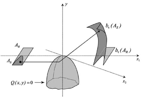
Figure 1: Singularity near a tangent trajectory. For better visualization we present a slanted hyperplane which is divided into 2 parts: $b_{\tau}$ has a square-root singularity on the boundary between $A_{R}$ and $A_{S}$.

If the piece of trajectory that connects $q_{0}$ with $q_{t}$ does not have tangencies with the boundary, then $\rho_{t}$ depends $C^{r}$-smoothly on $\rho_{0}$. It is well-known ([30],[35]) that the map $b_{t}$ loses smoothness at any point $q_{0}$ whose trajectory is tangent to the boundary at least once on the interval $(0,t)$. Clearly a tangency may occur only if the boundary is concave in the direction of motion at the point of tangency. Consider hereafter only non-degenerate tangencies, namely assume that the curvature in the direction of motion does not vanish.

Choose local coordinates $q=(x,y)$ in such a way that the origin corresponds to the collision point, the $y$-axis is normal to the boundary and looking inside the billiard region $D$, and the $x$-coordinates ($x\in\mathbb{R}^{d-1}$) correspond to the directions tangent to the boundary. If $Q(x,y)=0$ is the equation of the boundary in these coordinates, then $Q_{y}(0,0)\neq 0$ and $Q_{x}(0,0)=0$. We choose the convention that $Q_{y}(0,0)>0$. Obviously, the tangent trajectory is characterized by the condition $p_{y}=0$, where $(p_{x},p_{y})$ are the components of the momentum $p$. The vector $p_{x}=\dot{x}$ indicates the direction of motion of the tangent trajectory. It is easy to check that the tangency is non-degenerate if and only if

$$p_{x}^{T}Q_{xx}(0,0)p_{x}>0.$$ (7)

Notice that if the billiard’s boundary has saddle points (or if the billiard is semi-dispersing), then there always exist directions for which this non-degeneracy assumption fails. On the other hand, if the boundary is strictly concave, then all tangencies are non-degenerate.

Let $x=(x_{1},\dots,x_{d-1})$ with $x_{1}$ corresponding to the direction of motion (i.e. $p_{x}=(1,0,\dots,0)$). Then, the boundary surface near the point of non-degenerate tangency is described by the following equation:

$$y=-\alpha x_{1}^{2}+O(z^{2},x_{1}z),\qquad\alpha>0,$$

where we denote $z=(x_{2},\dots,x_{d-1})$. It is easy to see now that for a non-degenerate tangency, for a small $\tau$ the map $b_{\tau}$ of the line $\rho_{0}=(x_{0}=(-\tau/2,0,\dots,0),\;y_{0}\leq 0,\;p_{0x}=(1,0,\dots,0),\;p_{0y}=0)$ is given by

$$\rho_{\tau}=((\tau/2,0,\dots,0)+O(y_{0}),\ 2\tau\sqrt{-\alpha y_{0}}+O(y_{0}),\ (1,0,\dots,0)+O(y_{0}),\ 4\sqrt{-\alpha y_{0}}+O(y_{0})).$$

As we see, the billiard flow looses smoothness indeed (it has a square-root singularity in the limit $y\rightarrow-0$) near the tangent trajectory. See Figure 1.

2.2 The Billiard map

It is standard in dynamical system theory to reduce the study of flows to maps by constructing a cross-section. The latter is a hypersurface transverse to the flow. For the flow $b_{t}$, such a hypersurface in phase space $\mathcal{P}$ can be naturally constructed with the help of the boundary of $D$, i.e. the natural cross-section $S$ corresponds exactly to the collision points of the flow with the domain’s boundary:

$$S=\{\rho=(q,p)\in\mathcal{P}:q\in\partial D,\langle p,n(q)\rangle\geq 0\}.$$ (8)

This is a $(2d-2)$-dimensional submanifold in $\mathcal{P}$. Any trajectory of the flow $b_{t}$ crosses $S$ every time it reflects at $\partial D$. This defines the Poincaré map

$$B:S\rightarrow S\;\;\mathrm{such\;that}\;\;B\rho=b_{\tau_{\circ}(\rho)+0}\rho,$$ (9)

where

$$\tau_{\circ}(\rho)=\min\{t>0:b_{t+0}\rho\in S\}.$$

Definition 2.

The map $B$ is called the billiard map.

It is convenient to represent the billiard map as a composition of a free-flight and a reflection:

$$B=R_{\circ}\circ F_{\circ},$$

where the free-flight map is given by

$$F_{\circ}(q,p)=b_{\tau_{\circ}(\rho)-0}(q,p),$$ (10)

and the reflection law is given by

$$R_{\circ}(q,p)=(q,p-2\langle p,n(q)\rangle n(q)).$$

The billiard map $B$ is a $C^{r}-$diffeomorphism at all points $\rho\in S\setminus\Sigma$ such that $B\rho\in S\setminus\Sigma$, where $\Sigma$ is the singular set

$$\Sigma=\Sigma_{tangencies}\bigcup\Sigma_{corners}=\{(q,p)\in P:\langle p,n(q)\rangle=0\}\cup\{(q,p)\in P:q\in\Gamma^{\ast}\},$$ (11)

and $B$ is $C^{0}$ at the non-degenerate tangent trajectories.

3 Smooth Hamiltonian approximation

3.1 Setup and Conditions on Potential

Consider the family of Hamiltonian systems associated with:

$$H=\frac{p^{2}}{2}+V(q;\epsilon),$$ (12)

where the $C^{r+1}$-smooth potential $V(q;\epsilon)$ tends to zero inside a region $D$ as $\epsilon\rightarrow 0$, and it tends to infinity (or to a constant larger than the fixed considered energy level, say $H=\frac{1}{2}$) outside. Formally, the billiard flow in $D$ may be expressed as a limiting Hamiltonian system of the form:

$$H_{b}=\frac{p^{2}}{2}+V_{b}(q),$$ (13)

where

$$V_{b}(q)=\left\{\begin{array}[c]{ll}0&q\in D\\ +\infty&q\notin D\end{array}\right..$$ (14)

Let us formulate conditions under which this simplified billiard motion approximates the smooth Hamiltonian flow. In the two-dimensional case these conditions were introduced in [35].

Condition I. For any compact region $K\subset D$ the potential $V(q;\epsilon)$ diminishes along with all its derivatives as $\epsilon\rightarrow 0$:

$$\lim_{\epsilon\rightarrow 0}\|V(q;\epsilon)|_{q\in K}\|_{C^{r+1}}=0.$$ (15)

The growth of the potential to infinity across the boundary needs to be treated more carefully. We assume that $V$ is evaluated along the level sets of some finite function near the boundary. In other words, suppose, that in a neighborhood $\tilde{D}$ of $D\backslash\Gamma^{\ast}$ there exists a pattern function $Q(q;\epsilon):\tilde{D}\rightarrow\mathbb{R}^{1}$ which is $C^{r+1}$ with respect to $q$ and it depends continuously on $\epsilon$ (in the $C^{r+1}$-topology) at $\epsilon\geq 0$ (so it has, along with all derivatives, a proper limit as $\epsilon\rightarrow 0$). See Figure 2. Assume that away from $\Gamma^{\ast}$:

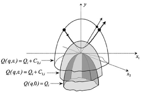
Figure 2: Level sets of a pattern function $Q(q;\epsilon)$. A bold line is a trajectory of the Hamiltonian flow near the boundary; a solid is a billiard trajectory.

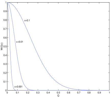
Figure 3: Gaussian potential given near the boundary by $W(Q;\epsilon)=e^{-\frac{Q^{2}}{\epsilon}}$ satisfies Conditions I-IV.

Condition IIa. The billiard boundary is composed of level surfaces of $Q(q;0)$:

$$Q(q;\epsilon=0)|_{q\in\Gamma_{i}}\equiv Q_{i}=\mathrm{constant}.$$ (16)

For each neighborhood of the boundary component $\Gamma_{i}$ (so $Q(q;\epsilon)$ is close to $Q_{i}$), let us define a barrier function $W_{i}(Q;\epsilon):\mathbb{R}^{1}\rightarrow\mathbb{R}^{1}$, which does not depend explicitly on $q$, and assume that:

Condition IIb. There exists a small neighborhood $N_{i}$ of the surface $\Gamma_{i}$ in which:

$$V(q;\epsilon)|_{q\in N_{i}}\equiv W_{i}(Q(q;\epsilon)-Q_{i};\epsilon),$$ (17)

and

Condition IIc.$\nabla V$ does not vanish in a finite neighborhood of the boundary surfaces, thus:

$$\nabla Q|_{q\in N_{i}}\neq 0$$ (18)

and

$$\frac{d}{dQ}W_{i}(Q-Q_{i};\epsilon)\neq 0.$$ (19)

Now, the rapid growth of the potential across the boundary may be described in terms of the barrier functions alone. Note that by (18), the pattern function $Q$ is monotonic across $\Gamma_{i}$, so either $Q>Q_{i}$ corresponds to the points near $\Gamma_{i}$ inside $D$ and $Q<Q_{i}$ corresponds to the outside, or vice versa.

Condition III. There exists a constant (may be infinite)$\mathcal{E}>0$ such that as $\epsilon\rightarrow+0$ the barrier function increases from zero to $\mathcal{E}$ across the boundary $\Gamma_{i}$:

$$\lim_{\epsilon\rightarrow+0}W(Q;\epsilon)=\left\{\begin{array}[c]{ll}0,&Q\text{~{}~{}inside~{}~{}}D\\ \mathcal{E},&Q\text{~{}~{}outside~{}~{}}D\end{array}\right..$$ (20)

By (19) $Q$ could be considered as a function of $W$ and $\epsilon$ near the boundary: $Q=Q_{i}+\mathcal{Q}_{~{}~{}i}(W;\epsilon)$. Condition IV states that for small $\epsilon$ a finite change in $W$ corresponds to a small change in $Q$:

Condition IV. As $\epsilon\rightarrow+0$, for any fixed $W_{1}$ and $W_{2}$ such that $0<W_{1}<W_{2}<\mathcal{E}$, for each boundary component $\Gamma_{i}$, the function $\mathcal{Q}_{~{}~{}i}(W;\epsilon)$ tends to zero uniformly on the interval $[W_{1},W_{2}]$ along with all its $(r+1)$ derivatives.

Figure 3 shows the geometric interpretation of the pattern function and a typical dependence of the barrier function on $Q$ and $\epsilon$.

Note that the use of the pattern and barrier functions essentially reduces the $d$-dimensional Hamiltonian dynamics to a $1$-dimensional one, which allows for a direct asymptotic integration of the smooth problem.

3.2 C⁰ and C^r - closeness Theorems

Theorem 1.

Let the potential $V(q;\epsilon)$ in (12) satisfy Conditions I-IV stated above. Let $h_{t}^{\epsilon}$ be the Hamiltonian flow defined by (12) on an energy surface $H=H^{\ast}<\mathcal{E}$, and $b_{t}$ be the billiard flow in $D$. Let $\rho_{0}$ and $\rho_{T}=b_{T}\rho_{0}$ be two inner phase points. Assume that on the time interval $[0,T]$ the billiard trajectory of $\rho_{0}$ has a finite number of collisions, and all of them are either regular reflections or non-degenerate tangencies. Then $h_{t}^{\epsilon}\rho_{\overset{\longrightarrow}{{}_{\epsilon\rightarrow 0}}}b_{t}\rho$, uniformly for all $\rho$ close to $\rho_{0}$ and all $t$ close to $T$.

Theorem 2.

In the conditions of Theorem 1, further assume that the billiard trajectory of $\rho_{0}$ has no tangencies to the boundary on the time interval $[0,T]$. Then $h_{t}^{\epsilon}~{}_{\overset{\longrightarrow}{{}_{\epsilon\rightarrow 0}}}b_{t}$ in the $C^{r}$-topology in a small neighborhood of $\rho_{0}$, and for all $t$ close to $T$.

The proof of the theorems is presented in the appendix and it follows closely the proof in [35]. Informally, the logic behind Conditions I-IV is as follows.

Condition I, obviously, implies that the particle moves with almost constant velocity (along a straight line) in the interior of $D$ until it reaches a thin layer near the boundary where $V$ runs from zero to large values (a smaller $\epsilon$ corresponds to a thinner boundary layer). Note that the boundary layer can not be fully penetrated by the particle. Indeed, as in all mechanical Hamiltonians, the energy level defines the region of allowed motion: for a fixed energy level $H=H^{\ast}<\mathcal{E}$, all trajectories stay in the region $V(q;\epsilon)\leq H^{\ast}$. It follows from Condition III that for any such $H^{\ast}$, the region of allowed motion approaches $D$ as $\epsilon\rightarrow 0$. Thus, by Condition III, if the particle enters the layer near a boundary surface (note that points from $\Gamma^{\ast}$ are not considered in this paper), it has, in principle, two possibilities. First, it may be reflected and then exits the boundary layer near the point it entered. The other possibility, which we want to avoid, is that the particle sticks to the boundary and travels along it far from the entrance point. Condition IV guarantees that if the reflection is regular, or in case of non-degenerate tangency, the travel distance along the boundary vanishes asymptotically with $\epsilon$. The case of degenerate tangencies, which are unavoidable in the higher dimensional case if the boundary has directional curvatures of opposite signs (namely saddle points), is not studied here. Once we know that the time spent by the particle near the boundary is small, we can see that Condition II guarantees that the reflection will be of the right character, namely the smooth reflection is $C^{0}$-close to that of the billiard. Indeed, Condition II implies that the reaction force is normal to the boundary, hence, as the time of collision is small and the position of the particle does not change much during this time, the direction of the force stays nearly constant during the collision. Thus, only the normal component of the momentum is changing sign while the tangent components are nearly preserved. Computations along these lines provide a proof of Theorem 1.

Proving Theorem 2, i.e. the $C^{r}$-closeness, makes a substantial use of Condition IV. Let us explain in more detail the difference between the $C^{0}$ and $C^{r}$ topologies in this context. Take the same initial condition $(q_{0},p_{0})$ for a billiard orbit and for an orbit of the Hamiltonian system (12) (the Hamiltonian orbit will be called the smooth orbit). Consider a time interval $t$ for which the billiard orbit collides with the boundary only once. In these notations $\varphi_{in}$ is the angle between $p_{0}$ (the momentum at the point $q_{0}$) and the normal to the boundary at the collision point, $\varphi_{out}$ is the angle between $p_{t}$ (the velocity vector at the point $q_{t}$) and the normal. Define the incidence and reflection angles ($\varphi_{in}(\epsilon)$ and $\varphi_{out}(\epsilon)$) for the smooth trajectory in the same way. Theorem 1 implies the correct reflection law for smooth trajectories:

$$\varphi_{in}(\epsilon)+\varphi_{out}(\epsilon)\approx 0$$ (21)

for sufficiently small $\epsilon$. However, $\varphi_{in}+\varphi_{out}$ is a function of the initial conditions, so a non-trivial question is when it is close to zero along with all its derivatives. In Theorem 2 we prove that Condition IV is sufficient for guaranteeing the correct reflection law in the $C^{r}$-topology in the case of non-tangent collision (near tangent trajectories the derivatives of the smooth flow cannot converge to those of the billiard because the billiard flow is singular there, see Figure 1).

Hereafter, we will fix the energy level of the Hamiltonian flow to $H^{\ast}=\frac{1}{2}$. Notice that the analysis may be applied to systems with steep potentials which do not depend explicitly on $\epsilon$ (or do not degenerate as $\epsilon\rightarrow 0$) in the limit of sufficiently high energy: the reduction to the setting (12) which we consider here may be achieved by a scaling of time.

3.3 Asymptotic for a regular reflection

It follows from the proof of Theorem 2 that the behavior of smooth trajectories close to billiard trajectories of regular reflections can be described by an analogue of the billiard map. More precisely, one can construct a cross-section $S_{\epsilon}$ in phase space of the Hamiltonian flow, close to the “natural” cross-section $S$ where the billiard map $B$ is defined; the trajectories of the Hamiltonian flow which are close to regular billiard trajectories define the Poincaré map on $S_{\epsilon}$, and this map is $C^{r}$-close to $B$. Let us explain this in more details.

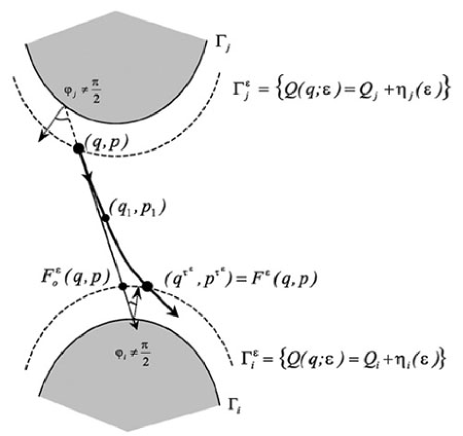
Figure 4: Free flight between boundaries $\Gamma_{i}^{\epsilon}$ and $\Gamma_{j}^{\epsilon}$. A smooth trajectory is marked by a bold line and an auxiliary billiard trajectory is marked by a solid line.

It is convenient to consider an auxiliary billiard in the modified domain $D^{\epsilon}$, defined as follows. For each boundary surface $\Gamma_{i}$, take any $\nu_{i}(\epsilon)\rightarrow+0$ such that the function (inverse barrier) $\mathcal{Q}_{~{}~{}i}(W;\epsilon)$ tends to zero along with all its derivatives, uniformly for $\frac{1}{2}\geq W\geq\nu_{i}$. We will use the notation

$$M_{i}^{(r)}(\nu;\epsilon)=\sup_{{\footnotesize\begin{array}[c]{c}\nu\leq W\leq\frac{1}{2}\\ 0\leq l\leq r+1\end{array}}}|\mathcal{Q}_{\;i}^{(l)}(W;\epsilon)|.$$ (22)

Condition IV implies that $M$ approaches zero as $\epsilon\rightarrow 0$ for any fixed $\nu>0$, hence the same holds true for any sufficiently slowly tending to zero $\nu(\epsilon)$, i.e. the required $\nu_{i}(\epsilon)$ exist. Let $\eta_{i}(\epsilon)=\mathcal{Q}_{~{}~{}i}(\nu_{i};\epsilon)$ and consider the billiard in the domain $D^{\epsilon}$ which is bounded by the surfaces $\Gamma_{i}^{\epsilon}:{Q(q;\epsilon)=Q_{i}+\eta_{i}(\epsilon)}$. See Figure 4. Recall that the boundaries $\Gamma_{i}$ of the original billiard table $D$ are level sets $Q(q;0)=Q_{i}$, and that $\eta_{i}(\epsilon)\rightarrow 0$ by construction, so the new billiard is close to the original one. In particular, for regular reflections, the billiard map $B^{\epsilon}$ of the auxiliary billiard tends to the original billiard map $B$ along with all its derivatives. It is established in the proof of Theorem 2 that for any choice of $\nu_{i}$’s tending to zero, the condition $q\in\partial D^{\epsilon}$ defines a cross-section in the phase space of the smooth Hamiltonian flow; Trajectories which are close to the billiard trajectories of regular reflection, i.e. those which intersect $\partial D^{\epsilon}$ at an angle bounded away from zero, define the map

$$F^{\epsilon}:(q\in\partial D^{\epsilon},p\;\;\mbox{ looking inwards }\;D^{\epsilon})\rightarrow(q\in\partial D^{\epsilon},p\;\;\mbox{ looking outwards }\;D^{\epsilon}),$$

namely

$$F^{\epsilon}(q,p)=h_{\tau^{\epsilon}}^{\epsilon}(q,p)$$ (23)

and this map is close to the free-flight map $F_{\circ}^{\epsilon}$ (see Section 2.2) of the billiard in $D^{\epsilon}$:

$$F_{\circ}^{\epsilon}(q,p)=b_{\tau_{\circ}^{\epsilon}-0}(q,p)$$ (24)

where $\tau^{\epsilon}(q,p)$ is the time the smooth Hamiltonian orbit of $(q,p)$ needs to reach $\partial D^{\epsilon}$, and $\tau_{\circ}^{\epsilon}(q,p)$ denotes the same for the billiard orbit. Note that we cannot claim the closeness of the time $\tau$ maps for the smooth Hamiltonian and billiard flows everywhere in $D^{\epsilon}$, still we claim that the maps (23) and (24) are close; we will return to this later.

Outside $D^{\epsilon}$, the overall effect of the motion of smooth orbits is close to that of a billiard reflection. Namely, as it is proved in Theorem 2, once $\nu_{i}$ is chosen such that $M_{i}^{(r)}(\nu_{i},\epsilon)\rightarrow 0$, the smooth trajectories which enter the region $W_{i}(Q;\epsilon)\geq\nu_{i}$ at a bounded away from zero angle to the boundary, spend in this region a small interval of time (denoted by $\tau_{c}^{\epsilon}(q_{in},p_{in})$) after which they return to the boundary $W_{i}(Q;\epsilon)=\nu_{i}$ (namely to $Q(q;\epsilon)=Q_{i}+\eta_{i}(\epsilon)$). Thus, these orbits define the map

$$R^{\epsilon}:(q_{in}\in\partial D^{\epsilon},p_{in}\;\;\mbox{ looking outwards }\;D^{\epsilon})\rightarrow(q_{out}\in\partial D^{\epsilon},p_{out}\;\;\mbox{ looking inwards }\;D^{\epsilon}).$$

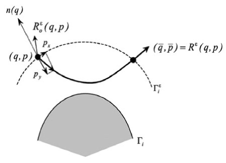
Figure 5: Reflection from the boundary $\Gamma_{i}$. A smooth trajectory is marked by a bold line. An auxiliary billiard trajectory only changes its direction according to the law (25).

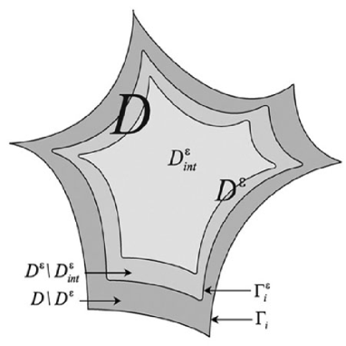
Figure 6: The partition of the domain $D$ into regions: $D^{\epsilon}_{int}\subset D^{\epsilon}$.

It follows from the proof of Theorem 2 that the map $R^{\epsilon}$ is close to the standard reflection law $R_{\circ}^{\epsilon}$ from the boundary $\partial D^{\epsilon}$:

$$R_{\circ}^{\epsilon}(q,p)=\left(q,p-2n(q)\left\langle n(q),p\right\rangle\right),$$ (25)

where $n(q)$ is the unit normal vector to the boundary $\partial D^{\epsilon}$ at the point $q$. See Figure 5. Note that the smooth reflection law $R^{\epsilon}$ corresponds to a non-zero (though small) collision time $\tau_{c}^{\epsilon}(q,p)$, unlike the billiard reflection $R_{\circ}^{\epsilon}$ which happens instantaneously. Summarizing, from the proof of Theorem 2 we extract that on the cross-section

$$S_{\epsilon}=\{\rho=(q,p):q\in\partial D^{\epsilon},\langle p,n(q)\rangle>0\}$$ (26)

the Poincaré map

$$\Phi^{\epsilon}=R^{\epsilon}\circ F^{\epsilon}$$ (27)

is defined for the smooth Hamiltonian flow (for regular orbits - orbits which intersect $\partial D^{\epsilon}$ at an angle bounded away from zero), and this map is $C^{r}$-close to the billiard map $B^{\epsilon}=R_{\circ}^{\epsilon}\circ F_{\circ}^{\epsilon}$. As the billiard map $B^{\epsilon}$ is close to the original billiard map $B$, we obtain the closeness of the Poincaré map $\Phi^{\epsilon}$ to $B$ as well. However, when developing asymptotic expansions for $\Phi^{\epsilon}$, it is convenient to use the map $B^{\epsilon}$ (rather than $B$) as the zeroth order approximation for $\Phi^{\epsilon}$. Then, the next term in the asymptotic may be explicitly found (see below) and the whole asymptotic expansion may be similarly developed.

We start with the estimates for the “free flight” segment of the motion, i.e. for the smooth Hamiltonian trajectories inside $D^{\epsilon}$. For every boundary surface $\Gamma_{i}$, choose some $\delta_{i}(\epsilon)\rightarrow 0$ such that the surfaces $Q(q;\epsilon)=Q_{i}+\delta_{i}(\epsilon)$ bound the region $D_{int}^{\epsilon}$ inside $D^{\epsilon}$ in which the potential $V$ tends to zero uniformly along with all its derivatives. See Figure 6. Let

$$m^{(r)}(\delta;\epsilon)=\sup_{{\footnotesize\begin{array}[c]{c}q\in D_{int}^{\epsilon}\\ 1\leq l\leq r+1\end{array}}}\|\partial^{l}V(q;\epsilon)\|.$$ (28)

According to Condition I, $m$ approaches zero as $\epsilon\rightarrow 0$ for any fixed $\delta$ of the appropriate signs, therefore the same holds true for any choice of sufficiently slowly tending to zero $\delta_{i}(\epsilon)$. As $m^{(r)}\rightarrow 0$, it follows that within $D_{int}^{\epsilon}$ the flow of the smooth Hamiltonian trajectories is $C^{r}$-close to the free flight, i.e. to the billiard flow. In other words, the time $\tau$ map $h_{\tau}^{\epsilon}(q,p)=(q_{\tau},p_{\tau})$ of the smooth flow in $D_{int}^{\epsilon}$ is $O_{{}_{C^{r}}}(m^{(r)})$-close to the time $\tau$ map of the billiard flow

$$b_{\tau}(q,p)=\begin{pmatrix}q+p\tau\\ p\end{pmatrix}.$$ (29)

Note that on the boundary of $D^{\epsilon}$ we have, by construction, $\mathcal{Q}_{\;i}^{\prime}(W;\epsilon)\rightarrow 0$, i.e. $W_{i}^{\prime}(Q;\epsilon)\rightarrow\infty$, while on the boundary of $D_{int}^{\epsilon}$ we have $W_{i}^{\prime}(Q;\epsilon)\rightarrow 0$. Thus, we have a boundary layer $D^{\epsilon}\backslash D_{int}^{\epsilon}$ of a non-zero width $\left|\delta_{i}(\epsilon)-\eta_{i}(\epsilon)\right|$ in which the gradient of the potential rapidly decreases. The speed with which the value of $Q(q(t);\epsilon)$ changes within this boundary layer is bounded away from zero (see the proof of Theorem 2), so the time the orbit needs to penetrate it is $O(\delta_{i})$. Within this boundary layer the time $\tau$ map $(q,p)\mapsto(q_{\tau},p_{\tau})$ of the smooth flow is not necessarily close to the time $\tau$ map of the billiard flow (29). However, it is shown in the proof of Theorem 2, that the maps from one surface $Q=const$ to any other such surface within the boundary layer are $C^{r}$-close for the two flows. This, obviously, implies the closeness of the maps $F^{\epsilon}$ and $F_{\circ}^{\epsilon}$ (because the corresponding cross-section is the surface of the kind $Q=const$ indeed).

In Appendix 7.2 we show that by an appropriate change of coordinates in each of the three regions we consider (inside $D_{int}^{\epsilon}$, in $D^{\epsilon}\backslash D_{int}^{\epsilon}$, and outside $D^{\epsilon}$), the equations of motion may be written as differential equations integrated over a finite interval with a right hand side which tends to zero in the $C^{r}$-topology as $\epsilon\rightarrow 0$. Thus, not only do we obtain error estimates for the zeroth order approximation, we also find a method for obtaining higher order corrections using Picard iterations; The asymptotic behavior of the right hand side of the equations leads to a contractivity constant which asymptotically vanishes and thus the Picard iteration scheme provides asymptotic for the solutions (each new iteration provides a better asymptotic). In this way we prove in appendix 7.3 the following

Lemma 1.

Let $q$ be an inner point of $D$, and $p$ be such that the first hit of the billiard orbit of $(q,p)$ with the boundary $\Gamma_{i}$ is non-tangent. Then, the orbit of the smooth flow hits the cross-section $\{q\in\Gamma_{i}^{\epsilon}\}=\{Q(q;\epsilon)=Q_{i}+\eta_{i}(\epsilon)\}$ at the point $(q_{\tau},p_{\tau})$ such that

$$\begin{array}[c]{ccc}q_{\tau}&=&q+p\tau+O_{{}_{C^{r}}}(m^{(r)}+\nu_{i})\\ &=&q+p\tau+\int_{0}^{\tau}\nabla V(q+ps;\epsilon)(s-\tau)ds+O_{{}_{C^{r-1}}}((m^{(r)}+\nu_{i})^{2}),\\ p_{\tau}&=&p+O_{{}_{C^{r}}}(m^{(r)}+\nu_{i})\\ &=&p-\int_{0}^{\tau}\nabla V(q+ps;\epsilon)ds+O_{{}_{C^{r-1}}}((m^{(r)}+\nu_{i})^{2}),\end{array}$$ (30)

where $\tau=\tau^{\epsilon}(q,p)$ denotes the travel time to the boundary of $D^{\epsilon}$ (so $Q(q_{\tau};\epsilon)=Q_{i}+\eta_{i}(\epsilon)$):

$$\begin{array}[c]{ccc}\tau^{\epsilon}(q,p)&=&\tau_{\circ}^{\epsilon}(q,p)+O_{{}_{C^{r}}}(m^{(r)}+\nu_{i})\\ &=&\tau_{\circ}^{\epsilon}(q,p)+\frac{\langle\nabla Q,\int_{0}^{\tau_{\circ}^{\epsilon}}\nabla V(q+ps;\epsilon)(\tau_{\circ}^{\epsilon}-s)ds\rangle}{\langle\nabla Q,p\rangle}+O_{{}_{C^{r-1}}}((m^{(r)}+\nu_{i})^{2}),\end{array}$$ (31)

where $\nabla Q$ is evaluated at the (auxiliary) billiard collision point $q+p\tau_{\circ}^{\epsilon}(p,q)$, and $\tau_{\circ}^{\epsilon}(p,q)$ is the time the billiard orbit of $(q,p)$ needs to reach $\Gamma_{i}^{\epsilon}$.

Now, let us estimate the free-flight map $F^{\epsilon}$ of the Hamiltonian flow. If $q\in\Gamma_{j}^{\epsilon}$ and $\langle p,n(q)\rangle$ is positive and bounded away from zero, and if the straight line issued from $q$ in the direction of $p$ first intersects $\partial D^{\epsilon}$ (say, the surface $\Gamma_{i}^{\epsilon}$) transversely as well (in our notations this can be expressed as the condition that $\langle p,n(q+p\tau^{\epsilon}_{\circ}(q,p))\rangle$ is negative and bounded away from zero), then the orbits of the Hamiltonian flow define the map $F^{\epsilon}$ from a small neighborhood of $(q,p)$ on the cross-section $\{q\in\Gamma_{j}^{\epsilon}\}$ in phase space into a small neighborhood of the point $(q+p\tau^{\epsilon}_{\circ}(q,p),p)$ on the cross-section $\{q\in\Gamma_{i}^{\epsilon}\}$. See Figure 4. Take an inner point $(q_{1},p_{1})$ on the smooth Hamiltonian trajectory of $(q,p)$. By construction (see (23)),

$$\tau^{\epsilon}(q,p)=\tau^{\epsilon}(q_{1},-p_{1})+\tau^{\epsilon}(q_{1},p_{1}),$$

$$(q,p)=h^{\epsilon}_{-\tau^{\epsilon}(q_{1},-p_{1})}(q_{1},p_{1})$$

and

$$F^{\epsilon}(q,p)=h^{\epsilon}_{\tau^{\epsilon}(q_{1},p_{1})}(q_{1},p_{1}).$$

As $q_{1}$ is bounded away from the billiard boundary, we can plug (30) and (31) in these relations, which gives us the following

Lemma 2.

Near the point $(q,p)$ under consideration, the free flight map $F^{\epsilon}:(q,p)\mapsto(q_{{}_{\tau^{\epsilon}}},p_{{}_{\tau^{\epsilon}}})$ for the smooth Hamiltonian flow is $O_{{}_{C^{r}}}(m^{(r)}+\nu_{i}+\nu_{j})$-close to the free flight map $F_{\circ}^{\epsilon}$ of the billiard in $D^{\epsilon}$ and is given by

$$\begin{array}[c]{l}q_{{}_{\tau^{\epsilon}}}=q+p\tau^{\epsilon}+\int_{0}^{\tau^{\epsilon}}\nabla V(q+ps;\epsilon)(s-\tau^{\epsilon})ds+O_{{}_{C^{r-1}}}((m^{(r)}+\nu_{i}+\nu_{j})^{2}),\\ p_{{}_{\tau^{\epsilon}}}=p-\int_{0}^{\tau^{\epsilon}}\nabla V(q+ps;\epsilon)ds+O_{{}_{C^{r-1}}}((m^{(r)}+\nu_{i}+\nu_{j})^{2}).\end{array}$$ (32)

The flight time $\tau^{\epsilon}(q,p)$ is $O_{{}_{C^{r}}}(m^{(r)}+\nu_{i}+\nu_{j})$-close $\tau_{\circ}^{\epsilon}(p,q)$ and is uniquely defined by the condition $Q(q_{\tau^{\epsilon}};\epsilon)=Q_{i}+\eta_{i}(\epsilon)$ (cf.(31)):

$$\tau^{\epsilon}(q,p)=\tau_{\circ}^{\epsilon}(q,p)+\frac{\langle\nabla Q,\int_{0}^{\tau_{\circ}^{\epsilon}}\nabla V(q+ps;\epsilon)(\tau_{\circ}^{\epsilon}-s)ds\rangle}{\langle\nabla Q,p\rangle}+O_{{}_{C^{r-1}}}((m^{(r)}+\nu_{i}+\nu_{j})^{2}),$$ (33)

where $\nabla Q$ is taken at the billiard collision point $q+p\tau_{\circ}^{\epsilon}(p,q)$ and $\tau_{\circ}^{\epsilon}(p,q)$ corresponds to the free flight travel time: $Q(q+p\tau_{\circ}^{\epsilon}(p,q);\epsilon)=Q_{i}+\eta_{i}(\epsilon).$

This could be written as

$$F^{\epsilon}=F^{\epsilon}_{\circ}+O_{{}_{C^{r}}}(m^{(r)}+\nu_{i}+\nu_{j})=F^{\epsilon}_{\circ}+F^{\epsilon}_{1}+O_{{}_{C^{r-1}}}((m^{(r)}+\nu_{i}+\nu_{j})^{2}),$$

where $F^{\epsilon}_{1}=O_{{}_{C^{r}}}(m^{(r)}+\nu_{i}+\nu_{j})$ and $F^{\epsilon}_{\circ}$ is defined by 24.

Note that the above estimates hold true for any choice of $\delta_{i}$’s such that $m^{(r)}\rightarrow 0$. Therefore, one may take $\delta_{i}$’s tending to zero as slow as needed in order to ensure as good estimates as possible for the error terms in (32),(33).

Next we estimate the reflection law $R^{\epsilon}$ for the smooth orbit. Consider a point $q\in\Gamma_{i}^{\epsilon}$ and let the momentum $p$ be directed outside $D^{\epsilon}$, at a bounded from zero angle with $\Gamma_{i}^{\epsilon}$. As we explained, the smooth trajectory of $(q,p)$ spends a small time $\tau_{c}^{\epsilon}(q,p)$ outside $D^{\epsilon}$ and then returns to $\Gamma_{i}^{\epsilon}$ with the momentum directed strictly inside $D^{\epsilon}$. Let $p_{y}$ and $p_{x}$ denote the components of momentum, respectively, normal and tangential to the boundary $\Gamma_{i}^{\epsilon}$ at the point $q$:

$$p_{y}=\langle n(q),p\rangle,\qquad p_{x}=p-p_{y}n(q).$$ (34)

We assume that the unit normal $n(q)$ is oriented inside $D^{\epsilon}$, so $p_{y}<0$ at the initial point. Denote by $Q_{y}(q;\epsilon)$ the derivative of $Q$ in the direction of $n(q)$:

$$Q_{y}(q;\epsilon):=\langle\nabla Q(q;\epsilon),n(q)\rangle,$$

let $K(q;\epsilon)$ denote the derivative of $n(q)$ in the directions tangent to $\Gamma_{i}^{\epsilon}$, and let $l(q;\epsilon)$ denote the derivative of $n(q)$ in the direction of $n(q)$. Obviously, $Q_{y}$ is a scalar, $K$ is a matrix and $l$ is a vector tangent to $\Gamma_{i}^{\epsilon}$ at the point $q$. Note that $Q_{y}\neq 0$ by virtue of Condition IIc. Define the integrals:

$$\begin{array}[c]{l}I_{1}=I_{1}(q,p)=2\int_{0}^{-p_{y}}\mathcal{Q}_{\;i}^{\prime}(\frac{1-p_{x}^{2}-s^{2}}{2};\epsilon)ds\\ I_{2}=I_{2}(q,p)=2\int_{0}^{-p_{y}}\mathcal{Q}_{\;i}^{\prime}(\frac{1-p_{x}^{2}-s^{2}}{2};\epsilon)s^{2}ds,\end{array}$$ (35)

and the vector $J$:

$$J(q,p)=\left[-\frac{I_{2}(q,p)}{p_{y}}l(q;\epsilon)+I_{1}(q,p)K(q;\epsilon)p_{x}\right]/Q_{y}(q;\epsilon).$$ (36)

Notice that $J$ is a vector tangent to $\Gamma_{i}^{\epsilon}$ at the point $q$ and that by (22),

$$I_{1,2}=O_{{}_{C^{r}}}(M_{i}^{(r)}),J=O_{{}_{C^{r-1}}}(M_{i}^{(r)}).$$ (37)

In Appendix 7.3 we prove the following

Lemma 3.

For the smooth Hamiltonian flow, the collision time is estimated as

$$\tau_{c}^{\epsilon}(q,p)=O_{{}_{C^{r}}}(M_{i}^{(r)})=-\frac{1}{Q_{y}(q;\epsilon)}I_{1}(q,p)+O_{{}_{C^{r-1}}}((M_{i}^{(r)})^{2}).$$ (38)

The reflection map $R^{\epsilon}:(q,p)\mapsto(\bar{q},\bar{p})$ is given by:

$$\begin{array}[c]{l}\bar{q}=q+O_{{}_{C^{r}}}(M_{i}^{(r)})=q+p_{x}\tau_{c}^{\epsilon}(q,p)+O_{{}_{C^{r-1}}}((M_{i}^{(r)})^{2}),\\ \bar{p}=p-2n(q)p_{y}+O_{{}_{C^{r}}}(M_{i}^{(r)})=p-2n(q)p_{y}-p_{y}J(q,p)-n(q)\langle p_{x},J(q,p)\rangle+O_{{}_{C^{r-1}}}((M_{i}^{(r)})^{2}).\end{array}$$ (39)

As we see from this lemma (see also (37)),

$$R^{\epsilon}=R_{\circ}^{\epsilon}+O_{{}_{C^{r}}}(M_{i}^{(r)})=R_{\circ}^{\epsilon}+R_{1}^{\epsilon}+O_{{}_{C^{r-1}}}((M_{i}^{(r)})^{2}),$$

where $R_{1}^{\epsilon}=O_{{}_{C^{r-1}}}(M_{i}^{(r)})$ and $R_{\circ}^{\epsilon}$ is defined by 25. Thus, the smooth reflection law is $O_{{}_{C^{r}}}(M_{i}^{(r)})$-close to the billiard reflection law (25).

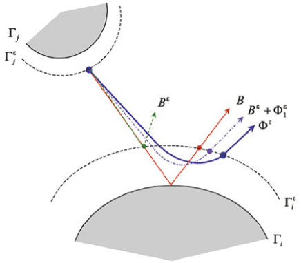
Figure 7: Billiard map $B$ (red). Billiard map of the auxiliary billiard $B^{\epsilon}$ (green). Poincaré map for the smooth Hamiltonian flow $\Phi^{\epsilon}$ (blue). The first approximation of $\Phi^{\epsilon}$ $B^{\epsilon}+\Phi_{1}^{\epsilon}$ (violet).

Combining the above lemmas we establish:

Theorem 3.

Let the potential $V(q;\epsilon)$ satisfy Conditions I-IV, and choose $\delta_{i}$’s and $\nu_{i}$’s such that $\delta_{i}(\epsilon),\nu_{i}(\epsilon),m^{(r)}(\epsilon),M_{i}^{(r)}(\epsilon)\rightarrow 0$ as $\epsilon\rightarrow 0$. Then, on the cross-section $S_{\epsilon}$ (see (26)) near orbits of a regular reflection, for all sufficiently small $\epsilon$ the Poincaré map $\Phi^{\epsilon}$ of the smooth Hamiltonian flow is defined, and it is $O(m^{(r)}+\nu+M^{(r)})$-close in the $C^{r}$-topology to the billiard map $B^{\epsilon}=R_{\circ}^{\epsilon}\circ F_{\circ}^{\epsilon}$ in the auxiliary billiard table $D^{\epsilon}$ (see Figure 7). Furthermore,

$$\Phi^{\epsilon}=R^{\epsilon}\circ F^{\epsilon}=B^{\epsilon}+O_{{}_{C^{r}}}(m^{(r)}+\nu+M^{(r)})=(R_{\circ}^{\epsilon}+R_{1}^{\epsilon})\circ(F_{\circ}^{\epsilon}+F_{1}^{\epsilon})+O_{{}_{C^{r-1}}}((m^{(r)}+\nu+M^{(r)})^{2})\\ =:B^{\epsilon}+\Phi_{1}^{\epsilon}+O_{{}_{C^{r-1}}}((m^{(r)}+\nu+M^{(r)})^{2})$$ (40)

(where $\nu=\max_{i}\nu_{i}$, $M^{(r)}=\max_{i}M_{i}^{(r)}$,$\Phi_{1}^{\epsilon}=O_{{}_{C^{r-1}}}(m^{(r)}+\nu+M^{(r)})$, and the first order corrections $F_{1}^{\epsilon}$ and $R_{1}^{\epsilon}$ are explicitly calculated in Lemmas 2 and 3).

Theorem 4.

Given a finite $T$ and a regular billiard trajectory in $[0,T]$, the time $t$ map of the smooth Hamiltonian flow and of the corresponding auxiliary billiard are $O(\nu+m^{(r)}+M^{(r)})$-close in the $C^{r}$-topology for all $t\in T\backslash T_{R}$, where $T_{R}$ is the finite collection of impact intervals each of them of length $O(|\delta|+M^{(r)})$.

3.3.1 Error estimates for some model potentials

Now we can estimate the deviation of the smooth Hamiltonian trajectories from the regular (non-tangent, non-corner) billiard ones for various concrete potentials $V(q;\epsilon)$. To make a general estimate possible, we have to assume that the behavior of the potential near the boundary dominates the estimate; We say that $V(q;\epsilon)$ is boundary dominated, if $V(q;\epsilon)$ and its derivatives are smaller in the interior of $D_{int}^{\epsilon}$ (i.e. in the region bounded by the surfaces $Q(q;\epsilon)=Q_{i}+\delta_{i}(\epsilon)$) than on the boundary of this domain. This means that for boundary dominated potentials

$$m^{(r)}(\delta;\epsilon)=\sup_{{\footnotesize\begin{array}[c]{c}q\in D_{int}^{\epsilon}\\ 1\leq l\leq r+1\end{array}}}\|\partial^{l}V(q;\epsilon)\|=\sup_{{\footnotesize\begin{array}[c]{c}q\in\partial D_{int}^{\epsilon}\\ 1\leq l\leq r+1\end{array}}}\|\partial^{l}V(q;\epsilon)\|.$$ (41)

By the definition of the pattern function $Q$, near a given boundary $\Gamma_{i}$

$$V(q;\epsilon)\bigg{|}_{q\in\partial D_{int}^{\epsilon}}\equiv W_{i}(Q(q;\epsilon)-Q_{i};\epsilon)\bigg{|}_{Q=Q_{i}+\delta_{i}}=W_{i}(\delta_{i};\epsilon)$$

Since $Q(q;\epsilon)$ is bounded with its derivatives, we conclude that there exists a constant $C$ such that

$$m^{(r)}(\delta;\epsilon)=C\max_{i}\max_{{\footnotesize 1\leq l\leq r+1}}|W_{i}^{(l)}(\delta_{i};\epsilon)|.$$ (42)

Thus, for boundary dominated potentials, one can estimate the differences $h_{t}^{\epsilon}-b_{t}$ and $\Phi^{\epsilon}-B^{\epsilon}$ in terms of the barrier functions alone.

The corresponding estimates given by Theorems 4 and 3 hold true for every choice of $\nu$ and $\delta$ such that $\delta(\epsilon),\nu(\epsilon),m_{r}(\delta(\epsilon);\epsilon),M_{r}(\nu(\epsilon);\epsilon)\rightarrow 0$ as $\epsilon\rightarrow 0$ (for simplicity of notation we assume hereafter that the barrier function $W$ is the same for all boundary surfaces $\Gamma_{i}$, and thus suppress the dependence on $i$). To obtain the best estimates, we have to find $\nu(\epsilon)$ and $\delta(\epsilon)$ which minimize the expression $\nu+M^{(r)}(\nu;\epsilon)+m^{(r)}(\delta;\epsilon)$. In this way, we first find $\nu(\epsilon)$ which minimizes $\nu+M^{(r)}(\nu;\epsilon)$. As $M^{(r)}$ is a decreasing function of $\nu$ (see (22)), the sought $\nu(\epsilon)$ solves the equation

$$\nu=M^{(r)}(\nu;\epsilon).$$ (43)

After $\nu$ is determined, we may try to make $\delta(\epsilon)$ go to zero so slow that the corresponding value of $m^{(r)}$ (see (42)) will be asymptotically equal to $\nu(\epsilon)$. Once succeeded, we may conclude that $\nu(\epsilon)$ given by (43) estimates the deviation between regular billiard and smooth trajectories. Notice that the significance of $\nu(\epsilon)$ is three-folded; First, it determines the optimal auxiliary billiard which supplies the best approximation to the smooth Hamiltonian flow (see Lemma 3). Second, it estimates the accuracy of this approximation. Third, it determines, via the relation $m^{(r)}(\delta)=\nu$, the width $|\delta(\epsilon)|+\nu(\epsilon)$ of the boundary layer in which the billiard and the Hamiltonian flows are not close (Theorem 4). Let us proceed to examples.

Proposition 1.

Consider the boundary dominated potential $V(q;\epsilon)$ corresponding to the barrier function $W(Q)=e^{-\frac{Q}{\epsilon}}$ for small $Q$. Then, near regular billiard trajectories, the smooth Hamiltonian flow is $O(\sqrt[r+2]{\epsilon})$-close in the $C^{r}$-topology to the billiard flow within the auxiliary billiard defined by the level set $Q(q;\epsilon)=\eta(\epsilon)=O(\epsilon\ln\epsilon)$. The corresponding Poincaré map $\Phi^{\epsilon}$ is $O_{{}_{C^{r}}}(\sqrt[r+2]{\epsilon})$-close to the auxiliary billiard map $B^{\epsilon}$. The impact intervals lengths are $O(\sqrt[r+2]{\epsilon})$.

Proof.

Since $W^{(l)}(Q;\epsilon)=(-\epsilon)^{-l}e^{-\frac{Q}{\epsilon}}$, we obtain that $m^{(r)}(\delta;\epsilon)=O(\epsilon^{-(r+1)}e^{-\frac{\delta}{\epsilon}})$ (since the potential is boundary dominated, we may use (42)). The inverse to $W(Q;\epsilon)$ is given by $\mathcal{Q}(W;\epsilon)=-\epsilon\ln W$, so $\mathcal{Q}^{(l)}(W;\epsilon)=(-1)^{l}(l-1)!\epsilon W^{-l}$, and $M^{(r)}(\nu,\epsilon)=O(\epsilon\nu^{-{(r+1)}})$ (see (22)). Plugging this in (43), we find

$$\nu(\epsilon)=\sqrt[r+2]{\epsilon}.$$ (44)

By choosing $\delta(\epsilon)=-(r+1+\frac{1}{r+2})\epsilon\ln\epsilon$, we obtain $m^{(r)}(\delta,\epsilon)\sim\nu(\epsilon)$, so for $\nu$ given by (44) we have that $\nu+M^{(r)}+m^{(r)}=O(\nu)$, and the proposition now follows immediately from Theorems 3 and 4 (the value of $\eta(\epsilon)=O(\epsilon\ln\epsilon)$ is given by $\eta=\mathcal{Q}(\nu;\epsilon)$). ∎

Proposition 2.

Let the boundary dominated potential $V(q;\epsilon)$ correspond to the barrier function $W(Q)=e^{-\frac{Q^{2}}{\epsilon}}$ for small $Q$. Then, near the regular billiard trajectories, the smooth Hamiltonian flow is $O(\nu(\epsilon))=O(\sqrt[2(r+2)]{\frac{\epsilon}{|\ln\epsilon|}})$-close in the $C^{r}$-topology to the billiard flow within the auxiliary billiard defined by the level set $Q(q;\epsilon)=\eta(\epsilon)=O(\sqrt{\epsilon|\ln\epsilon|})$. The corresponding Poincaré map $\Phi^{\epsilon}$ is $O_{{}_{C^{r}}}(\nu(\epsilon))$-close to the auxiliary billiard map $B^{\epsilon}$. The impact intervals are of the length $O(\nu(\epsilon))$.

Proof.

It is easy to see that $W^{(l)}(Q;\epsilon)=O((\frac{Q}{\epsilon})^{l}e^{-\frac{Q^{2}}{\epsilon}})$ for $Q\gg\sqrt{\epsilon}$, hence $m^{(r)}(\delta;\epsilon)=O((\frac{\delta}{\epsilon})^{r+1}e^{-\frac{\delta^{2}}{\epsilon}})$. From $\mathcal{Q}(W;\epsilon)=\sqrt{-\epsilon\ln W}$ we obtain $M^{(r)}(\nu;\epsilon)=O(\sqrt{\frac{\epsilon}{|\ln\nu|}}\nu^{-(r+1)})$. Plugging this in (43), we indeed find

$$\nu(\epsilon)=M^{(r)}(\nu;\epsilon)=O(\sqrt[2(r+2)]{\frac{\epsilon}{|\ln\epsilon|}}),$$

as required. By choosing $\delta(\epsilon)\sim\sqrt{-\frac{1}{2}(r+1+\frac{1}{r+2})\epsilon\ln\epsilon}$, we obtain $m^{(r)}(\delta;\epsilon)\sim\nu(\epsilon)$, so the rest follows directly from Theorems 3 and 4. ∎

Proposition 3.

Let the boundary dominated potential $V(q;\epsilon)$ correspond to the barrier function $W(Q)=(\frac{\epsilon}{Q})^{\alpha}$. Then, near the regular billiard trajectories, the smooth Hamiltonian flow is $O(\nu(\epsilon))=O(\sqrt[r+2+\frac{1}{\alpha}]{\epsilon})$-close in the $C^{r}$-topology to the billiard flow within the auxiliary billiard defined by the level set $Q(q;\epsilon)=\eta(\epsilon)=O(\nu^{r+2})$. The corresponding Poincaré map $\Phi^{\epsilon}$ is $O_{{}_{C^{r}}}(\nu(\epsilon))$-close to the auxiliary billiard map $B^{\epsilon}$. The impact intervals are $O(\nu(\epsilon))$ when $\alpha\geq 1$, and $O(\nu(\epsilon)^{\frac{\alpha(r+2)}{\alpha+r+1}})$ when $\alpha\leq 1$.

Proof.

As above, using $W^{(l)}(Q;\epsilon)=O(\frac{\epsilon^{\alpha}}{Q^{l+\alpha}})$ we obtain that $m^{(r)}(\delta;\epsilon)=O(\frac{\epsilon^{\alpha}}{\delta^{r+1+\alpha}})$, and since $\mathcal{Q}(W;\epsilon)=\frac{\epsilon}{W^{1/\alpha}}$, we find $\mathcal{Q}^{(l)}(W;\epsilon)=O(\frac{\epsilon}{W^{l+1/\alpha}})$ and thus $M^{(r)}(\nu;\epsilon)=O(\frac{\epsilon}{\nu^{r+1+1/\alpha}}).$ It follows that $\nu(\epsilon)=O(\sqrt[r+2+\frac{1}{\alpha}]{\epsilon})$ solves $\nu=M^{(r)}(\nu;\epsilon)$. Now $\eta(\epsilon)=\mathcal{Q}(\nu)=\frac{\epsilon}{\nu^{1/\alpha}}=O(\nu^{r+2})$. By taking $\delta(\epsilon)=\nu^{\frac{\alpha(r+2)}{r+1+\alpha}}$, we ensure that $m^{(r)}(\delta,\epsilon)\sim\nu(\epsilon)$. The length of impact intervals is now given by $O(\nu+\delta)$. ∎

Note that the asymptotic for the deviation of the smooth trajectories from the billiard ones and for the length of the impact intervals depend strongly on $r$, i.e. on the number of derivatives (with respect to initial conditions) which we want to control.

3.4 Persistence of periodic and homoclinic orbits

The closeness of the billiard and smooth flows after one reflection leads, using standard results, to persistence of regular periodic and homoclinic orbits. For completeness we state these results explicitly:

Theorem 5.

Consider a Hamiltonian system with a potential $V(q,\epsilon)$ satisfying Condition I-IV in a billiard table $D$. Let $P^{b}(t)$ denote a non-parabolic, non-singular periodic orbit of a period $T$ for the billiard flow. Then, for any choice of $\nu(\epsilon),\delta(\epsilon)$ such that $\nu(\epsilon),\delta(\epsilon),m^{(1)}(\epsilon),M^{(1)}(\epsilon)\rightarrow 0$ as $\epsilon\rightarrow 0$, the smooth Hamiltonian flow has a uniquely defined periodic orbit $P^{\epsilon}(t)$ of period $T^{\epsilon}=T+O(\nu+m^{(1)}+M^{(1)})$, which stays $O(\nu+m^{(1)}+M^{(1)})$-close to $P^{b}$ for all $t$ outside of collision intervals (finitely many of them in a period) of length $O(|\delta|+M^{(1)})$. Away from the collision intervals, the local Poincaré map near $P^{\epsilon}$ is $O_{{}_{C^{r}}}(\nu+m^{(r)}+M^{(r)})$-close to the local Poincaré map near $P^{b}$. In particular, if $P^{b}$ is hyperbolic, then $P^{\epsilon}$ is also hyperbolic and, inside $D^{\epsilon}$, the stable and unstable manifolds of $P^{\epsilon}$ approximate $O_{{}_{C^{r}}}(\nu+m^{(r)}+M^{(r)})$-closely the stable and unstable manifolds of $P^{b}$ on any compact, forward-invariant or, respectively, backward-invariant piece bounded away from the singularity set in the billiard’s phase space; furthermore, any transverse regular homoclinic orbit to $P^{b}$ is, for sufficiently small $\epsilon$, inherited by $P^{\epsilon}$ as well.

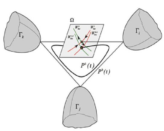
Figure 8: $P^{b}$ is a billiard periodic orbit (solid). $P^{\epsilon}$ is a periodic orbit of the smooth Hamiltonian flow (bold).

As $P^{b}$ is a regular periodic orbit, i.e. it makes only regular reflections from the boundary (a finite number of them on the period), it follows from Theorem 3 that a Poincaré map for the smooth Hamiltonian flow near $P^{b}$ is $O(\nu+m^{(1)}+M^{(1)})$-close in $C^{1}$ topology to the Poincaré map of the auxiliary billiard $D^{\epsilon}$, while the latter is $O(\eta(\epsilon))$-close to the Poincaré map for the original billiard $D$. Moreover, from (22) it follows that $\eta(\epsilon)\leq M^{(0)}\leq M^{(1)}$ and we can conclude that a Poincaré map for the smooth Hamiltonian flow near $P^{b}$ is $O(\nu+m^{(1)}+M^{(1)})$-close in $C^{1}$ topology to the Poincaré map for the original billiard $D$. Since, by assumption, $P^{b}(t)$ is non-parabolic, the corresponding fixed point of the Poincaré map persists for sufficiently small $\epsilon$ in virtue of the implicit function theorem (the closeness of the corresponding continuous-time orbits is given by Theorem 4). The continuous dependence of the invariant manifolds of $\epsilon$ in the hyperbolic case follows from the continuous dependence of the Poincaré map $\Phi^{\epsilon}$ on $\epsilon$ at all $\epsilon\geq 0$ (Theorem 3), and implies the persistence of transverse homoclinics immediately. Indeed, the formulation regarding the closeness of compact pieces of the global stable and unstable manifolds may be easily verified by applying finite time extensions of the local stable and unstable manifolds. Note that similar persistence result holds true for topologically transverse homoclinic orbits.

More generally, one may claim (by the shadowing lemma) the persistence of compact uniformly hyperbolic sets composed of regular billiard orbits. Note that the accuracy of the approximation of smooth orbits (periodic and aperiodic) by the billiard ones, does not depend on the orbit (e.g. is independent of its period) and is given by the maximal deviation for each reflection (times a constant). This holds true for any compact set of regular orbits of a strictly dispersing billiard flow (since such billiards are uniformly hyperbolic); see for example a nice application by Chen [9].

In some cases, to establish the existence of transverse or topologically transverse homoclinic orbits in a family of billiard flows $b_{t}(\gamma)$ in $D_{\gamma}$, one uses higher dimensional generalizations of the Poincare-Melnikov integral (see Section 4). In particular, with the near integrable setting, the ”splitting distance” between the manifolds near the transverse homoclinic orbit may be proportional to an unfolding parameter $\gamma$. The above theorem implies that if $\epsilon_{0}=\epsilon_{0}(\gamma)$ is chosen so that $\nu(\epsilon_{0},\gamma)+m^{(1)}(\delta(\epsilon_{0},\gamma);\epsilon_{0},\gamma)+M^{(1)}(\nu(\epsilon_{0},\gamma);\epsilon_{0},\gamma))=o(\gamma)$ and $\epsilon_{0}(\gamma)\rightarrow 0$ as $\gamma\rightarrow 0$ then, for sufficiently small $\gamma$, transverse homoclinic orbits appear in the smooth flow for all $\epsilon\in(0,\epsilon_{0}(\gamma))$. In the next section we use this remark and [11] to establish that transverse homoclinic orbits appear in families of smooth billiard potentials which limit to the ellipsoidal billiard.

4 Application to ellipsoidal billiards with potential

Consider the billiard motion in an ellipsoid

$$D=\{q\in\mathbb{R}^{n}:\langle q,A^{-2}q\rangle\leq 1\},$$ (45)

$$A=\operatorname{diag}(d_{1},\ldots,d_{n})\;\;\;\;\;\;\;d_{1}\geq\ldots\geq d_{n}\geq 0.$$

The ellipsoid is called generic if all the above inequalities are strict. A well known result of Birkhoff [3] is that the billiard motion in an ellipsoid is integrable, and the mathematical theory which may be invoked to describe and generalize this result is still under development - see Radnovic [16] and references therein. Delshams et al [11] and recently Bolotin et al [4] (see also references therein) investigate when small non-quadratic symmetric perturbations to the ellipsoidal shape change the integrability property. In this series of works the authors prove the persistence of some symmetric homoclinic orbits, and for specific cases they prove that these orbits are transverse homoclinic orbits of the perturbed billiard, thus proving that integrability is destroyed. Here, we show that using the machinery we developed we can immediately extend their work to the smooth billiard-potential case (notice that in [4] some results are extended to billiards with a $C^{2}$-small Hamiltonian perturbation in the domain’s interior, however the billiard potentials which we consider do not fall into this category - near the boundary they correspond to a large perturbation even in the $C^{1}$-norm). We will first explain the relevant main results of Delshams et al, then supply the corresponding proposition for the smooth case (consequences of Theorem 2, or more specifically of Theorem 5) and then the corresponding quantitative estimates for specific potentials (which follows from Propositions 1-3).

4.1 The billiard in a perturbed ellipsoid

Consider the simplest unstable periodic orbit in an ellipsoidal billiard - the orbit along the diameter of the ellipsoid joining the vertices $(-d_{1},0,\ldots,0)$ and $(d_{1},0,\ldots,0).$ Denote the set formed by the two-periodic points associated with the diameter by

$$P^{b}=\{\rho_{+},\rho_{-}\}\quad\rho_{\pm}=\{q_{\pm},p_{\mp}\}\quad q_{\pm}=(\pm d_{1},0,\ldots,0)\quad p_{\pm}=(\pm 1,0,\ldots,0).$$ (46)

These points correspond to isolated two-periodic hyperbolic orbits of the Billiard map $B$ and the corresponding periodic orbit $P_{t}^{b}=b_{t}(\rho_{+})$ of the billiard flow. The $n-1$-dimensional ($n$-dimensional for the flow) stable and unstable manifolds of this periodic orbit coincide; In $2$-dimensions there are 4 separatrices connecting $\{\rho_{+},\rho_{-}\}$ whereas the topology of the separatrices in the higher dimensional case is non-trivial - it is well described by CW complexes for the 3 dimensional case and by hierarchal structure of separatrix submanifolds in the higher dimensional case (see [11]).

Of specific interest are the symmetric homoclinic orbits - it is established in [11] that in the generic $2$ dimensional case there are exactly $4$ homoclinic orbits which are $x-$symmetric (symmetric, in the configuration space, to reflections about the $x$-axis) and $4$ which are $y-$symmetric. In the generic $3$ dimensional case, in addition to the $16$ planar symmetric orbits ($8$ in each of the symmetry planes- $xy$ and $xz$) there are $16$ additional symmetric spatial orbits - $8$ are symmetric with respect to reflection about the $xz$ plane and $8$ are $y$ axial. In the $n$ dimensional case there are $2^{n+1}$ spatial symmetric orbits.

Denote by $P^{b-\hom}=\left\{P_{i}^{b-\hom}\right\}_{i=-\infty}^{\infty}$ one of these symmetric homoclinic orbits of the billiard map in the ellipsoid, so $P_{i+1}^{b-\hom}=BP_{i}^{b-\hom}$ and $P_{t}^{b-\hom}=b_{t}(P_{0}^{b-\hom})$ denotes the corresponding continuous orbit of the billiard flow. Given a $\varsigma$ such that $0<\varsigma\ll d_{n}$, define the local cross-sections of the billiard map by:

$$\Sigma^{-} =\{(q,p)|q\in\partial D,q_{1}+d_{1}<\varsigma,\text{ }1-p_{1}<\varsigma\},$$

$$\Sigma^{+} =\{(q,p)|q\in\partial D,d_{1}-q_{1}<\varsigma,\text{ }p_{1}+1<\varsigma\},$$

so, in particular, $\rho_{\pm}\in$ $\Sigma^{\pm}$ and $\Sigma^{\pm}\subset S$, where $S$ is the natural cross-section on which the billiard map is defined (see Section 2.2). It follows that only a finite number of points in $P^{b-\hom}$ do not fall into $\Sigma^{\pm}$, and that for any given geometry there exist a finite $\varsigma$ such that $P^{b-\hom}\backslash\{P^{b-\hom}\cap\Sigma^{\pm}\}\neq\varnothing$ for all the symmetric orbits. See Figure 9. Thus, it is possible to choose $P_{0}^{b-\hom}$ and a local cross-section $\Sigma^{0}$ such that $P_{0}^{b-\hom}\in\Sigma^{0}\subset\{S\backslash\{\Sigma^{+}\cup\Sigma^{-}\}\}$. Notice that for the ellipsoid all the reflections are regular, and furthermore, for the symmetric homoclinic orbits, if $d_{1}$ is finite and $d_{n}$ is positive then all the reflection angles of $P^{b-\hom}$ are strictly bounded away from $\pi/2$.

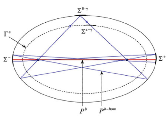
Figure 9: Billiard trajectory giving rise to a y-symmetric homoclinic orbit (blue).

Now, consider a symmetric perturbation of the ellipsoid $Q$ of the form:

$$D_{\gamma}=\{q\in\mathbb{R}^{n}:\langle q,A^{-2}q\rangle\leq 1+\gamma\Xi(\frac{q_{1}^{2}}{d_{1}^{2}},\ldots,\frac{q_{n}^{2}}{d_{n}^{2}})\},$$ (47)

where the hypersurface $D_{\gamma}\in\mathbb{R}^{n+1}$ is symmetric with regard to all the coordinate axis of $\mathbb{R}^{n}$ and the function $\Xi:\mathbb{R}^{n}\rightarrow\mathbb{R}$ is either a general entire function, such that $\Xi(0,\ldots,0)=0$ or of a specific form (e.g. quadratic). By using symmetry arguments, Delshams et al [11] prove that for generic billiard the above mentioned symmetric homoclinic orbits persist under such symmetric perturbations. Furthermore, analyzing the asymptotic properties of the symplectic discrete version of the Poincaré-Melnikov potential (the high dimensional analog of the integral), they prove that for sufficiently small perturbations (small $\gamma$) the $n$-dimensional symmetric homoclinic orbits are transverse in the following four cases:

1. In two-dimensions, for narrow ellipses ($\beta_{1}=\frac{d_{2}^{2}}{d_{1}^{2}}\ll 1$), for any analytic small enough symmetric perturbation.

2. In two-dimensions, in the non-circular case ($\beta_{1}\neq 1$), for $\Xi(\frac{x^{2}}{d_{1}^{2}},\frac{y^{2}}{d_{2}^{2}})=\frac{y^{4}}{d_{2}^{4}}$.

3. In the three-dimensional case, for nearly flat ellipses ($\beta_{2}=\frac{d_{3}^{2}}{d_{1}^{2}}\ll 1$), for perturbations of the form: $\Xi(\frac{x^{2}}{d_{1}^{2}},\frac{y^{2}}{d_{2}^{2}},\frac{z^{2}}{d_{3}^{2}})=\frac{z^{2}}{d_{3}^{2}}R(\frac{y^{2}}{d_{2}^{2}},\frac{z^{2}}{d_{3}^{2}})$ where $R$ is a generic polynomial (or of some specific list).

4. In the three-dimensional case, for nearly oblate ellipses ($\beta_{1}=\frac{d_{2}^{2}}{d_{1}^{2}}\simeq 1$), for the perturbation $\Xi(\frac{x^{2}}{d_{1}^{2}},\frac{y^{2}}{d_{2}^{2}},\frac{z^{2}}{d_{3}^{2}})=\frac{z^{2}}{d_{3}^{2}}\frac{y^{2}}{d_{2}^{2}}$.

To establish these results, the Poincaré-Melnikov potential is calculated for each of these cases, and it is shown that it has non-degenerate critical points at the corresponding symmetric trajectories. It follows that $P^{b-\hom-\gamma}$ persists and the change in the splitting distance between the separatrices $\mathcal{W}^{u}$ and $\mathcal{W}^{s}$ near $P_{0}^{b-\hom-\gamma}$ is proportional to $\gamma$, the perturbation amplitude, so that near $P_{0}^{b-\hom-\gamma}$ at the local cross-section $\Sigma^{0-\gamma}$,

$$d(W_{\gamma}^{s},W_{\gamma}^{u})=M(r)\gamma+O(\gamma^{2}).$$ (48)

where $r\in R^{n-1}$ denotes some parametrization along $\mathcal{W}$ and $M(r)$ (the gradient of the Poincaré-Melnikov potential) has simple zeroes at the parameter values corresponding to any of the spatial symmetric homoclinic orbits $P_{0}^{b-\hom}$.

4.2 Smooth Potential in a near ellipsoidal region

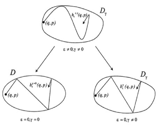
Figure 10: Perturbation of a billiard flow inside a perturbed ellipsoid family $D_{\gamma}$.

Let us now consider a two parameter family of smooth potentials $V(q;\gamma,\epsilon)$ which limit, as $\epsilon\rightarrow 0$ to the billiard flow in the perturbed ellipsoid family $D_{\gamma}$; namely, consider the family of Hamiltonian flows:

$$H(\epsilon,\gamma)=\frac{p^{2}}{2}+V(q;\gamma,\epsilon).$$ (49)

where $V(q;\gamma,\epsilon)$ satisfies conditions I-IV for all $\gamma$ values. In the four cases mentioned above, the flow limits, as $\epsilon\rightarrow 0,$ to an integrable billiard motion inside the ellipsoid $D$ when $\gamma=0$ and, for $\gamma\neq 0,$ to a non-integrable billiard motion inside the perturbed ellipsoid $D_{\gamma}$. See Figure 10.

Applying Theorem 5 to an interior transverse local return map near $\Sigma^{0-\gamma}$, and noticing that all homoclinic orbits of the billiard flow in $D_{\gamma}$ are regular orbits, we immediately establish:

Proposition 4.

Consider the Hamiltonian flow (49), where $V(q;\gamma,\epsilon)$ is a billiard potential limiting to the billiard flow in $D_{\gamma}$ ($V(q;\gamma,\epsilon)$ satisfies conditions I-IV for all $\gamma$ values). Let the function $\epsilon_{0}(\gamma)$ satisfy

$$\nu(\epsilon_{0},\gamma)+m^{(1)}(\delta(\epsilon_{0},\gamma);\epsilon_{0},\gamma)+M^{(1)}(\nu(\epsilon_{0},\gamma);\epsilon_{0},\gamma))=o(\gamma)$$

and $\epsilon_{0}(\gamma)$ $\rightarrow 0$ as $\gamma\rightarrow 0$. Then, for each of the above cases 1-4, for sufficiently small $\gamma>0$, the smooth flow has transverse homoclinic orbits which limit to the billiard’s transverse homoclinic orbits for all $0<\epsilon<\epsilon_{0}(\gamma)$.

Indeed, for sufficiently small $\gamma>0$ equation (48) is valid, and thus the homoclinic billiard orbit $P^{b-\hom-\gamma}$ is transverse, so the above theorem follows immediately from Theorem 5 and the discussion after it. Based on this proposition and Propositions 1-3 we conclude:

Proposition 5.

Consider the Hamiltonian flow (49), where $V(q;\gamma,\epsilon)$ is a billiard potential limiting to the billiard flow in $D_{\gamma}$ ($V(q;\gamma,\epsilon)$ satisfies conditions I-IV for all $\gamma$ values). Further assume that the potential $V(q;\gamma,\epsilon)$ is boundary dominated and is given near the boundary of $D_{\gamma}$ by $W(Q;\epsilon),$ so that (41) holds for the corresponding $\delta$ values which are specified bellow. Then, for each of the above cases 1-4, for sufficiently small $\gamma>0$, the smooth flow has transverse homoclinic orbits which limit to the billiard’s transverse homoclinic orbits and thus is non-integrable for all $0<\epsilon<\epsilon_{0}(\gamma)$, where

• For $W(Q;\epsilon)=e^{-\frac{Q}{\epsilon}}$ : $\delta=O(-\epsilon\ln\epsilon)$ and $\epsilon_{0}(\gamma)=\gamma^{3+\varkappa},\varkappa>0.$

• For $W(Q;\epsilon)=e^{-\frac{Q^{2}}{\epsilon}}$ : $\delta=O(\sqrt{-\epsilon\ln\epsilon})$ and $\epsilon_{0}(\gamma)=\gamma^{6+\varkappa},\varkappa>0.$

• For $W(Q;\epsilon)=(\frac{\epsilon}{Q})^{\alpha}$ : $\delta=O(\sqrt[3+\frac{1}{\alpha}]{\epsilon})$ and $\epsilon_{0}(\gamma)=\gamma^{3+\frac{1}{\alpha}+\varkappa},\varkappa>0$.

5 Discussion

The paper includes three main results:

• Theorems 1-2 deal with the smooth convergence of flows in steep potentials to the billiard’s flow in the multi-dimensional case. These results, which are a natural extension of [35], provide a powerful theoretical tool for proving the persistence of various billiard trajectories in the smooth systems, and vice versa. The unavoidable emergence of degenerate tangencies in the higher dimensional setting, and the study of corners and regular tangencies (extending [27],[36] to higher dimensions) have yet to be addressed.

• Theorems 3-4 provide the first order corrections for approximating the smooth flows by billiards for regular reflections. Theorem 3 proposes the appropriate zeroth order billiard geometry which best approximates the steep billiard and a simple formula for computing the first order correction terms, thus allowing to study the effect of smoothing. The smooth flow and the billiard flow do not match in a boundary layer - the width of it and the time spent in it are specified in Theorem 4. Propositions 1-3 supply the estimates for the boundary layer width and the accuracy of the auxiliary billiard approximation for some typical potentials (exponential, Gaussian and power-law). All these results are novel for any dimension, and propose a new approach for studying problems with relatively steep potentials. A plethora of questions regarding the differences between the smooth and hard wall systems can now be rigorously analyzed.

• Theorem 5 and Proposition 5: The above mentioned $C^{1}$ estimates of the error terms lead naturally to the persistence Theorem 5. Applying these results to the billiards studied in [11], we prove that the motion in steep potentials in various deformed ellipsoids are non-integrable for an open interval of the steepness parameter, and we provide a lower bound for this interval length for the above mentioned typical potentials. While the analysis of higher dimensional Hamiltonian systems is highly non-trivial, we demonstrate here that some results which are obtained for maps may be immediately extended to the smooth steep case. We note that the same statement works in the opposite direction. Furthermore, one may use the first order corrections developed in Theorem 3 and Propositions 1-3 to study the possible appearance of non-integrabilty due to the introduction of smooth potentials.

As mentioned before, these results may give the impression that the smooth flow and the billiard flow are indeed very similar. While in this work we emphasize the closeness of the two flows, it is important to bear in mind that this is not the case in general. This observation applies to the local behavior near solutions which are not structurally stable and is especially important when dealing with asymptotic properties such as ergodicity, as discussed below.

Let us first remark about the local behavior. First, as in the two-dimensional settings, we expect that singular orbits or polygons of the billiard give rise to various types of orbits in the smooth setting. The larger the dimension of the system, the larger is the variety of orbits which may emerge from these singularities. Moreover, in this higher dimensional setting, even though our theory implies that regular elliptic or partially-elliptic periodic orbits persist, the motion near them (and their stability) may change.

Global properties of the phase space are even more sensitive to small changes. If the billiard periodic orbit is hyperbolic, while it and its local stable and unstable manifolds persist (see for example Theorem 5), their global structure in the smooth case may be quite different; First of all, integrability of one of the systems does not imply integrability of the other (for example, it may be possible to use the correction terms computed in Section 3.3 to establish that the smooth flow has separatrix splitting even when the billiard is integrable). Second, if the billiard flow has singularities, the global manifolds of a hyperbolic billiard orbit may have discontinuities and singularities whereas the global manifolds of the smooth orbit are smooth (see for example [35]).

Finally, the most celebrated global property one is interested in is ergodicity and mixing. Indeed, Boltzmann suggested that the gas molecules interacting in a box should have a fast decaying correlation function and proposed the analogy of the corresponding dispersing hard balls system. In modern terminology, Boltzmann claimed that for sufficiently large systems the hard sphere gases are ergodic and mixing [21] and hence so are the real gases. Sinai [29] proved that the dispersion property is sufficient for proving that the system of two disks on a two-torus is ergodic and mixing, and following this fundamental work the study of the dynamics and mixing properties in various two-dimensional billiard tables had flourished [5, 6, 38, GarGal94] (the behavior of billiards in higher dimensions is much less studied, see [39, 8, 7, 26][31][28] and references therein).

The suspicion that the motion in smooth steep potentials may have a different character has been lurking all along. In fact, several works where dedicated to proving that in some cases (finite-range axis-symmetric potentials) the motion may be still ergodic [29, 22, 23, 15, 2]. In [14] it was shown that when two particles with a finite range potential move on a two-dimensional torus stable periodic orbit may emerge. In [35] we proved that in the two dimensional case ($C^{r}$ smooth potentials, not necessarily finite range, not necessarily symmetric), near singular trajectories (tangent trajectories or corner trajectories) new islands of stability are born in the smooth flow for arbitrarily steep potentials. Thus there is a fundamental difference in the ergodic properties of hard-wall potentials as compared to smooth potentials. Although these results only apply to two-particle systems, they raise the possibility that systems with large numbers of particles interacting by smooth potentials could also be non-ergodic. The tools developed here may be useful in studying these possibilities.

6 Acknowledgments

This research is supported by the Israel Science Foundation (Grant no. 926/04) and by the Minerva foundation.

7 Appendix

7.1 Proof of Theorems 1 and 2

By Condition I the Hamiltonian flow is $C^{r}$-close to the billiard flow outside an arbitrarily small boundary layer. So we will concentrate our attention on the behavior of the Hamiltonian flow inside such a layer.

Let the initial conditions correspond to the billiard orbit which hits a boundary surface $\Gamma_{i}$ at a (non-corner) point $q_{c}$. By Condition IIa, the surface $\Gamma_{i}$ is given by the equation $Q(q;0)=Q_{i}$, hence the boundary layer near $\Gamma_{i}$ can be defined as $N_{\delta}=\{|Q(q;\epsilon)-Q_{i}|\leq\delta\}$, where $\delta$ tends to zero sufficiently slowly as $\epsilon\rightarrow+0$. Take $\epsilon$ sufficiently small. The smooth trajectory enters $N_{\delta}$ at some time $t_{in}(\delta,\epsilon)$ at a point $q_{in}(\delta,\epsilon)$ which is close to the collision point $q_{c}$ with the velocity $p_{in}(\delta,\epsilon)$ which is close to the initial velocity $p_{0}$. See Figure 11. The same trajectory exits from $N_{\delta}$ at the time $t_{out}(\delta,\epsilon)$ at a point $q_{out}(\delta,\epsilon)$ with velocity $p_{out}(\delta,\epsilon)$. In these settings, the theorems are equivalent ($r=0$ corresponds to Theorem 1, while $r>0$ corresponds to Theorem 2) to proving the following statements:

$$\lim_{\delta\rightarrow 0}\lim_{\epsilon\rightarrow+0}\bigg{\|}\bigg{(}q_{out}(\delta,\epsilon),t_{out}(\delta,\epsilon)\bigg{)}-\bigg{(}q_{in}(\delta,\epsilon),t_{in}(\delta,\epsilon)\bigg{)}\bigg{\|}_{C^{r}}=0,$$ (50)

which guarantees that the trajectory does not travel along the boundary, and (see (5))

$$\lim_{\delta\rightarrow 0}\lim_{\epsilon\rightarrow+0}\bigg{\|}p_{out}(\delta,\epsilon)-p_{in}(\delta,\epsilon)+2n(q_{in})\langle p_{in}(\delta,\epsilon),n(q_{in})\rangle\bigg{\|}_{C^{r}}=0,$$ (51)

where $n(q)$ is the unit inward normal to the level surface of $Q$ at the point $q$.

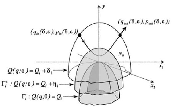
Figure 11: Hamiltonian flow inside small boundary layer.

With no loss of generality, assume that $Q(q;0)$ increases as $q$ leaves $D^{\prime}s$ boundary towards $D^{\prime}s$ interior. Choose the coordinates $(x,y)$ so that the hyperplane $x$ is tangent to the level surface $Q(q;\epsilon)=Q(q_{c};\epsilon)$ and the $y$-axis is the inward normal to this surface at $q=q_{c}$. Hence, the partial derivatives of $Q$ satisfy:

$$Q_{x}|_{(q_{c};\epsilon)}=0,\;\;\;\;Q_{y}|_{(q_{c};\epsilon)}=1$$ (52)

By (12) and Condition II, near the boundary the equations of motion have the form:

$$\dot{x}=\frac{\partial H}{\partial p_{x}}=p_{x}\;\;\;\;\;\;\;\dot{p_{x}}=-\frac{\partial H}{\partial x}=-W^{\prime}(Q;\epsilon)Q_{x},$$ (53)

$$\dot{y}=\frac{\partial H}{\partial p_{y}}=p_{y}\;\;\;\;\;\;\;\dot{p_{y}}=-\frac{\partial H}{\partial y}=-W^{\prime}(Q;\epsilon)Q_{y}.$$ (54)

We start with the $C^{0}$ version of (50) and (51). First, we will prove that given a sufficiently slowly tending to zero $\xi(\epsilon)$, if the orbit stays in the boundary layer $N_{\delta}$ for all $t\in[t_{in},t_{in}+\xi]$, then in this time interval

$$q(t)=q_{in}(\delta,\epsilon)+O(\xi),$$ (55)

$$p_{x}(t)=p_{x}(t_{in}(\delta,\epsilon))+O(\xi),$$ (56)

$$\frac{p_{y}(t)^{2}}{2}+W(Q(q(t);\epsilon);\epsilon)=\frac{p_{y}(t_{in}(\delta,\epsilon))^{2}}{2}+W(\delta;\epsilon)+O(\xi).$$ (57)

Note that (55) follows immediately from (53)-(54) and the fact that $p$ is uniformly bounded by the energy constraint $\frac{p^{2}}{2}=H-W(Q;\epsilon)\leq H=\frac{1}{2}$. In fact, $q_{in}-q_{c}$ tends to zero as $O(\delta)$ for regular trajectories and $O(\sqrt{\delta})$ for non-degenerate tangent trajectories, so by assuming that $\xi(\epsilon)$ is slow enough, we extract from (55) that

$$q(t)=q_{c}+O(\xi).$$ (58)

Now, from (52), (58), for $t\in[t_{in}(\delta,\epsilon),t_{in}(\delta,\epsilon)+\xi]$ we have

$$Q_{x}(q(t);\epsilon)=O(\xi),\;\;Q_{y}(q(t);\epsilon)=1+O(\xi).$$ (59)

Divide the interval $I=[t_{in},t_{in}+\xi]$ into two sets: $I_{<}$ where $|W^{\prime}(Q;\epsilon)|<1$ and $I_{>}$ where $|W^{\prime}(Q;\epsilon)|\geq 1$. In $I_{<}$ we have $\dot{p_{x}}=O(\xi)$ by (53),(59). In $I_{>}$, as $|W^{\prime}(Q;\epsilon)|\geq 1$ and $Q_{y}\neq 0$, we have that $\dot{p_{y}}$ is bounded away from zero, so in (53) we can divide $\dot{p_{x}}$ by $\dot{p_{y}}$:

$$\frac{dp_{x}}{dp_{y}}=\frac{Q_{x}}{Q_{y}}.$$

It follows that the change in $p_{x}$ on $I$ can be estimated from above as $O(\xi^{2})$ (the contribution from $I_{<}$) plus $O(\xi)$ times the total variation in $p_{y}$. Thus, in order to prove (56), it is enough to show that the the total variation in $p_{y}$ on $I$ is uniformly bounded. Recall that $p_{y}$ is uniformly bounded ($|p_{y}|\leq 1$ from the energy constraint) and monotone (as $W^{\prime}(Q)<0$ and $Q_{y}>0$, we have $\dot{p}_{y}>0$, see (54)) everywhere on $I$, so its total variation is uniformly bounded indeed. Thus, (56) is proven. The approximate conservation law (57) follows now from (56) and the conservation of $H=\frac{p_{y}^{2}}{2}+\frac{p_{x}^{2}}{2}+W(Q(q;\epsilon);\epsilon)$.

Finally, we prove that $\tau_{\delta}$, the time the trajectory spends in the boundary layer $N_{\delta}$, tends to zero as $\epsilon\rightarrow 0$. This step completes the proof of Theorem 1: by plugging the time $\tau_{\delta}\rightarrow 0$ instead of $\xi$ in the right-hand sides of (55),(56),(57), we immediately obtain the $C^{0}$-version of (50) and (51).

Let us start with the non-tangent case, i.e. with the trajectories such that $p_{y}(t_{in})$ is bounded away from zero. From Condition III it follows that the value of $W_{in}=W_{out}=W(Q=\delta;\epsilon)$ vanishes as $\epsilon\rightarrow+0$. Hence, by (57) the momentum $p_{y}(t)$ stays bounded away from zero as long as the potential $W(Q;\epsilon)$ remains small. Choose some small $\nu$, and divide $N_{\delta}$ into two parts $N_{<}:=\{W:W(Q;\epsilon)\leq\nu\}$ and $N_{>}=\{W:W(Q;\epsilon)>\nu\}$. First, the trajectory enters $N_{<}$. Since the value of $\frac{d}{dt}Q(q)=p_{x}Q_{x}+p_{y}Q_{y}$ is negative and bounded away from zero in $N_{<}$ (because $Q_{x}$ is small, and $p_{y}$ and $Q_{y}$ are non-zero), the trajectory must reach the inner part $N_{>}$ by a time proportional to the width of $N_{<}$, which is $O(\delta)$. Also, we can conclude that if the trajectory leaves $N_{>}$ after some time $t_{>}$, it must have $p_{y}>0$ and, arguing as above, we obtain that $t_{out}-t_{in}=O(\delta)+t_{>}$. Let us show that $t_{>}\rightarrow 0$ as $\epsilon\rightarrow+0$. Using (54), the fact that the total variation of $p_{y}$ is bounded, and Condition IV, we obtain

$$|t_{>}|\leq\frac{C}{\min_{N_{>}}|W^{\prime}(Q;\epsilon)|}=C\max_{N_{>}}|{\mathcal{Q}}^{\prime}(W;\epsilon)|\rightarrow 0\;\;\;\mathrm{as}\;\;\epsilon\rightarrow+0.$$

So, in the non-tangent case, the collision time is $O(\delta+t_{>})$, i.e. it tends to zero indeed.

This result holds true for $p_{y,in}$ bounded away from zero, and it remains valid for $p_{y,in}$ tending to zero sufficiently slowly. Hence, we are left with the case where $p_{y,in}$ tends to zero as $\epsilon\rightarrow 0$ (the case of nearly tangent trajectories). Inside $N_{\delta}$, since $W$ is monotone by (19), we have $W(Q;\epsilon)>W_{in}=W(\delta;\epsilon)$. Therefore, by (57), $p_{y}(t)$ stays small unless the trajectory leaves $N_{\delta}$ or $t-t_{in}$ becomes larger than a certain bounded away from zero value. From (56) it follows then that $p_{x}(t)$ remains bounded away from zero. By (53),(54),

$$\dot{Q}:=\frac{d}{dt}Q(q(t);\epsilon)=Q_{x}p_{x}+Q_{y}p_{y}$$

so $\dot{Q}$ is small, yet

$$\frac{d^{2}}{dt^{2}}Q(q(t);\epsilon)=p_{x}^{T}Q_{xx}p_{x}+2Q_{xy}p_{x}p_{y}+Q_{yy}p_{y}^{2}-W^{\prime}(Q;\epsilon)(Q_{x}^{2}+Q_{y}^{2}).$$

For a non-degenerate tangency, $p_{x}^{T}Q_{xx}p_{x}$ is positive and bounded away from zero. Therefore, as $p_{y}$ is small and $W^{\prime}(Q;\epsilon)$ is negative, we obtain that $\frac{d^{2}}{dt^{2}}Q(q(t);\epsilon)$ is positive and bounded away from zero for a bounded away from zero interval of time (starting with $t_{in}$). It follows that

$$Q(q(t);\epsilon)\geq Q(q_{in};\epsilon)+\dot{Q}(t_{in})(t-t_{in})+C(t-t_{in})^{2}$$ (60)

on this interval, for some constant $C>0$. We see from (60), that the trajectory has to leave the boundary layer $N_{\delta}=\{|Q(q;\epsilon)-Q_{i}|\leq\delta=|Q(q_{in};\epsilon)-Q_{i}|\}$ in a time of order $O(\dot{Q}(t_{in}))=O(Q_{x}(q_{in}))+O(p_{y,in})=O(q_{in}-q_{c})+O(p_{y,in})$. As $q_{in}-q_{c}=O(\sqrt{\delta})$ for a non-degenerate tangency, we see that the time the nearly-tangent orbit may spend in the boundary layer is $O(\sqrt{\delta}+p_{y,in})$, i.e. in this case it tends to zero as well. This completes the proof of Theorem 1.

Now we prove Theorem 2 - the $C^{r}$-convergence for the non-tangent case. Again, divide $N_{\delta}$ into $N_{<}$ and $N_{>}$ for a small $\nu$ and consider the limit $\lim_{\delta\rightarrow 0}\lim_{\nu\rightarrow 0}\lim_{\epsilon\rightarrow+0}$. As we have shown above, $\dot{Q}\neq 0$ in $N_{<}$, thus we can divide the equations of motion (53), (54) by $\dot{Q}$:

$$\frac{dq}{dQ} =\frac{p}{Q_{x}p_{x}+p_{y}Q_{y}}$$

$$\frac{dp}{dQ} =-W^{\prime}(Q;\epsilon)\frac{\nabla Q}{Q_{x}p_{x}+p_{y}Q_{y}},$$ (61)

$$\frac{dt}{dQ} =\frac{1}{Q_{x}p_{x}+p_{y}Q_{y}}$$

Equations (61) can be rewritten in an integral form:

$$q(Q_{2})-q(Q_{1})=\int_{Q_{1}}^{Q_{2}}F_{q}(q,p)dQ,$$

$$p(Q_{2})-p(Q_{1})=-\int_{W(Q_{1})}^{W(Q_{2})}F_{p}(q,p)dW(Q),$$ (62)

$$t(Q_{2})-t(Q_{1})=\int_{Q_{1}}^{Q_{2}}F_{t}(q,p)dQ,$$

where $F_{q},F_{p}$ and $F_{t}$ denote some functions of $(q,p)$ which are uniformly bounded along with all derivatives. In $N_{<}$, the change in $Q$ is bounded by $\delta$ and the change in $W$ is bounded by $\nu$. Hence, the integrals on the right-hand side are small. Applying the successive approximation method, we obtain that the Poincaré map (the solution to (62)) from $Q=Q_{1}$ to $Q=Q_{2}$ limits to the identity map (along with all derivatives with respect to initial conditions) as $\delta,\nu\rightarrow 0$. It follows that in order to prove the theorem, i.e. to prove (50),(51), we need to prove

$$\lim_{\nu\rightarrow 0}\lim_{\epsilon\rightarrow+0}\bigg{\|}\bigg{(}q_{out},t_{out}\bigg{)}-\bigg{(}q_{in},t_{in})\bigg{)}\bigg{\|}_{C^{r}}=0,$$ (63)

and

$$\lim_{\nu\rightarrow 0}\lim_{\epsilon\rightarrow+0}\bigg{\|}p_{out}-p_{in}+2n(q_{in})\langle p_{in},n(q_{in})\rangle\bigg{\|}_{C^{r}}=0,$$ (64)

where $(q_{in},p_{in},t_{in})$ and $(q_{out},p_{out},t_{out})$ correspond now to the intersections of the orbit with the cross-section $W(Q(q,\epsilon),\epsilon)=\nu$. By Condition IV, as $\epsilon\rightarrow 0$ the function ${\mathcal{Q}}(W;\epsilon)$ tends to zero uniformly along with all its derivatives in the region $\nu\leq W\leq H$ for any $\nu$ bounded away from zero. Therefore, the same holds true for a sufficiently slowly tending to zero $\nu$ and $W^{\prime}(Q;\epsilon)=({\mathcal{Q}}^{\prime}(W;\epsilon))^{-1}$ is bounded away from zero in the region $N_{>}$. Hence, by (54), the derivative $\dot{p_{y}}$ is bounded away from zero as well. Therefore, we can divide the equations of motion (53),(53) by $\frac{dp_{y}}{dt}$:

$$\frac{dq}{dp_{y}}=-\mathcal{Q}^{\prime}(W;\epsilon)\frac{p}{Q_{y}},\;\;\;\;\;\frac{dt}{dp_{y}}=-\mathcal{Q}^{\prime}(W;\epsilon)\frac{1}{Q_{y}},\;\;\;\;\;\frac{dp_{x}}{dp_{y}}=\frac{Q_{x}}{Q_{y}},$$ (65)

where

$$W=H-\frac{1}{2}p^{2}.$$ (66)

Condition IV implies that the $C^{r}$-limit as $\epsilon\rightarrow 0$ of (65) is

$$\frac{d(q,t)}{dp_{y}}=0,\;\;\;\;\;\frac{dp_{x}}{dp_{y}}=\frac{Q_{x}}{Q_{y}}$$ (67)

Since the change in $p_{y}$ is finite and the functions on the right-hand side of (65) are all bounded, the solution of this system is the $C^{r}$-limit of the solution of (65). From (67) we obtain that in the limit $\epsilon\rightarrow 0$ $(q_{in},t_{in})=(q_{out},t_{out})$, so (63) is proved. Second, we obtain from (67) that

$$(p_{x,out}-p_{x,in})Q_{y}(q_{in};\epsilon)=(p_{y,out}-p_{y,in})Q_{x}(q_{in};\epsilon)$$

in the limit $\epsilon\rightarrow 0$, which, in the coordinate independent vector notation (see e.g. 34), and by using $(q_{in},t_{in})=(q_{out},t_{out}),$ amounts to the correct reflection law.

7.2 Picard iteration for equations with small right-hand side.

Before we proceed to the proof of Lemmas 1 and 3, we recall the main tool of their proofs - the Picard iteration scheme for equations with small right hand side. Consider the differential equation

$$\dot{v}=\psi(v,\mu,t,\epsilon)$$ (68)

where $\psi$ is a $C^{r}$-smooth function of $v$ and $\mu$, continuous with respect to $t$ and $\epsilon$. Assume that for $t\in[0,L(\epsilon)]$ and bounded $(v,\mu)$ we have a function $J(\epsilon)$ such that $J(\epsilon)L(\epsilon)\rightarrow 0$ and

$$\|\psi\|_{C^{r}}\leq J(\epsilon).$$ (69)

Then, according to the contraction mapping principle, the Picard iterations $v_{n}$ where

$$v_{n+1}(t)=v_{0}+\int_{0}^{t}\psi(v_{n}(s),\mu,s,\epsilon)ds$$ (70)

converge to the solution of (68) starting at $t=0$ with initial condition $v(0)=v_{0}$ on the interval $t\in[0,L(\epsilon)]$, in the $C^{r}$-norm as a function of $v_{0}$ and $\mu$:

$$v_{n}(t;v_{0},\mu)\rightarrow_{{}_{C^{r}}}v(t;v_{0},\mu)=v_{0}+\int_{0}^{t}\psi(v(s;v_{0},\mu),\mu,s,\epsilon)ds.$$

One can show by induction that $\|v_{n}(t)-v_{0}\|_{{}_{C^{r}}}=O(L(\epsilon)J(\epsilon))$ uniformly for all $n$. Then it follows that

$$v(t;v_{0},\mu)=v_{0}+O_{{}_{C^{r}}}(L(\epsilon)J(\epsilon)).$$ (71)

It is easy to show that

$$v(t;v_{0},\mu)=v_{n}(t;v_{0},\mu)+O_{{}_{C^{r-1}}}((L(\epsilon)J(\epsilon))^{n+1})$$ (72)

(such kind of estimates are, in fact, a standard tool in the averaging theory). In order to prove (72), we will use induction in $n$. At $n=0$ we have even better result than (72) (see (71)). Now note that

$$v(t)-v_{n+1}(t) =\int_{0}^{t}(\psi(v(s),\mu,s,\epsilon)-\psi(v_{n}(s),\mu,s,\epsilon)ds$$

$$=\int_{0}^{t}\left(\int_{0}^{1}\psi_{v}^{\prime}(v_{n}(s)+z(v(s)-v_{n}(s)),\mu,s,\epsilon)dz\right)\cdot(v(s)-v_{n}(s))ds.$$

It follows immediately that

$$\|v-v_{n+1}\|_{{}_{C^{r-1}}}=O(L(\epsilon)\|\psi_{v}^{\prime}\|_{{}_{C^{r-1}}})\cdot O(\|v-v_{n}\|_{{}_{C^{r-1}}})=O(L(\epsilon)J(\epsilon))\cdot\|v-v_{n}\|_{{}_{C^{r-1}}},$$

and (72) indeed holds true by induction.

7.3 Proof of Lemma 1

The “free flight” (the motion inside $D^{\epsilon}$) is composed of motion in $D_{int}^{\epsilon}$ (the region outside of $N_{\delta}$) and the motion in the layer $N_{<}=D^{\epsilon}\backslash D_{int}^{\epsilon}$. We show that in each of these regions the equations may be brought to the form (68),(69). We will first consider the flight inside $D_{int}^{\epsilon}$. Recall that the equations of motion for the smooth orbit are

$$\begin{array}[c]{l}\dot{q}=p\\ \dot{p}=-\nabla V(q;\epsilon).\end{array}$$ (73)

Let us make the following change of coordinates

$$\tilde{q}(t):=q(t)-p(t)t$$ (74)

Then (73) takes the form

$$\begin{array}[c]{l}\dot{\tilde{q}}=\nabla V(\tilde{q}+pt;\epsilon)t\\ \dot{p}=-\nabla V(\tilde{q}+pt;\epsilon)\end{array}$$ (75)

with initial data $(\tilde{q}(0),p(0))=(q_{0},p_{0})$. Since the time spent in $D_{int}^{\epsilon}$ must be finite as it is $C^{r}-$close to the billiard’s travel time in $D_{int}^{\epsilon}$ which is finite here, and using (28), we have

$$\|\psi\|_{C^{r}}=\|\begin{pmatrix}\nabla V(\tilde{q}+pt;\epsilon)t\\ -\nabla V(\tilde{q}+pt;\epsilon)\end{pmatrix}\|_{C^{r}}=O(m^{(r)}(\delta(\epsilon);\epsilon)).$$

Thus, system (75) does satisfy (69) with $L=O(1)$, $J=O(m^{(r)})$. It follows then from (71) that

$$p(t)=p_{0}+O_{{}_{C^{r}}}(m^{(r)}).$$ (76)

Furthermore, by applying $n=1$ Picard iteration (70), we obtain from (72) the following estimate for $p(t)$:

$$p(t)=p_{0}-\int_{0}^{t}\nabla V(q_{0}+p_{0}s;\epsilon)ds+O_{{}_{C^{r-1}}}((m^{(r)})^{2}).$$ (77)

By integrating the equation $\dot{q}=p$, we also obtain from (76) that

$$q(t)=q_{0}+p_{0}t+O_{{}_{C^{r}}}(m^{(r)}).$$ (78)

Next, we show that the equations in the layer $N_{<}=\{W:W(Q;\epsilon)\leq\nu\}$ can be brought to the form (68),(69) as well. Recall (see the proof of Theorem 2) that $\dot{Q}=\langle\nabla Q,p\rangle$ is bounded away from zero in $N_{<}$, hence $Q$ can be taken as a new independent variable (it changes in the interval $\eta\leq Q-Q_{i}\leq\delta$). Now the time $t$ is considered as a function of $Q$ and of the initial conditions $(q(t_{\delta}),p(t_{\delta})$ (where $t_{\delta}$ is the moment the trajectory enters $N_{<}$). Recall that we showed in the proof of Theorem 2 that $t$ is a smooth function of the initial conditions, with all the derivatives bounded. So, in $N_{<}$, we rewrite (75) as

$$\begin{array}[c]{l}\frac{d\tilde{q}}{dQ}=W^{\prime}(Q;\epsilon)\frac{\nabla Q(\tilde{q}+pt;\epsilon)}{\langle\nabla Q(\tilde{q}+pt;\epsilon),p\rangle}t\\ \frac{dp}{dQ}=-W^{\prime}(Q;\epsilon)\frac{\nabla Q(\tilde{q}+pt;\epsilon)}{\langle\nabla Q(\tilde{q}+pt;\epsilon),p\rangle}.\end{array}$$

As $W$ is a monotone function of $Q$ (i.e. $W^{\prime}(Q;\epsilon)\neq 0$), we can take $W$ as a new independent variable, so the equations of motion will take the form

$$\begin{array}[c]{l}\frac{d\tilde{q}}{dW}=\frac{\nabla Q(\tilde{q}+pt;\epsilon)}{\langle\nabla Q(\tilde{q}+pt;\epsilon),p\rangle}t\\ \frac{dp}{dW}=-\frac{\nabla Q(\tilde{q}+pt;\epsilon)}{\langle\nabla Q(\tilde{q}+pt;\epsilon),p\rangle}.\end{array}$$ (79)

Since all the derivatives of $t$ with respect to the initial conditions are bounded, we may consider (79) as the system of type (68),(69) with $J=O(1)$, and $L=O(\nu)$ (recall that the value of $W$ changes monotonically from $W_{0}=W(\delta,\epsilon)$ to $\nu$). Thus, by applying one Picard iteration (70), we obtain from (72) that

$$p(W)=p(W_{0})-\int_{W(\delta,\epsilon)}^{W}\frac{\nabla Q(\tilde{q(W_{0})}+p(W_{0})t;\epsilon)}{\langle\nabla Q(\tilde{q}(W_{0})+p(W_{0})t;\epsilon),p(W_{0})\rangle}dW+O_{{}_{C^{r-1}}}(\nu^{2}).$$

From (71) we also obtain

$$p(W)=p(W_{0})+O_{{}_{C^{r}}}(\nu).$$

Note that $O_{{}_{C^{r-1}}}(\nu^{2})$ and $O_{{}_{C^{r}}}(\nu)$ refer here to the derivatives (with respect to the initial conditions) of $p$ at constant $W$ or, equivalently, at constant $Q$. Returning to the original time variable, these equations yield

$$p(t)=p(t_{\delta})+O_{{}_{C^{r}}}(\nu)=p(t_{\delta})-\int_{t_{\delta}}^{t}\nabla V(q(t_{\delta})+p(t_{\delta})(s-t_{\delta});\epsilon)ds+O_{C^{r-1}}(\nu^{2}).$$

Using expressions (76),(77) for $p(t_{\delta})$ and (78) and $q(t_{\delta})$, we finally obtain

$$p(t)=p_{0}+O_{{}_{C^{r}}}(\nu+m^{(r)})=p_{0}-\int_{0}^{t}\nabla V(q_{0}+p_{0}s;\epsilon)ds+O_{C^{r-1}}((m^{(r)}+\nu)^{2})$$ (80)

for all $t$ such that $q(t)\in D^{\epsilon}$, in complete agreement with the claim of the lemma (as we mentioned, the $O_{{}_{C^{r-1}}}(\cdot)$ and $O_{{}_{C^{r}}}(\cdot)$ terms refer to the derivatives at constant $Q$). The corresponding expression for $q(t)$ (see (30)) is obtained by integrating the equation $\dot{q}=p$. The expression (31) for the flight time $\tau$ is immediately found from the relation $W(Q(q(\tau);\epsilon);\epsilon)=\nu$ or, equivalently, $Q(q(t);\epsilon)=Q_{i}+\eta$ (recall that $\dot{Q}$ is bounded away from zero in the layer $N_{<}$).

7.4 Proof of Lemma 3

Here we compute the reflection map $R^{\epsilon}:(q_{in},p_{in}):\mapsto(q_{out},p_{out})$ defined by the smooth trajectories within the most inner layer $N_{>}:\{W\geq\nu\}$. We put the origin of the coordinate system at the point $q_{in}$ (corresponding to $q$ at Figure 5) and rotate the axes with $\epsilon$ so that the $y$-axis will coincide with the inward normal to the surface $Q(q;\epsilon)=Q(q_{in};\epsilon)$ at the point $q_{in}$ (corresponds to $n(q)$ at Figure 5), the $x$-coordinates will correspond to the tangent directions. It is easy to see that in the notations of Lemma 3 we have (the explicit dependence on $\epsilon$ is suppressed for brevity)

$$K(q_{in})=Q_{xx}(q_{in})/Q_{y}(q_{in}),\qquad l(q_{in})=Q_{xy}(q_{in})/Q_{y}(q_{in}).$$ (81)

As we have shown in the proof of Theorem 2, $\frac{dp_{y}}{dt}$ is bounded away from zero in $N_{>}$; Hence, we may use $p_{y}$ as the new independent variable (see (65)). In order to bring the equations of motion to the required form with the small right hand side, we make the additional transformation

$$p_{x}\rightarrow\tilde{p}=p_{x}-\frac{Q_{x}(q)}{Q_{y}(q)}p_{y}.$$ (82)

Note that $Q_{x}(q_{in};\epsilon)=0$, hence (see (81))

$$\tilde{p}=p_{x}-K(q_{in})(x-x_{in})p_{y}-l(q_{in})(y-y_{in})p_{y}+O((q-q_{in})^{2}).$$ (83)

In particular

$$\tilde{p}(t_{in})=p_{x,in}.$$ (84)

After the transformation, equations (65) take the form

$$\frac{dq}{dp_{y}} =-\mathcal{Q}^{\prime}(\frac{1}{2}-\frac{1}{2}p^{2})\frac{p}{Q_{y}},\;\;\;\;$$ (85)

$$\;\frac{dt}{dp_{y}} =-\mathcal{Q}^{\prime}(\frac{1}{2}-\frac{1}{2}p^{2})\frac{1}{Q_{y}},\;$$ (86)

$$\;\;\;\;\frac{d\tilde{p}}{dp_{y}} =\mathcal{Q}^{\prime}(\frac{1}{2}-\frac{1}{2}p^{2})\frac{d}{dq}\left(\frac{Q_{x}}{Q_{y}}\right)\frac{p}{Q_{y}}p_{y}.$$ (87)

Since $\mathcal{Q}^{\prime}(W;\epsilon)$ is small in the inner layer, these equations belong to the class (68),(69), with $J=O(M^{(r)})$ (see (22)) and $L=O(1)$ (the change in $p_{y}$ is bounded by the energy constraint). Thus, by (71), we obtain (see (84))

$$(q,t,\tilde{p})=(q_{in},t_{in},p_{x,in})+O_{{}_{C^{r}}}(M^{(r)}).$$ (88)

Recall that $W(q_{out})=W(q_{in})$. Therefore, by energy conservation,

$$p_{x,in}^{2}+p_{y,in}^{2}=p_{x,out}^{2}+p_{y,out}^{2},$$ (89)

so (88) implies

$$p_{y,out}=-p_{y,in}+O_{{}_{C^{r}}}(M^{(r)}).$$ (90)

By (88), and by using $Q_{x}(q_{in},\epsilon)=0$, equations (85) may be written up to $O_{{}_{C^{r-1}}}((M^{(r)})^{2})$-terms as

$$\frac{dq}{dp_{y}} =-\mathcal{Q}^{\prime}(\frac{1}{2}(1-p_{x,in}^{2}-p_{y}^{2}))\frac{(p_{x,in},p_{y})}{Q_{y}(q_{in})},\;\;$$ (91)

$$\;\;\;\frac{dt}{dp_{y}} =-\mathcal{Q}^{\prime}(\frac{1}{2}(1-p_{x,in}^{2}-p_{y}^{2}))\frac{1}{Q_{y}(q_{in})},\;\;\;$$ (92)

$$\;\;\frac{d\tilde{p}}{dp_{y}} =\mathcal{Q}^{\prime}(\frac{1}{2}(1-p_{x,in}^{2}-p_{y}^{2}))(K(q_{in})p_{x,in}+l(q_{in})p_{y}))\frac{p_{y}}{Q_{y}(q_{in})}.$$ (93)

Now, by applying to equations (85) the estimate (72) with $n=1$ (one Picard iteration), we can restore from (91) all the formulas of lemma 3 (we use (83) to restore $p_{x}$ from $\tilde{p}$, and use (89) to determine $p_{y,out}$; note also that, up to $O(M^{(r)})$-terms, the interval of integration is symmetric by virtue of (88), so the integrals of odd functions of $p_{y}$ in the right-hand-sides of (91) are $O((M^{(r)})^{2})$).

References

- [1] P. R. Baldwin, Soft billiard systems., Phys. D 29 (1988), no. 3, 321–342.
- [2] P. Bálint and I. P. Tóth, Mixing and its rate in ‘soft’ and ‘hard’ billiards motivated by the Lorentz process, Phys. D 187 (2004), no. 1-4, 128–135, Microscopic chaos and transport in many-particle systems.
- [3] G. D. Birkhoff, Dynamical systems, Amer. Math. Soc. Colloq. Publ. 9 (1927).
- [4] S. Bolotin, A. Delshams, and R. Ramírez-Ros, Persistence of homoclinic orbits for billiards and twist maps, Nonlinearity 17 (2004), no. 4, 1153–1177.
- [5] L. A. Bunimovich, On the ergodic properties of nowhere dispersing billiards, Comm. Math. Phys. 65 (1979), no. 3, 295–312.
- [6] , Mushrooms and other billiards with divided phase space, Chaos 11 (2001), no. 4, 802–808.
- [7] L. A. Bunimovich and J. Rehacek, How high-dimensional stadia look like, Comm. Math. Phys. 197 (1998), no. 2, 277–301.
- [8] , On the ergodicity of many-dimensional focusing billiards, Ann. Inst. H. Poincaré Phys. Théor. 68 (1998), no. 4, 421–448, Classical and quantum chaos.
- [9] Y-C. Chen, Anti-integrability in scattering billiards, Dyn. Syst. 19 (2004), no. 2, 145–159.
- [10] N. Chernov and R. Markarian, Introduction to the ergodic theory of chaotic billiards, second ed., Publicações Matemáticas do IMPA. [IMPA Mathematical Publications], Instituto de Matemática Pura e Aplicada (IMPA), Rio de Janeiro, 2003, 24o Colóquio Brasileiro de Matemática. [24th Brazilian Mathematics Colloquium].
- [11] A. Delshams, Yu. Fedorov, and R. Ramírez-Ros, Homoclinic billiard orbits inside symmetrically perturbed ellipsoids, Nonlinearity 14 (2001), no. 5, 1141–1195.
- [12] A. Delshams and R. Ramírez-Ros, Poincaré-melnikov-arnold method for analytic planar maps, Nonlinearity 9 (1996), 1–26.
- [13] V.J. Donnay, Elliptic islands in generalized Sinai billiards, Ergod. Th. & Dynam. Sys. 16 (1996), 975–1010.
- [14] V.J. Donnay, Non-ergodicity of two particles interacting via a smooth potential, J Stat Phys 96 (1999), no. 5-6, 1021–1048.
- [15] V.J. Donnay and C. Liverani, Potentials on the two-torus for which the Hamiltonian flow is ergodic., Commun. Math. Phys. 135 (1991), 267–302.
- [16] Vladimir Dragović and Milena Radnović, Cayley-type conditions for billiards within quadrics in , J. Phys. A 37 (2004), no. 4, 1269–1276.
- [17] M.C. Gutzwiller, Chaos in classical and quantum mechanic, Springer-Verlag, New York, NY, 1990.
- [18] A. Kaplan, N. Friedman, M. Andersen, and N. Davidson, Observation of islands of stability in soft wall atom-optics billiards, PHYSICAL REVIEW LET 87 (2001), no. 27, 274101–1–4.
- [19] A. Knauf, On soft billiard systems., Phys. D 36 (1989), no. 3, 259–262.
- [20] V. V. Kozlov and D. V. Treshchëv, Billiards: A genetic introduction to the dynamics of systems with impacts, American Mathematical Society, Providence, RI, 1991, Translated from the Russian by J. R. Schulenberger.
- [21] N. S. Krylov, Works on the foundations of statistical physics, Princeton University Press, Princeton, N.J., 1979, Translated from the Russian by A. B. Migdal, Ya. G. Sinai and Yu. L. Zeeman.
- [22] I. Kubo, Perturbed billiard systems i the ergodicity of the motion of a particle in a compound central field, Nagoya Math. J. 61 (1976), 1–57.
- [23] I. Kubo and H. Murata, Perturbed billiard systems II Bernoulli properties, Nagoya Math. J. 81 (1981), 1–25.
- [24] J. E. Marsden, Generalized Hamiltonian mechanics: A mathematical exposition of non-smooth dynamical systems and classical Hamiltonian mechanics, Arch. Rational Mech. Anal. 28 (1967/1968), 323–361. MR MR0224935 (37 #534)
- [25] J. E. Marsden and M. West, Discrete mechanics and variational integrators, Acta Numer. 10 (2001), 357–514.
- [26] H. Primack and U. Smilansky, The quantum three-dimensional Sinai billiard—a semiclassical analysis, Phys. Rep. 327 (2000), no. 1-2, 107.
- [27] V. Rom-Kedar and D. Turaev, Big islands in dispersing billiard-like potentials, Physica D 130 (1999), 187–210.
- [28] N. Simányi, Proof of the ergodic hypothesis for typical hard ball systems, Ann. Henri Poincaré 5 (2004), no. 2, 203–233.
- [29] Ya.G. Sinai, On the foundations of the ergodic hypothesis for dynamical system of statistical mechanics, Dokl. Akad. Nauk. SSSR 153 (1963), 1261–1264.
- [30] , Dynamical systems with elastic reflections: Ergodic properties of scattering billiards, Russian Math. Sur. 25 (1970), no. 1, 137–189.
- [31] Ya.G. Sinai and N.I. Chernov, Ergodic properties of some systems of two-dimensional disks and three-dimensional balls, Uspekhi Mat. Nauk 42 (1987), no. 3(255), 153–174, 256, In Russian.
- [32] U. Smilansky, Semiclassical quantization of chaotic billiards - a scattering approach, Proceedings of the 1994 Les-Houches summer school on ”Mesoscopic quantum Physics” (A. Akkermans, G. Montambaux, and J.L. Pichard, eds.), 1995.
- [33] D. Szász, Boltzmann’s ergodic hypothesis, a conjecture for centuries?, Studia Sci. Math. Hungar. 31 (1996), no. 1–3, 299–322.
- [34] S. Tabachnikov, Billiards, Panor. Synth. (1995), no. 1, vi+142.
- [35] D. Turaev and V. Rom-Kedar, Islands appearing in near-ergodic flows, Nonlinearity 11 (1998), no. 3, 575–600.
- [36] D. Turaev and V. Rom-Kedar, Soft billiards with corners, J. Stat. Phys. 112 (2003), no. 3–4, 765–813.
- [37] A. P. Veselov, Integrable mappings, Uspekhi Mat. Nauk 46 (1991), no. 5(281), 3–45, 190.
- [38] M. Wojtkowski, Principles for the design of billiards with nonvanishing lyapunov exponents, Comm. Math. Phys. 105 (1986), no. 3, 391–414.
- [39] , Linearly stable orbits in -dimensional billiards, Comm. Math. Phys. 129 (1990), no. 2, 319–327.