A fractal set from the binary reflected Gray code

Abstract

The permutation associated with the decimal expression of the binary reflected Gray code with $N$ bits is considered. Its cycle structure is studied. Considered as a set of points, its self-similarity is pointed out. As a fractal, it is shown to be the attractor of a IFS. For large values of $N$ the set is examined from the point of view of time series analysis.

1 Introduction

In the most general setting one can define a Gray code as a listing of words, formed with $N$ letters from an alphabet with $k$ symbols, ordered in such a way that any two successive entries differ in just one symbol. These codes are named after Frank Gray, an engineer at Bell Laboratories who employed it in a patent in 1953 [10], although the use of the code has been traced back at least to 1878 when the French engineer Jean Maurice Emile Baudot (after whom the name baud for the signaling rate measure was chosen) developed a telegraph code on these grounds which readily prevailed in France.

We are interested in the case where numerical symbols are involved. We can still distinguish different types of codes according to the number system used. The most commonly employed basis are of course 2 and 10 giving rise to the binary and decimal Gray codes respectively. Originally, the characteristic feature of these codes was important in mechanical devices such as counters, for no more than one piece at a time needs to act in every counting operation. Needless to say, this feature decreases the possibility of occurrence of errors albeit these may still be large. Although nowadays perhaps old-fashioned, a very illustrative and familiar situation comes from the mechanical odometer of a car. When it reads 9999 km. five inner wheels have to rotate to show 10000 km. Gray code is designed to avoid such multiple changes.

In a wide variety of types Gray codes have been and still are applied in a large range of extremely distinct fields. We leave apart their use as puzzle-solvers [7] (e.g. the Towers of Hanoi or the Chinese rings) or in some even more bizarre application like campanology [26]. As a sample of more canonical fields where Gray codes are relevant we can cite as mere examples: database searching [17], design of charged particle detectors [19], space filling Hilbert curves [8], genetic algorithms [12] and their use in parameter optimization problems [21], neural networks [16], computation of unstable periodic orbits in chaotic attractors [4] and, very recently, quantum computing [25]. Even a little surfing in the web will convince the reader of their importance in commercial matters related to A-D converters or design of communication codes.

In our case it was using the native Gray code to generate Walsh functions that we were led to the considerations presented in this paper. We take a Gray code as the play ground in which we build and represent some construction that is then analyzed by techniques familiar in other fields like dynamical systems or time series analysis but whose application is novel, so we think, in this context. The construction we refer to is a permutation, $P_{G},$ of natural numbers which in fact constitutes a known sequence, listed as A003188 in OEIS [24]. Our approach is basically descriptive and is not directly related to the interesting topic of the mutual relationship between Gray codes and permutations which has been extensively considered in the literature [15]. In Section 2 the specific type of Gray code which we will focus our attention on is briefly reviewed, namely the so-called binary reflected Gray code (BRGC for short). Then we build what we call Gray curve which we analyze from a fractal geometry point of view in Section 3. Statistical considerations borrowed from modern time series analysis are applied in Section 4. For easier reading we have postponed to Section 5 the discussion of the technical details of the structure of the permutation of $2^{N}$ elements associated to the native Gray code. In the last Section we add some final comments.

2 The binary reflected Gray code

The general definition of Gray code recalled in the Introduction corresponds to what is known in the literature as a $(N,k)$-Gray code and can in fact be fulfilled by very different orderings. Consequently one can find in the literature a considerable variety of members in the family of Gray codes and generalizations [22]. We are only interested in the length–$N$ binary subclass which includes all $2^{N}$ words of $N$ bits ordered in such a way that any two consecutive words differ in just one bit. We will even restrict our attention to the binary reflected Gray codes which are formally defined in a recursive way [14] :

Let $\Gamma_{0}$ denote the empty string and $\Gamma_{N}$ be the BRGC sequence of $N$–bit strings, then

$$\Gamma_{N+1}=0\Gamma_{N},1\Gamma_{N}^{R}$$ (1)

where $0\Gamma_{N}$ denotes the sequence $\Gamma_{N}$ with $0$ prefixed to each string, and $1\Gamma_{N}^{R}$ denotes the sequence $\Gamma_{N}$ in reverse order with $1$ prefixed to each string.

Decimal	Binary	Building proc.	Gray	$P_{G}$
0	0000	0	0000	0
1	0001	1	0001	1
2	0010	11	0011	3
3	0011	10	0010	2
4	0100	110	0110	6
5	0101	111	0111	7
6	0110	101	0101	5
7	0111	100	0100	4
8	1000	1100	1100	12
9	1001	1101	1101	13
10	1010	1111	1111	15
11	1011	1110	1110	14
12	1100	1010	1010	10
13	1101	1011	1011	11
14	1110	1001	1001	9
15	1111	1000	1000	8

Table 1: Native Gray code construction for the first $2^{4}$ natural numbers and its associated permutation $P_{G}$.

Perhaps the easiest way to seize the idea that underlies the reflected binary Gray code is through an example. Table-1 shows the first $16$ decimal integers ${0,1,\ldots,15}$ and their corresponding binary Gray code with $N=4$. The obvious first column lists the natural decimal ordering we are familiar with. The second column, which we shall not use explicitly in the following, is included just to explicitly appreciate the differences between standard base-2 and Gray code orderings. The latter is shown in the fourth column. A first look at it reveals the aforementioned defining feature: adjacent entries differ in one, and only one, bit. The third column is incorporated to illustrate more clearly the building procedure from equation (1). The fifth column, which is central to our discussion, displays the decimal version of the previous column.

We have identified four blocks of rows in the Table-1 which will help in the explanation that follows, referred to the third column. The first block with two rows can be considered the seed for the Gray code, it represents $\Gamma_{1}$ from equation (1). The next block includes the previous one together with the added next two rows. When observing only the right-most bit in these latter one sees simply the previous two rows in reverse order, i.e. $\Gamma_{1}^{R}$. When $0$ and $1$ are added respectively to the left we complete $\Gamma_{2}$. Observe that in order not to obscure the illustration of the building process the $0$ has not actually been written in the first two rows. The third block adds $4$ new rows which accommodate the first $4$ rows in reverse order and then the left-most $1$ is prefixed. The fourth block illustrates the procedure again to obtain $\Gamma_{4}$ which is given in full in the fourth column. The generalization to $2^{N}$ elements is straightforward. This is a recursive algorithmic way to construct the Gray code table.

There are other possibilities for describing an algorithm leading to Gray codes. For example, once we have chosen the number of bits, $N$, we can start with an arbitrary string of length $N$. The next term in the sequence is obtained by changing only one bit. From here on the same procedure is repeated with the proviso that strings which have already appeared in the listing are discarded. Observe however that in this way we obtain certainly a binary Gray code, although we cannot assure it is the native BRGC.

Apart from these recursive and constructive ways to obtain a BRGC of given length there is also an explicit method [2]. Let us write the $k$th entry of the BRGC of length $N$ as the string $b_{1}^{N}(k)b_{2}^{N}(k)\ldots b_{N}^{N}(k)$, then the $j$th bit (from left to right) is given by the parity of a binomial coefficient by the following expression which will be helpful in Section-5 :

$$b_{j}^{N}(k)=^{2^{N}-2^{N-j}-1}C_{[2^{N}-2^{N-j-1}-(k+1)/2]}\qquad({\rm mod}\;2)$$ (2)

where $[\cdot]$ is the integer part function and $1\leq j\leq N$, $0\leq k\leq 2^{N}-1$. A comment may be in order here. The previous equation could give the wrong impression that the Gray code representative of the natural number $k$ may sensibly change with the total number of bits $N$. Either from equation (2) or directly from (1) one can easily see that this is not the case. Increasing $N$ only adds $0$’s to the left of the representative string.

The native code is cyclic in the sense that 16, in our example, would go onto 0. More generally, the code is cyclic provided we deal with a number of elements that is a power of $2$. It is worth mentioning here that the exact number of cyclic Gray codes for general $N$, which is related to the number of hamiltonian paths in an hypercube, is still an open problem in combinatoric Analysis. From the numeric stand point, the Gray code listings that we use here were generated with the short Fortran routine in [20].

Eventually, we are particularly interested in interpreting the entries in the Gray code column as natural numbers written in base-2. Their decimal conversion is given in the last column of the Table-1. Comparison of first and fifth columns admits the following interpretation which we word in two obviously equivalent ways:

1. The last column in Table-1 is a specific permutation of the $16$ elements $\{0,1,2,\ldots,15\}$. Or in general, the length $N$ BRGC gives a permutation of the $2^{N}$ elements $\{0,1,2,\ldots,2^{N}-1\}$ which we denote by $P_{G}$.

2. The last column in Table-1 defines a function of a discrete variable in a definition domain with $16$ (in general $2^{N}$) points.

The reason we have stated separately these, otherwise interchangeable, sentences is because each of them suggests a different line of approach. In fact, while the permutation terminology is more amenable to combinatorial analysis, the functional sense calls to mind the idea of discrete dynamical system associated to the iteration of functions and related fractal structures. Both interpretations will be considered in this paper and yield interesting findings when considering $2^{N}$ elements with $N\gg 1$. By now, we stress the fact that all of our development pivots about the correspondence between the first (decimal sequence in standard order) and the fourth columns (decimal equivalent of the binary Gray code entry) in Table-1. Gray codification has been then just an intermediary in the process.

We introduce now some notation. Let $\mathfrak{D}^{[N]}\equiv\{D_{n}=n,n=0,1,2,3,\ldots,2^{N}-1\}$ denote the sequence of the first $2^{N}$ natural numbers in base-$10$ and $\mathfrak{G}^{[N]}\equiv\{G_{n},n=0,1,\ldots,2^{N}-1\}$, the decimal representation of the Gray code, i.e., for $N=4$, the last column in Table-1. $P_{G}$ denotes the permutation that connects $\mathfrak{D}^{[N]}$ and $\mathfrak{G}^{[N]}$ for a given $N$, i.e., $P_{G}$ is the element of the symmetric group $S_{2^{N}}$ which acts on $\mathfrak{D}^{[N]}$ according to

$$\ P_{G}(n)=G_{n},\quad n=0,1,\ldots,2^{N}-1.$$ (3)

In the next two Sections we present a series of heuristic considerations on $P_{G}$ deferring to Section 5 its more technical details.

3 A self-similar Gray set

Let us now represent graphically the action of $P_{G}$. We consider then the set $\mathfrak{A}_{N}$ of the $\mathbb{R}^{2}$ plane consisting of the points with coordinates $(n,P_{G}(n))=(D_{n},G_{n})$, $n=0,1,\ldots,2^{N}-1.$ In Figure-2, we plot $\mathfrak{G}^{[N]}$ versus $\mathfrak{D}^{[N]}$ up to $N=18$, where we have connected successive points only as a visual help. A direct view of the disconnected set is given in the lower inset of the same figure. When no confusion may arise we shall continue to refer to this set as the Gray code curve. We could describe it, at first, as a kind of crinkly devil’s staircase. In view of the algorithmic way explained above to build up $\mathfrak{G}^{[N]}$, it becomes clear the self-similar nature of the plot: Increasing a new bit to the leftmost position of the Gray number means to sum a certain power of two, and besides, the preceding binary structure is inherited with a reversed ordering. In the $\log_{2}-\log_{2}$ representation of the upper inset the scale invariance is fully appreciated. In the present section we describe the set $\mathfrak{A}_{N}$ for large $N$ from the point of view of fractal geometry.

3.1 The Gray code curve as a fractal

The self-similarity of the Gray code curve may be made explicit. Figure-2 contains its first $32$ points. Two subsets of $16$ points each have been framed. The subset of points in frame B is geometrically obtained from subset A by a procedure of the type replicate, reflect and translate, as follows:

1. Make an adjacent copy of the set of points in panel A.

2. Reverse the abscissae order in the replicated copy, i.e. substitute it by its image in a vertical mirror.

3. Add $2^{4}$ (= cardinal of the subset) units to every ordinate. This is panel B.

It is easy to see that inside plot frame A a similar procedure has been followed starting with the eight first points. The seed of the procedure was just $\mathfrak{A}_{0}=\{(0,0)\}$.

To put this description in formulae let $\mathfrak{A}_{k}$ be

$$\ \mathfrak{A}_{k}=\{(n,P_{G}(n)),n=0,1,\ldots,2^{k}-1\}\subset\ \mathbb{R}^{2},$$ (4)

the set of the first $2^{k}$ points of our curve, $k=1,2,\ldots$ Then

$$\mathfrak{A}_{k+1}=\mathfrak{A}_{k}\cup F_{k}(\mathfrak{A}_{k})$$ (5)

where $F_{k}(\mathfrak{A}_{k})$ is the image set of $\mathfrak{A}_{k}$ under the function

$$\ F_{k}\left(\begin{array}[]{c}x\\ y\\ \end{array}\right)=\left(\begin{array}[]{cc}-1&0\\ 0&1\\ \end{array}\right)\left(\begin{array}[]{c}x\\ y\\ \end{array}\right)+\left(\begin{array}[]{c}2^{k+1}-1\\ 2^{k}\\ \end{array}\right)$$ (6)

defined on $\mathbb{R}^{2}$ which corresponds to the previously described manipulations. By this iterative procedure the whole curve in Figure-2 grows out. From a purely geometric point of view the previous function defines an affine transformation. But its translation part depends on $k$, the generation index, a feature to which we shall come back.

Alternatively we can inscribe the curve in the unit square with vertices $(0,0),(1,0),(1,1),(0,1)$ by the following iterative procedure. Let us denote by $\mathfrak{B}_{0}$ the set $\{(0,0)\}$, incidentally $\mathfrak{B}_{0}=\mathfrak{A}_{0}$, and define

$$\mathfrak{B}_{k+1}=M(\mathfrak{B}_{k})\cup L_{k}(\mathfrak{B}_{k})$$ (7)

where $M(\mathfrak{B}_{k})$ and $L_{k}(\mathfrak{B}_{k})$ are respectively the image sets of $\mathfrak{B}_{k}$ under the affine (still $k$-dependent in the case of $L_{k}$) transformations

$$M\left(\begin{array}[]{c}x\\ y\\ \end{array}\right)=\frac{1}{2}\left(\begin{array}[]{c}x\\ y\\ \end{array}\right)$$ (12)

$$L_{k}\left(\begin{array}[]{c}x\\ y\\ \end{array}\right)=\frac{1}{2}\left(\begin{array}[]{c}-x\\ y\\ \end{array}\right)+\frac{1}{2^{k}}\left(\begin{array}[]{c}{2^{k+1}-1}\\ {2^{k}}\\ \end{array}\right)$$ (19)

which scale down, reflect and translate the curve. From all these considerations the fractal flavor of the whole construction is evident.

3.2 IFS generation of the Gray curve

The procedures just described to construct the Gray set are clearly reminiscent of the so called Iterated Functions Systems, very popular in fractal building and image compression [1]. As it is well known a collection of functions are applied, either following a deterministic plan or randomly, to a simple object. The two more striking features of this approach are, on one hand, how astonishingly complex images arise from very simple seeds. On the other hand perfect coincidence in the final product of deterministic and random processes, although more and more familiar every time thanks in part to the popularization of chaos studies, is always odd. Although not necessarily so, in most of the applications of IFS the functions involved are a few affine transformations with constant parameters.

It is natural then to look for an IFS generator of our set $\mathfrak{A}_{N}$. The problem is, however, that one cannot find constant parameters for a bidimensional affine transformation capable of generating by iteration our fractal. The reason being the $k$ dependence mentioned earlier. So we are led to look for more general functions, i.e. non-linear ones, of the coordinates, such that when iterated produce the desired result. But the $k$ dependence continues to be a nuisance. The only way out is to increase the dimension of the space we are working on from two to three. This is exactly the same idea one takes advantage of in, e.g., Classical Mechanics to convert a time dependent hamiltonian system in an autonomous equivalent.

We then propose to extend $\mathbb{R}^{2}$ to $\mathbb{R}^{3}$ and take as our IFS the following $\mathbb{R}^{3}\rightarrow\mathbb{R}^{3}$ functions:

$$f(x,y,z)=(\frac{x}{2},\frac{y}{2},z+1)$$ (20)

$$g(x,y,z)=(1-\frac{x}{2}-2^{-z},\frac{1+y}{2},z+1).$$ (21)

The price one has to pay for getting rid of the $k$ dependence is the higher dimension we work on and the non-linear character of the function $g$ involved. Needless to say that for representation purposes we only plot the projection on the $xy$ plane. Anyway, equation (7) changes now to

$$\mathfrak{B}_{k+1}=f(\mathfrak{B}_{k})\cup g(\mathfrak{B}_{k}).$$ (22)

Observe that the action of $f$ and $g$ on the $z$ coordinate prevents the existence of fixed points when each of these functions is iterated on its own. In the $xy$ plane when $f$ is repeatedly iterated the results tend rapidly to the origin. It is only a little bit more complicated to see that iteration of $g$ leads in the limit to the point $(1,1)$. The combined and competing iteration of the two functions is what produces the final figure. The set {f,g} constitutes a bona fide IFS. The system is deterministic if $f$ and $g$ are repeatedly applied one after the other. When this is done starting with $(0,0)$, then the whole set $\mathfrak{A}_{N}$ is generated. It is a random IFS if $f$ and $g$ are iterated with prescribed probability $\frac{1}{2}$ on an arbitrary initial point in the unit square. $\mathfrak{A}_{N}$ is obtained as the final attractor of the process.

4 A time series from BRGC

Our proposal now is to interpret $G_{n}$ as successive values in a time series. Conventional statistics (average values, standard deviations and other indicators calculated from higher moments) are of no particular interest for us here because they depend solely of the numerical values $G_{n}$ and these are simply the first $2^{N}$ natural numbers. The order in which the different values appear does not play any role in the computation of those statistics. The information from the time series obtained in this way could be termed as static. Instead, we are interested in the dynamics represented by the series. The ordering, then, matters and we need other indicators. With this aim we analyze in the present Section the series of increments $\{\Delta_{n}\}$ with $\Delta_{n}=G_{n}-G_{n-1}$, $n=1,2,\ldots$

4.1 Statistics on $\Delta_{n}$

The inset in Figure-4 shows a sample of the series of increments $\{\Delta_{n}\}$. By its very definition the average of the first $m$ values is $G_{m}/m$ and because it is always positive the Gray curve is globally increasing. The statistics on the set of values $\{|\Delta_{n}|\}$ reveals that their frequency obeys a power law, with the exception of the very small values (see main graph in Figure-4). As a matter of fact, the frequency histogram goes like $\sim 1/|\Delta|$, which means that the probability of encountering a jump $|\Delta|<\delta$ grows as $\log\delta$. One could express this fact by saying that the values $G_{n}$ are far from equidistant. By contrast, it seems appropriate to mention here that in its binary form, BRGC is characterized by any two consecutive elements being equally spaced by a unit Hamming distance.

4.2 Residence times from $\Delta_{n}$

An often encountered statistic when analyzing time series is the so-called residence time, or sojourn time, $\tau$. To deal with it, one has to define a dichotomic property of the system such as crossing a predefined threshold and keep track of the time elapsed between successive crossings. In our case we focus our attention on changes in sign of $\Delta_{n}$. Accordingly we define the residence times as the length of the sequences in which $\Delta_{n}$ keeps its sign. If it stays just one unit in the, say, positive region, we define its sojourn time to be just one unit.

When we collect the statistic for residence times in the set of values of $\Delta_{n}$ the fact which first calls our attention is that $\tau$ can only take three different values: $1,2$ or $3$. Suppose $\Delta_{n}$ has changed sign with respect to $\Delta_{n-1}$, then there are only three possibilities: either $\Delta_{n+1}$ has sign opposite to that of $\Delta_{n}$ (then $\tau=1$), or $\Delta_{n+1}$ and $\Delta_{n}$ have equal sign but different from that of $\Delta_{n+2}$ (which corresponds to $\tau=2$), or $\Delta_{n}$, $\Delta_{n+1}$ and $\Delta_{n+2}$ have the same sign which necessarily changes in $\Delta_{n+3}$ (giving $\tau=3$). Never more than two consecutive steps can be given without encountering a change of sign. As a matter of fact the statistics reveals more than that: the probabilities (relative frequencies of appearance) for the values of $\tau$ are exactly

$$p(1)=0.25,p(2)=0.5,p(3)=0.25,p(\tau>3)=0.$$ (23)

This behavior of the residence times contrasts with other known situations. For example, exponentially decreasing probability distributions are common in chaotic systems.

It is worth mentioning that the statistics of residence times we are treating provides information only about changes of sign in $\Delta_{n}$. It says nothing about the direction (upwards or downwards) of the change. The fact that, as mentioned earlier, the average of increments $\{\Delta_{n}\}$ is positive suggests the increasing overall character of our curve. By simply looking at it at any scale one corroborates that it is globally increasing, in spite of its ups and downs we perceive in more detailed graphs. In the jargon of time series analysis one says that this reflects extremely persistent dynamics which we analyze next from the Hurst exponent point of view.

4.3 Hurst’s $R/S$ analysis of $\Delta_{n}$

The so-called re-scaled range statistical analysis, $R/S$ analysis, is a method designed to reveal long-run correlations or anti-correlations in a complex process. The idea was first introduced in the analysis of some hydrologic time series, but has been also applied in other studies in climatology, geophysics, econometrics,…

Following Feder [5], we define the average increment over a period of $k$ units as

$$\langle\Delta\rangle_{k}=\frac{1}{k}\sum_{r=1}^{k}\Delta_{r}=G_{k}/k$$ (24)

The local accumulated departure of $\Delta_{n}$ from the mean $\langle\Delta\rangle_{k}$ is then

$$X(n,k)\equiv\sum_{r=1}^{n}[\Delta_{r}-\langle\Delta\rangle_{k}]=G_{n}-\frac{n}{k}G_{k}$$ (25)

The range of $X(n,k)$ over this period reads

$$R(k)\equiv\max X(n,k)-\min X(n,k)$$ (26)

where the extremal functions are evaluated in the interval $1\leq n\leq k$. The range increases with $k$. When properly normalized to the standard deviation

$$S=\left(\frac{1}{n}\sum_{r=1}^{n}[\Delta_{r}-\langle\Delta\rangle_{k}]^{2}\right)^{1/2}$$ (27)

then Hurst found that the re-scaled range $R/S$ is well described by the power law

$$R/S=(k/2)^{H}$$ (28)

where $H$ is called Hurst exponent. Purely random series give $H=1/2$. Curves with $H>1/2$ ($H<1/2$) witness a long run correlation of persistent (anti-persistent) character. This feature means that positive changes are more likely followed by positive (negative) ones, whereas for random phenomena both results for the next move are always equiprobable. Hurst [13] found that most natural phenomena give rise to $H\simeq 0.7$, which is sometimes referred to as Hurst phenomenon.

In the case of the Gray curve a Hurst–like analysis provides a value $H=0.97(3)$, revealing the extreme persistence of the series of increments, as pointed out above. This analysis appears in Figure-4 where $R/S$ (straight line with open circles) is to be read on the right scale.

4.4 Fractal dimension of the Gray curve

We follow a technique by Higuchi [11] to measure the fractal dimension of a set of points $\{n,G_{n}\}$, $n=0,1,2,\ldots,2^{N}$, forming the graph of a function like that in Figure-2. The idea consists in measuring the average length $\langle L(k)\rangle$ of samples with $k$ points each. Then, if $\langle L(k)\rangle\varpropto k^{-d}$, the curve is fractal with dimension $d$. For instance, a time series obtained with pure noise should give $d=1.5$, whereas for a regular curve $d=1$. The method recalls the so-called Richardson plot in fractal geometry.

In Figure-4 we have plotted in doubly logarithmic scale $\langle L(k)\rangle$ against $k$, with $N=18$ (straight line with solid dots). The straight line is fitted to the points by the least square method and gives a slope $d=1.09(1)$. Here the error estimate comes from the stability of the result with respect to the number of data rather than from the fitting procedure.

These values for $H$ and $d$ are consistent with the connection formula relating $H$ and $d$ which reads: $d=2-H$.

4.5 Return plot of the Gray curve

A common tool in nonlinear analysis of time series consists in giving a 2D- representation of the 1D time series called return plot. A return plot, or first–return map, of the sequence $\{G_{n}\}$ is a 2D–plot of the points $\{(G_{n-1},G_{n})\}$. Thus, for instance, a true random sequence gives rise to a uniformly scattered plot. Chaotic sequences where the generation of the $n$th term involves only the $(n-1)$th term produce 1D–patterns. In the present case, the return plot for the Gray curve is in Figure-6. We have drawn not only the points but also a path connecting them in order to realize the variety of jumps involved, in accordance with the set of values $\{\Delta_{n}\}$. The inset in Figure-6 is a zoom of the indicated zone showing the detail of the curly structure of the curve. It is clear how strongly the natural numbers sequence gets intermingled in the permutation $P_{G}$: The recurrence plot for the set $\{D_{n}\}$ is simply a straight line like $y=x+1$.

4.6 Flying distances in the random IFS Gray fractal

At the end of subsection 3.2 it was pointed out that the Gray fractal can be obtained as the attractor of a random process of iteration of functions $f$ and $g$. Here we investigate the statistics obeyed by the distances traveled in every move. This point of view quits the static perspective on the fractal and enters a new kind of dynamics.

Starting from an arbitrary point in the unit square, runs of $2^{22}$ points were carried out. We have retained just the last $2^{21}$ points, and the previous ones were considered as a transient. The idea is to lose any memory about the initial position by getting close enough to the true attractor. A histogram of the Euclidean distances traveled between two consecutive points in a random walk on the Gray fractal is shown in Figure-6. It is noteworthy the presence of equally spaced peaks on the log-scale. The same is true for the bottom of valleys. This phenomenon means that the geometry of the fractal selects (or avoids) some particular flying distances along its random generation. The specific mechanism underlying this selection rule is unclear, as according to the statistic of $\Delta_{n}$ in subsection-4.1 all length distances are present in the fractal itself.

5 The native Gray permutation

In this section we collect some properties of the permutation $P_{G}$ which have been instrumental in most of the considerations presented so far. In correspondence with the name native Gray code sometimes used for the BRGC we call $P_{G}$ the native Gray permutation. A little experimentation and some reflection lead to the following observations:

1. The recurrent definition of the permutation $P_{G}$ as a function with domain $\mathfrak{D}^{[N]}$ is

   $$P_{G}(2^{n}+m)=2^{n}+P_{G}(2^{n}-m-1)$$ (29)

   with $P_{G}(0)=0$, and where $n=0,1,\ldots,N-1$, $m=0,1,\ldots,2^{n}-1$. Particularly interesting values are $P_{G}(2^{n}-1)=2^{n-1}$ and $P_{G}(2^{n})=3\cdot 2^{n-1},n\geq 1$.

2. An explicit expression for $P_{G}(n)$ can be deduced from equation (2). Given $n\in\mathbb{N}$, $n\geq 1$, the minimum number of bits necessary to write it in base-2 is $v(n)$ given by

   $$v(n)=[\log_{2}(n)]+1.$$

   Then we have

   $$P_{G}(n)=\sum_{j=1}^{v(n)}b_{j}^{v(n)}(n)\cdot 2^{v(n)-j}$$ (30)

   where $b_{j}^{v(n)}(n)$ has been defined in Section-2

3. The equation $P_{G}(x)=x$ has, for any value of $N$, only two solutions: $x=0$ and $x=1.$ It is to say, $0$ and $1$ are the only elements of $\mathfrak{D}^{[N]}$ which $P_{G}$ leaves invariant. All other elements of $\mathfrak{D}^{[N]}$ under the action of $P_{G}$ are grouped in cycles, but only cycles of length $2^{l}$ will appear. In symbols that means that we can factor out $P_{G}$ in cycles in the form

   $$P_{G}=\prod\limits_{l=0}^{k(N)}c_{l}^{n_{l}}$$ (31)

   where $c_{l}$ represents a cycle of $2^{l}$ elements of which $n_{l}$ different specimens appear in $P_{G}$. $k(N)$ indicates that the length of the longest cycle or cycles is $2^{k(N)}$.

4. The distribution of the $2^{N}$ elements of $\mathfrak{D}^{[N]}$ in cycles follows a strict procedure: they fill cycles $c_{l}$ in increasing order of $l$. No $2^{l}-$cycle appears until all allowable $2^{l-1}-$cycles are filled up. Moreover, $n_{l}$ has a maximum value independent of $N.$ In other words, once a certain number of $2^{l}-$cycles has been reached no matter how big $N$ becomes no other $2^{l}-$cycle will be formed. Furthermore, when $N$ increases the factorization of $P_{G}$ keeps the structure corresponding to the lower values of $N$. The new cycles formed are as long as the longest ones for previous values of $N$ or longer. This property confers to $P_{G}$ a certain type of shell structure.

5. $2^{l}-$cycles will appear for the first time for $N=2^{l-1}+1.$ In the language of the theory of dynamical systems one could say that at these values of $N$ a period doubling bifurcation appears. This way of speaking has to be considered simply as an analogy and cannot be taken too literally. It is illustrated with an example in Figure-8 which is self-explanatory.

With all these considerations in mind a careful book-keeping shows that the length of the longest cycle in $P_{G}$ is $2^{k(N)}$ with

$$k(N)=\left[\frac{\ln(N-1)}{\ln 2}\right]+1=[\log_{2}(N-1)]+1,\qquad N\geq 2$$ (32)

where $[\cdot]$ stands for integer part. Obviously for $N=1$ we have $k(1)=0$ and, for any $N,$ $n_{0}=2.$

According to observation (iv) above, the maximum value of $n_{l}$, $n_{l}^{max}$ is, for $l<k(N)$, independent of $N$ and it is not difficult to see that

$$n_{l}^{max}=2^{(2^{l-1}-l)}(2^{(2^{l-1})}-1),\qquad 0<l<k(N)$$ (33)

while the number of longest cycles is

$$n_{k} = 2^{(2^{k-1}-k)}(2^{p}-1)$$

$$p = N-2^{k-1}$$ (34)

where in these formulae $k(N)$ has been for simplicity written as $k$. Observe that in this last case the dependence on $N$ is explicit. As a test one can check that

$$\sum_{l=0}^{k(N)}2^{l}n_{l}=2^{N}$$ (35)

To fully appreciate the complexity of the cycle structure of the Gray permutation $P_{G}$ we show in Table-2 a few cases of values characterizing that structure. It gives the complete cycle structure of $P_{G}$ up to $N=10$ and includes also the total number of cycles, $N_{c}$, and the average cycle length, $l_{av}$.

$N$	$2^{N}$	$n_{0}$	$n_{1}$	$n_{2}$	$n_{3}$	$n_{4}$	$N_{c}$	$l_{av}$
$1$	$2$	2	$0$	$0$	$0$	$0$	$2$	$1$
$2$	$4$	$2$	$1$	$0$	$0$	$0$	$3$	$1.33$
$3$	$8$	$2$	$1$	$1$	$0$	$0$	$4$	$2$
$4$	$16$	$2$	$1$	$3$	$0$	$0$	$6$	$2.66$
$5$	$32$	$2$	$1$	$3$	$2$	$0$	$8$	$4$
$6$	$64$	$2$	$1$	$3$	$6$	$0$	$12$	$5.33$
$7$	$128$	$2$	$1$	$3$	$14$	$0$	$20$	$6.4$
$8$	$256$	$2$	$1$	$3$	$30$	$0$	$36$	$7.11$
$9$	$512$	$2$	$1$	$3$	$30$	$16$	$52$	$9.85$
$10$	$1024$	$2$	$1$	$3$	$30$	$48$	$84$	$12.19$

Table 2: Cycle structure of permutation $P_{G}$

The reminiscence of the atomic shell-model mentioned earlier is of course purely symbolic but it is reinforced when observing Figure-8. In it we represent $k(N)$ as a function of $N$ and one can see that the jumps occur for values of $N$ which are exact powers of $2$. The inset shows that precisely at these values the number of longest cycles falls down.

Of course the general formulae we have deduced do not give explicitly the elements in each cycle like for example, for $N=4$,

$$P_{G}=(0)(1)(2,3)(4,6,5,7)(8,12,10,15)(9,13,11,14),$$

but this information is much less relevant for our purposes.

It is interesting to notice the somewhat distinguished role of $P_{G}$ in the symmetric group $S_{2^{N}}$. It is clear that from the information given in this section one can easily draw the Young diagram corresponding to the equivalence class containing $P_{G}$ in the group $S_{2^{N}}$. It is also obvious that binary Gray codes other than BRGC originate also permutations in $S_{2^{N}}$, but these may have a cycle structure very different to that of $P_{G}$ and consequently behave in other ways. On the other side any element $Q\in S_{2^{N}}$ generates trivially a binary code, but in general it is not of the Gray type.

6 Final comments

Among combinatorics problems with physical applications the study of permutations has always been of particular interest. As recent exponents of it, in [6] and [18] random permutations are used in connection with stochastic processes. On the other hand Gray codes have also met applications in different branches of Physics, as widely shown in the Introduction.

From the point of view of combinatorics or graph theory relationships between this type of codes and permutations are manifold and are being explored in different directions in mathematical literature [3, 9, 23]. But from physics standpoint no such kinship seems to have been studied in detail. In this paper we have analyzed the permutation associated with the binary reflected Gray code from the perspective, and with the techniques, of a dynamical system and its corresponding time series. In so doing we have been led in a natural way to enhance some fractal aspects of the system. One may hope that this line of approach could be helpful in understanding a more dynamical role of permutations.

The results of the analysis carried out in this paper involve only integer arithmetic, some book-keeping and graphical considerations and so constitute, in our opinion, appropriate material for pedagogical purposes.

As a final summary we would like to mention as a particularly appealing result of our approach the generation of the permutation $P_{G}$ by an iterated function system applied either in a deterministic or a random way. Also worth mentioning is the discovery of strong selection rules acting on the system which manifest themselves in the distribution of residence times with only three allowed values, and of flying distances. Which, if any, of these results apply to other permutations associated with other codes may perhaps be worth considering in the future. As would be a deeper understanding of the selection rules mentioned before.

References

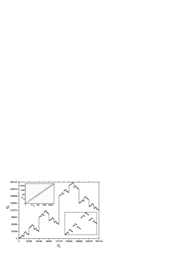
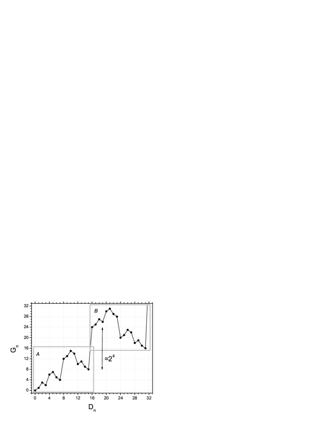
Figure 1: Self-similar Gray code curve

Figure 2: Self-similar construction of the Gray code curve

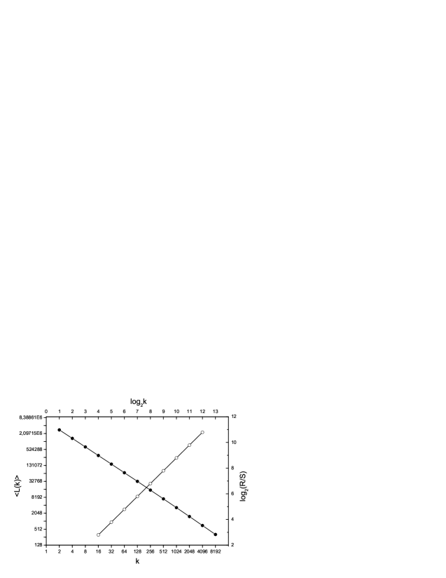
Figure 3: Histogram of the increments $\{|\Delta_{n}|\}$ in $\log_{2}-\log_{2}$ scale

Figure 4: Determination of the fractal dimension (left scale, solid dots) and Hurst exponent (right scale, circles)

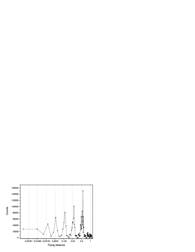
Figure 5: 2D trajectory for the Gray curve and zoom of the marked area

Figure 6: Histogram of Flying Distances in the random IFS Gray fractal with $N=22$ and bin size $0.02$

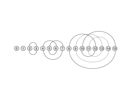
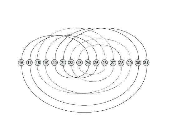
Figure 7: Orbits for Gray permutation of elements $0$ to $31$

Figure 8: Statistic of cycles as a function of $N$

References

- [1] Barnsley M 1988 Fractals everywhere Academic Press
- [2] Conder M 1999 Explicit definition of the binary reflected Gray code Discrete Mathematics 195 245–249
- [3] Conway J H, Sloane N J A and Wilks A R 1989 Gray codes for reflection groups Graphics and Combinatorics 5 315-325
- [4] Diakonos F K, Schmelcher P and Biham O 1998 Systematic computation of the least unstable periodic orbits in chaotic attractors Phys. Rev. Lett.81 4349–4352
- [5] Feder J 1988 Fractals Plenum Press NY
- [6] Forrester P J 2001 Random walks and random permutations J. Phys. A: Math. Gen.34 L517–23
- [7] Gardner M 1972 The curious properties of the Gray code and how it can be used to solve puzzles Sci. Amer. 227(2) 106–109
- [8] Gilbert W 1984 A cube-filling Hilbert curve Math. Intell. 6 78
- [9] Goddyn L, Gvozdjak P 2003 Binary Gray codes with long bit runs Electron. J. Combin. 10 R27, 1-10
- [10] Gray F 1953 Pulse Code Communication U. S. Patent 2 632 058, March 17
- [11] Higuchi T 1988 Approach to an irregular time series on the basis of the fractal theory Physica D 31 277–283
- [12] Hollstien R B 1971 Artificial Genetic Adaptation in Computer Control Systems (PhD thesis), University of Michigan
- [13] Hurst H E 1951 Long-term storage capacity of reservoirs Trans Am Soc Civ Engs 116 770–808
- [14] Knuth D E 2004 Generating all n-tuples. The Art of Computer Programming, Volume 4A: Enumeration and Backtracking, pre-fascicle 2A, http://www-cs-faculty.stanford.edu/ knuth/fasc2a.ps.gz
- [15] Knuth D E 2004 Generating all permutations. The Art of Computer Programming, Volume 4A: Enumeration and Backtracking, pre-fascicle 2B, http://www-cs-faculty.stanford.edu/ knuth/fasc2b.ps.gz
- [16] Krauth W and Opper M 1989 Critical storage capacity of the neural network J. Phys. A: Math. Gen.22 L519–23
- [17] Losee R M 2002 Optimal user-centered knowledge organization and classification systems: using non-reflected Gray codes, Journal of Digital Information http://jodi.tamu.edu/Articles/v02/i03/Losee/
- [18] Oshanin G and Voituriez R 2004 Random walk generated by random permutations of J. Phys. A: Math. Gen.37 6221–41
- [19] Pellett D E, Erwin J, Faulkner D, Ko W, Lander RL and Yager PM 1974 A Gray code hodoscope and fast beam particle tagging Nucl Instr & Meth 115 135–9
- [20] Press W H, Teukolsky S A, Vetterling W T, and Flannery B P 1997 Numerical Recipes in Fortran: The Art of Scienfic Computing Cambridge University Press
- [21] Rowe J, Whitley D, Barbulescu L and Watson JP 2004 Properties of Gray and binary representations Evolutionary Computation 12 47–76
- [22] Savage C 1997 A survey of combinatorial Gray codes SIAM Rev 39 605-629
- [23] Silverman J, Vickers V and E Sampson J L 1983 Statistical estimates of the n-bit Gray codes by restricted random generation of permutations of to IEEE Trans. Inf. Theory 29 894-901
- [24] Sloane NJA in On-line Encyclopedia of Integer Sequences, http://www.research.att.com/ njas/sequences/
- [25] Vartiainen J J, Möttönen M and Salomaa MM 2004 Efficient decomposition of quantum gates Phys. Rev. Lett.92 177902-1–4
- [26] White A 1987 Ringing the cosets Amer. Math. Monthly 94 721–746