The efficient computation of transition state resonances and reaction rates from a quantum normal form

Abstract

A quantum version of a recent formulation of transition state theory in phase space is presented. The theory developed provides an algorithm to compute quantum reaction rates and the associated Gamov-Siegert resonances with very high accuracy. The algorithm is especially efficient for multi-degree-of-freedom systems where other approaches are no longer feasible.

Introduction.— The question of how, as Marcus Marcus (1992) formulates it, a system “skis the reaction slope” is one of the crucial questions in reaction dynamics. Experimental techniques like photodissociation of jet-cooled molecules, molecular beam experiments or transition state spectroscopy give detailed information about the reaction process as has recently been demonstrated, e.g., for the ‘paradigm’ reaction of Hydrogen atom-diatom collisions (see, e.g., the review paper Skodje and Yang (2004)). A chemical reaction can often be viewed as the scattering problem across a saddle point of the interaction potential. The cumulative reaction probability is then given by

$$N(E)=\mbox{tr }\widehat{t}\,\widehat{t}^{T}=\sum_{n_{R}\,n_{P}}|\langle\psi_{\text{out}\,n_{p}}|\widehat{S}|\psi_{\text{in}\,n_{r}}\rangle|^{2}$$ (1)

where $\widehat{t}$ is the transmission subblock of the scattering operator $\widehat{S}$ for energy $E$ and the summation in the latter expression runs over all incoming reactant states with quantum numbers $n_{r}$ and outgoing product states with quantum numbers $n_{p}$. The ab initio quantum mechanical computation of $N(E)$ soon becomes very expensive if the number of atoms in the system increases beyond 3 and one has to resort to suitable approximations. The main approach to compute $N(E)$ classically is transition state theory which was invented by Eyring, Polanyi and Wigner in the 30’s. The main idea is to define a dividing surface that divides the energy surface into a reactant and a product component and compute the rate from the directional phase space flux through this surface. In order not to overestimate the rate the dividing surface must not be recrossed by reactive trajectories. In the 70’s Pechukas, Pollak and others Pechukas and McLafferty (1973) showed that for two degrees of freedom such a dividing surface can be constructed from a periodic orbit that leads to the so called periodic orbit dividing surface. Recently it has been shown that a generalization to higher dimension can be achieved from a normally hyperbolic invariant manifold (NHIM) Wiggins (1990) — a fundamentally new object that takes the place of the periodic orbit. The dynamics is controlled by the NHIM’s stable and unstable manifolds which act as separatrices that divide the reactive trajectories from the nonreactive trajectories. The NHIM, its stable and unstable manifolds and a dividing surface with the desired properties can be directly constructed from an algorithm based on a Poincaré-Birkhoff normal form procedure Uzer et al. (2001).

Much effort has been devoted to developing a quantum version of transition state theory whose implementation remains feasible for multi-dimensional systems (see the flux-flux autocorrelation function formalism by Miller and coworkers Miller (1998)). In this Letter we present a quantum version of the normal form procedure that lead to the construction of the high-dimensional phase space structures that govern the classical reaction dynamics and demonstrate that this quantum normal form approach to transition state theory provides an efficient procedure to compute quantum reaction rates and the corresponding Gamov-Siegert resonances Friedman and Truhlar (1991).

The quantum normal form.— The main idea of which the seed can already be found, e.g., in Hernandez and Miller (1993), is to derive a local approximation of the Hamilton operator of the scattering problem that is valid near the saddle, and in order to facilitate further computations, takes a much simpler form than the original Hamiltonian. This can be achieved in a systematic way by a procedure based on the Wigner-Weyl calculus that has been used by others before to compute energy spectra associated with stable equilibria Fried and Ezra (1988). Here the manipulations of an operator $\widehat{A}$ are expressed in terms of its symbol which is the function $A(p,x)$ on the $f$-degrees-of-freedom phase space $(p,x)\in\mathds{R}^{2f}$ defined by

$$\widehat{A}\psi(x)=\frac{1}{(2\pi\hbar)^{f}}\int_{\mathds{R}^{2f}}\mathrm{e}^{\frac{\mathrm{i}}{\hbar}\langle x-y,p\rangle}A\bigg{(}p,\frac{x+y}{2}\bigg{)}\,\psi(y)\,\mathrm{d}y\mathrm{d}p\,.$$ (2)

Defining the multiplication $*$ of two symbols $A$ and $B$ according to

$$A*B=A\exp\bigg{(}\mathrm{i}\frac{\hbar}{2}[\langle\stackrel{{\scriptstyle\leftharpoonup}}{{\partial}}_{x},\stackrel{{\scriptstyle\rightharpoonup}}{{\partial}}_{p}\rangle-\langle\stackrel{{\scriptstyle\rightharpoonup}}{{\partial}}_{x},\stackrel{{\scriptstyle\leftharpoonup}}{{\partial}}_{p}\rangle]\bigg{)}B\,,$$ (3)

where the arrows indicate whether the partial differentiation acts to the left (on $A$) or to the right (on $B$), gives the property that the quantization of the product of two symbols $A$ and $B$ is equal to the product of the quantizations of the individual symbols, i.e. $\widehat{A}\widehat{B}=\widehat{A*B}$ . The $*$-product leads to the definition of the Moyal bracket

$$\{A,B\}_{M}=\frac{\mathrm{i}}{\hbar}(A*B-B*A)\,.$$ (4)

We define the order $s$ of a monomial $p^{\alpha}x^{\beta}\hbar^{n}\equiv p_{1}^{\alpha_{1}}\cdots p_{f}^{\alpha_{f}}x_{1}^{\beta_{1}}\cdots x_{f}^{\beta_{f}}\hbar^{n}$ according to $s=\lvert\alpha\rvert+\lvert\beta\rvert+2n\equiv\alpha_{1}+\dots+\alpha_{f}+\beta_{1}+\dots+\beta_{f}+2n$, and denote the vector space of polynomials spanned by monomials of order $s$ by ${\mathcal{W}}^{s}$. For $A\in{\mathcal{W}}^{s}$ and $B\in{\mathcal{W}}^{s^{\prime}}$ we define the Moyal adjoint by $\operatorname{Mad}_{A}B:=\{A,B\}_{M}$, then its iterates satisfy $[\operatorname{Mad}_{A}]^{n}B\in{\mathcal{W}}^{n(s-2)+s^{\prime}}$.

We start from a Hamilton operator $\widehat{H}$ whose symbol has expansion

$$H=E_{0}+\sum_{s=2}^{\infty}H_{s}$$ (5)

where $E_{0}$ is a constant energy and $H_{s}\in{\mathcal{W}}^{s}$. Like in the case of classical transition state theory Uzer et al. (2001) we assume that the second order term is of the form

$$H_{2}=\lambda I+\omega_{2}J_{2}+\dots+\omega_{f}J_{f}$$ (6)

with the integrals

$$I=p_{1}x_{1}\,,\quad J_{k}=\frac{1}{2}\big{(}p_{k}^{2}+x_{k}^{2}\big{)}\,,\quad k=2,\dots,f\,.$$ (7)

This corresponds to a classical equilibrium point of saddle-center-$\dots$-center stability type (‘saddle’ for short), i.e. the matrix associated with the linearized system has one pair of real eigenvalues $\pm\lambda$ associated with the saddle or ‘reaction coordinate’ and $f-1$ pairs of imaginary eigenvalues $\pm\mathrm{i}\omega_{k}$, $k=2,\dots,f$, associated with the center or ‘bath’ degrees of freedom. Note that $p_{1}x_{1}=(\tilde{p}_{1}^{2}-\tilde{q}_{1}^{2})/2$ where $(p_{1},x_{1})$ and $(\tilde{p}_{1},\tilde{q}_{1})$ are related by a rotation of 45^∘. We restrict ourselves to the generic non-resonant case where the frequencies $\omega_{k}$, $k=2,\dots,f$, are rationally independent

In order to simplify the Hamiltonian $\widehat{H}$ we will transform it by successive conjugations with unitary operators, $\widehat{H}=:\widehat{H}^{(2)}\to\widehat{H}^{(3)}\to\widehat{H}^{(4)}\to\cdots\to\widehat{H}^{(N)}$, where

$$\widehat{H}^{(n)}=\mathrm{e}^{\mathrm{i}\widehat{W}_{n}/\hbar}\widehat{H}^{(n-1)}\mathrm{e}^{-\mathrm{i}\widehat{W}_{n}/\hbar}\,\,,$$ (8)

with $W_{n}\in{\mathcal{W}}^{n}$. Using the Moyal adjoint the symbol of the right hand side can be expanded as

$$H^{(n)}=\sum_{k=0}^{\infty}\frac{1}{k!}[\operatorname{Mad}_{W_{n}}]^{k}H^{(n-1)}\,\,.$$ (9)

If we expand furthermore each of the symbols $H^{(n)}$ in a generalized Taylor series as in (5), $H^{(n)}=E_{0}+\sum_{s\geq 2}H_{s}^{(n)}$, with $H_{s}^{(n)}\in W^{s}$, then using (9) the terms in these series can be related by

$$H_{s}^{(n)}=\sum_{k=0}^{[\frac{s-2}{k-2}]}\frac{1}{k!}[\operatorname{Mad}_{W_{n}}]^{k}H^{(n-1)}_{s-n(k-2)}\,\,,$$ (10)

where $[\cdot]$ denotes the integer part. Notice that for $s<n$, $H_{s}^{(n)}=H_{s}^{(n-1)}$, and for $s=n$ we obtain

$$H_{n}^{(n)}=H_{n}^{(n-1)}+\{W_{n},H_{2}\}$$ (11)

where we have used that $H^{(n)}_{2}=H_{2}$ for all $n\geq 3$ and that the Moyal bracket reduces to the Poisson bracket $\{\cdot,\cdot\}$ if one of the functions is quadratic. This is the homological equation which is familiar from the classical normal form algorithm, Uzer et al. (2001), and under the non-resonance conditions on the frequencies $\omega_{k}$, given any $H_{n}^{(n-1)}\in{\mathcal{W}}^{n}$ there exists a unique $W_{n}\in{\mathcal{W}}^{n}$ such that $H_{n}^{(n)}$ can be written as a function of the actions $I,J_{2},\cdots,J_{f}$ alone (or, equivalently, $H_{n}^{(n)}$ satisfies $\{I,H_{n}^{(n)}\}=\{J_{2},H_{n}^{(n)}\}=\cdots=\{J_{f},H_{n}^{(n)}\}=0$).

Choosing the generators of the unitary transformations $W_{n}$ recursively for $n=3,4,\ldots N$ as solutions of (11) we obtain an operator $\widehat{H}^{(N)}$ whose symbol is of the form $H^{(N)}=E_{0}+\sum_{s=2}^{N}H_{s}^{(N)}+R^{(N+1)}$ where the first part is a polynomial in the actions $I,J_{2},\cdots J_{f}$, i.e., is in normal form, and the remainder $R^{(N+1)}$ consists of terms of order $N+1$ and higher. In a final step we want to express the quantization of the normal form part as an operator function of the quantized actions $\hat{I}$ and $\widehat{J}_{k}$. To this end we use a recursion relation for $\widehat{I^{n}}$ (and a similar one for the $J_{k}$), $\widehat{I^{n+1}}=\widehat{I}\widehat{I^{n}}-\widehat{I^{n-1}}n^{2}\hbar^{2}/4$, which can be derived from the product formula (3). This allows us to express quantizations of powers of $I$ as a polynomial in powers of $\widehat{I}$. In this way we find a polynomial $H^{(N)}_{\text{QNF}}$ such that

$$U_{N}^{*}\widehat{H}U_{N}=H^{(N)}_{\text{QNF}}(\widehat{I},\widehat{J}_{2},\cdots,\widehat{J}_{f})+\widehat{R}^{(N+1)}\,\,,$$ (12)

where $U_{N}=\prod_{n=3}^{N}\mathrm{e}^{-\mathrm{i}\widehat{W}_{n}/\hbar}$. $H^{(N)}_{\text{QNF}}(\widehat{I},\widehat{J}_{2},\cdots,\widehat{J}_{f})$ is called the quantum normal form (QNF) of $\widehat{H}$ of order $N$. The remainder term $\widehat{R}^{(N+1)}$ has a symbol which is of order $N+1$ and is therefore very small near the saddle point. Hence the dynamics near the saddle point can be described with high accuracy by the QNF Hamiltonian. The advantage of the QNF Hamiltonian is that it is an operator function of the commuting operators $\widehat{I}$ and $\widehat{J}_{k}$ whose properties are well understood. Finally we point out that in the limit $\hbar\to 0$ we recover the classical normal form of order $N$, $\lim_{\hbar\to 0}H^{(N)}_{\text{QNF}}(I,J_{2},\cdots,J_{f})=H^{(N)}_{\text{cl}}$.

We implemented the algorithm of the QNF computation in the programming language C++.

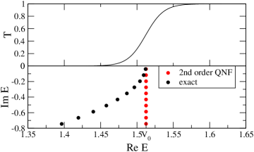
Figure 1: Transmission probability $T(E)$ and Gamov-Siegert resonances in the complex energy plane for the Eckart potential. The parameters are $a=1$, $10\,A=B=5$ for the Eckart potential, and $m=1$ and $\hbar=0.1$.

Resonances and reaction rates.— The eigenfunctions of the truncated QNF Hamiltonian are tensor products of harmonic oscillator wave functions for the center degrees of freedom $x_{k}$, $k=2,\dots,f$, and eigenfunctions of the operator

$$\widehat{I}=\frac{\hbar}{\mathrm{i}}\bigg{(}x_{1}\partial_{x_{1}}+\frac{1}{2}\bigg{)}$$ (13)

associated with the saddle direction. The operator $\widehat{I}$ has eigenfunctions Colin de Verdière and Parisse (1994a)

$$\psi_{\text{out}\,\pm}(x_{1})=\Theta(\pm x_{1})\lvert x_{1}\rvert^{-1/2+\mathrm{i}I/\hbar}\,\,,$$ (14)

$\Theta$ being the step function, which are outgoing waves. Incoming waves can be defined from the Fourier transforms

$$\begin{split}\psi_{\text{in}\,\pm}(x_{1})=\frac{1}{\sqrt{2\pi\hbar}}\int{\psi}_{\text{out}\,\mp}^{*}(y_{1})\mathrm{e}^{\frac{\mathrm{i}}{\hbar}x_{1}y_{1}}\,\,\mathrm{d}y_{1}\,.\end{split}$$ (15)

Note that in order to classify the eigenfunctions as ‘outgoing’ or ‘incoming’ it is convenient to rotate the coordinates $(p_{1},x_{1})$ back to the more standard notation $(\tilde{p}_{1},\tilde{q}_{1})$ for a potential barrier mentioned above. Expressing the functions $\psi_{\text{in}\,\pm}$ in terms of $\psi_{\text{out}\,\pm}$ gives the entries of a ‘local S-matrix’,

$$\psi_{\text{in}\,+} = S_{n\,11}\,\psi_{\text{out}\,+}+S_{n\,12}\,\psi_{\text{out}\,-}\,,$$ (16)

$$\psi_{\text{in}\,-} = S_{n\,21}\,\psi_{\text{out}\,+}+S_{n\,22}\,\psi_{\text{out}\,-}\,.$$ (17)

Here $n$ denotes the vector of nonnegative integers $(n_{2},\dots,n_{f})$ formed by the quantum numbers of the modes in the center directions. The local S-matrix is block diagonal due to the separability of the QNF. Mode mixing is a ‘global’ effect which occurs from connecting the local wave functions to the asymptotic reactants and products wave functions. However, the local S-matrix alone already contains the full information needed to compute reaction rates and resonances.

Evaluating the integrals (15) gives

$$S_{n}(E)=\frac{\mathrm{e}^{\mathrm{i}(\frac{\pi}{4}-\frac{I}{\hbar}\ln\hbar)}}{\sqrt{2\pi}}\Gamma\bigg{(}\frac{1}{2}-\mathrm{i}\frac{I}{\hbar}\bigg{)}\begin{pmatrix}-\mathrm{i}\mathrm{e}^{-\frac{\pi}{2}\frac{I}{\hbar}}&\mathrm{e}^{\frac{\pi}{2}\frac{I}{\hbar}}\\ \mathrm{e}^{\frac{\pi}{2}\frac{I}{\hbar}}&-\mathrm{i}\mathrm{e}^{-\frac{\pi}{2}\frac{I}{\hbar}}\end{pmatrix}$$ (18)

with $I$ being implicitly defined by

$$H^{(N)}_{\text{QNF}}\big{(}I,\hbar(n_{2}+1/2),\dots,\hbar(n_{f}+1/2)\big{)}=E\,.$$ (19)

The transmission probability of mode $n$ is

$$T_{n}(E)=\lvert S_{n\,12}(E)\rvert^{2}=(1+\mathrm{e}^{-2\pi\frac{I}{\hbar}})^{-1}\,,$$ (20)

which gives the cumulative reaction probability $N(E)=\sum_{n}T_{n}(E)$. The S-matrix has poles at $I=-\mathrm{i}\hbar(n_{1}+1/2)$ for nonnegative integers $n_{1}$ and these define the Gamov-Siegert resonances via (19).

Examples.— We at first illustrate the procedure for 1D potential barriers, i.e. Hamiltonians of the form $H=p^{2}/(2m)+V(x)\,,$ where $V(x)$ has a maximum which we can assume to be at $x=0$. The second order QNF is easily obtained and gives the well know result $\widehat{H}_{\text{QNF},\,2}=V(0)+\lambda\widehat{I}$ with $\lambda=(-V^{\prime\prime}(0)/m)^{1/2}$ which is equivalent to approximating the potential barrier by an inverted parabola. The first nontrivial correction to this result comes from the fourth order QNF $\widehat{H}_{\text{QNF},\,4}$ given by

$$\begin{split}&V(0)+\lambda\widehat{I}+\frac{1}{16m^{2}\lambda^{2}}\left(\frac{5}{3m\lambda^{2}}V^{\prime\prime\prime}(0)+V^{IV}(0)\right)\widehat{I}^{2}\\ &-\frac{1}{64m^{2}\lambda^{2}}\left(\frac{7}{9m\lambda^{2}}V^{\prime\prime\prime}(0)+V^{IV}(0)\right)\hbar^{2}\,.\end{split}$$ (21)

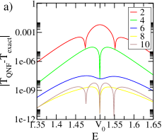
Figure 2: (a) Errors for the transmission probability of the Eckart potential computed from the QNF. (b) Errors for the QNF resonances (differences between the corresponding QNF and exact complex energies) of the Eckart potential as a function of the quantum number $n_{1}$. The different colors correspond to different orders of the QNF. The parameters for the Eckart potential are the same as in Fig. 1.

We apply the QNF to the Eckart potential Eckart (1930)

$$V_{\text{Eckart}}(x)=A\frac{\mathrm{e}^{(x+x_{0})/a}}{1+\mathrm{e}^{(x+x_{0})/a}}+B\frac{\mathrm{e}^{(x+x_{0})/a}}{(1+\mathrm{e}^{(x+x_{0})/a})^{2}}$$ (22)

with $x_{0}=a\ln(B+A)/(B-A)$ and $B>A\geq 0$. Figure 1 shows the exact transmission probability which is known analytically, and the exact string of resonances together with the resonances from the second order QNF which have constant imaginary part. The bending of the string of exact resonances is a nonlinear effect that is very well described already by the fourth order QNF. The excellent accuracy of the resonances and the cumulative reaction probability computed from higher orders of the QNF is illustrated in Fig. 2.

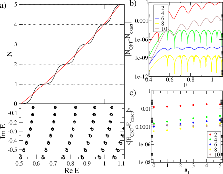
Figure 3: (a) The top panel shows the cumulative reaction probability $N(E)$ (oscillatory curve) and the classical flux divided by $2\pi\hbar$ (smooth curve) for the Eckart-Morse potential defined in the text with $\epsilon=0$. The bottom panel shows the resonances in the complex energy plane marked by circles for the uncoupled case $\epsilon=0$ and by crosses for the strongly coupled case $\epsilon=0.3$. For the coupled case the numerically exact resonances are computed from the complex dilation method Moiseyev (1998). The parameters for the Eckart potential are the same as in Fig. 1. The parameters for the Morse potential are $D_{e}=1$ $\alpha=1$. Again we choose $m=1$ and $\hbar=0.1$. (b) Errors for the cumulative reaction probability in (a) for different orders of the QNF. (c) Average errors $<|E_{\text{QNF}}-E_{\text{exact}}|>_{n_{1}}=\sum_{n_{2}=0}^{5}|E_{\text{QNF}}(n_{1},n_{2})-E_{\text{exact}}(n_{1},n_{2})|/6$ for the QNF resonances in (a) for the coupled case $\epsilon=0.3$ as a function of the quantum numbers $n_{1}$.

We next consider the two-degree-of-freedom example of a Hamiltonian with an Eckart potential in the $x_{1}$-direction, a Morse potential

$$V_{\text{Morse}}(x_{2})=D_{e}\left(\mathrm{e}^{-2\alpha x_{2}}-2\mathrm{e}^{-\alpha x_{2}}\right)$$ (23)

in the $x_{2}$-direction, plus a kinetic coupling $\epsilon p_{1}p_{2}$. In Fig. 3 the cumulative reaction probability and the resonances computed from the QNF are compared with the exact results. In the uncoupled case $\epsilon=0$, $N(E)$ increases as a function of $E$ at integer steps each time a new transition channel opens, i.e. when the transmission probability $T_{n_{2}}(E)$ of a Morse oscillator mode $n_{2}$ switches from 0 to 1. For both the uncoupled and strongly coupled case the resonances form a distorted lattice parametrized by the mode quantum number $n_{2}$ in horizontal direction and the quantum number $n_{1}$ in vertical direction. Similar to the 1D example, each string of constant $n_{2}$ is related to one step of $N(E)$.

Like in the 1D case the agreement of the QNF results with the exact results is excellent and this remains the case even for the strongly coupled system. The QNF is an asymptotic expansion which in general does not converge. For the system shown in the example this can be seen from the fact that the 10th order QNF does not lead to an improvement of the results obtained from the 8th order QNF.

Conclusions.— The QNF computation of reaction probabilities and the corresponding Gamov-Siegert resonances is highly promising since it opens the way to study high dimensional systems for which other techniques based on the ab initio solution of the quantum scattering problem like the complex dilation method Moiseyev (1998) or the utilization of an absorbing potential Neumaier and Mandelshtam (2001) are no longer feasible. In fact, the numerical effort for computing the QNF is only slightly higher than the effort for computing the classical normal form (NF). The main difference is that the Poisson bracket in the classical NF needs to be replaced by the Moyal bracket. The storage of the QNF polynomials also requires only a disk space similar to the classical NF. Moreover, the QNF gives an explicit formula for the resonances from which they can be computed directly by inserting the corresponding quantum numbers. This leads to a direct assignment of the resonances. The QNF provides a quantum version of transition state theory that, in the semiclassical limit, is in accord with the classical phase structures that govern the reaction dynamics. In fact, the classical phase space structures form the skeleton for the scattering and resonance wavefunctions, and exploiting this relationship which will give a deep insight into the now experimentally accessible quantum reaction dynamics is the subject of our future studies (see also Creagh (2004)).

This work was supported by the Office of Naval Research, EPSRC and the Royal Society.

References

- Marcus (1992) R. A. Marcus, Science 256, 1523 (1992).
- Skodje and Yang (2004) R. T. Skodje and X. Yang, Int. Rev. Phys. Chem. 23, 253 (2004).
- Pechukas and McLafferty (1973) P. Pechukas and F. J. McLafferty, J. Chem. Phys. 58, 1622 (1973); P. Pechukas and E. Pollak, J. Chem. Phys. 69, 1218 (1978).
- Wiggins (1990) S. Wiggins, Physica D 44, 471 (1990); S. Wiggins, Normally Hyperbolic Invariant Manifolds in Dynamical Systems (Springer, Berlin, 1994); S. Wiggins, L. Wiesenfeld, C. Jaffé, and T. Uzer, Phys. Rev. Lett. 86, 5478 (2001).
- Uzer et al. (2001) T. Uzer, C. Jaffé, J. Palacián, P. Yanguas, and S. Wiggins, 957 (2001); H. Waalkens, A. Burbanks, and S. Wiggins, J. Chem. Phys. 121, 6207 (2004).
- Miller (1998) W. H. Miller, J. Phys. Chem. A 102, 793 (1998).
- Friedman and Truhlar (1991) R. S. Friedman and D. G. Truhlar, Chem. Phys. Lett. 183, 539 (1991); T. Seideman and W. H. Miller, J. Chem. Phys. 95, 1768 (1991).
- Hernandez and Miller (1993) R. Hernandez and W. H. Miller, Chem. Phys. Lett. 214, 129 (1993); R. Hernandez, J. Chem. Phys. 101, 9534 (1994).
- Fried and Ezra (1988) L. E. Fried and G. S. Ezra, J. Chem. Phys. 92, 3144 (1988); P. Crehan, J. Phys. A 23, 5815 (1990).
- Colin de Verdière and Parisse (1994a) Y. Colin de Verdière and B. Parisse, Comm. PDE 19, 1535 (1994a); Ann. Inst. Henri Poincaré (Physique Théorique) 61, 347 (1994b); Comm. Math. Phys. 205, 459 (1999).
- Nonnenmacher and Voros (1997) S. Nonnenmacher and A. Voros, J. Phys. A:Math. Gen. 30, 295 (1997).
- Eckart (1930) C. Eckart, Phys. Rev. 35, 1303 (1930).
- Moiseyev (1998) N. Moiseyev, Phys. Rep. 302, 211 (1998); W. P. Reinhardt, Ann. Rev. Phys. Chem. 33, 223 (1982); B. Simon, Phys. Lett. A 71, 211 (1979).
- Neumaier and Mandelshtam (2001) A. Neumaier and V. A. Mandelshtam, Phys. Rev. Lett. 86, 5031 (2001).
- Creagh (2004) S. C. Creagh, Nonlinearity 17, 1261 (2004); ibid. 18, 2089 (2005)