On the attractors of two-dimensional Rayleigh oscillators including noise

Abstract

We study sustained oscillations in two-dimensional oscillator systems driven by Rayleigh-type negative friction. In particular we investigate the influence of mismatch of the two frequencies. Further we study the influence of external noise and nonlinearity of the conservative forces. Our consideration is restricted to the case that the driving is rather weak and that the forces show only weak deviations from radial symmetry. For this case we provide results for the attractors and the bifurcations of the system. We show that for rational relations of the frequencies the system develops several rotational excitations with right/left symmetry, corresponding to limit cycles in the four-dimensional phase space. The corresponding noisy distributions have the form of hoops or tires in the four-dimensional space. For irrational frequency relations, as well as for increasing strength of driving or noise the periodic excitations are replaced by chaotic oscillations.

I Introduction

The first comprehensive theory of nonlinear oscillations was developed by Lord Rayleigh in the years 1883–1894 and is represented in his pioneering book Rayleigh (1894). The present state of art of nonlinear dynamics was deeply influenced by the pioneering work of Leonid Shilnikov (see Shilnikov, 1997; Shilnikov et al., 1998a, b, and references therein) which is reflected e.g. in the books of Anishchenko (1995); Anishchenko et al. (2002). In the last decade many investigations were devoted to the stochastic dynamics of dissipative hamiltonian systems (Klimontovich, 1994; Anishchenko et al., 2002).

In this paper we extend previous studies on rotational excitations of two-dimensional oscillators driven by Rayleigh-type negative friction Erdmann et al. (2000, 2002). The study of driven oscillatory modes on a plane has interesting applications for modeling animal mobility all the way from microorganisms like bacteria and Dictyostelium discoedium slime mold (Czirók et al., 1996; Rappel et al., 1999; Ben-Jacob et al., 2000) upto flocks of birds (Toner and Tu, 1995; Weimerskirch et al., 2001), schools of fish (Parrish et al., 2002; Inada and Kawachi, 2002; Niwa, 1994; Hubbard et al., 2004), swarms of Daphnia (Ordemann et al., 2003; Erdmann et al., 2004) or wildebeest (Topaz and Bertozzi, 2004). For example we introduced in earlier work the general idea of stochastically moving species, active Brownian particles. We want to recall this approach which will be used later on. Active Brownian particles are Brownian particles with the ability to take up energy from the environment and use it for the acceleration of motion. Simple models composed of active Brownian particles were studied in many earlier works (e.g. Klimontovich, 1994; Schienbein and Gruler, 1993; Helbing and Molnár, 1995).

A specific problem we would like to address here is: what is the consequence of broken radial symmetry (asymmetry of the conservative forces). In particular we are interested in the problem: Can spontaneous rotations be stopped by certain amount of asymmetry? In contrast to previous studies Vicsek et al. (1995); Czirók et al. (1996); Albano (1996); Shimoyama et al. (1996); Czirók et al. (1997); Levine et al. (2001); Grégoire et al. (2001); Hubbard et al. (2004); Grégoire and Chaté (2004) the self-propelling feature is modeled here by active Brownian particles with negative friction Ebeling et al. (1999); Schweitzer et al. (1998); Erdmann et al. (2000); Steuernagel et al. (1994) which are able to convert stored internal energy into motion. In this paper, we will study only the motion, especially rotational ones, in external fields on a two-dimensional plane.

The article is organized as follows. In Section II we introduce the equations of motion, the pumping by negative friction and outline the basic dynamics of our model including Langevin equations. In Section III we outline our previous studies of rotationally symmetric external potentials and discuss the attractors for rational frequency relations. In Section IV we give an analysis of frequency mismatch and of Arnold-type bifurcations of linear oscillators as a function of the mismatch. Further we study in Section V the limit cycle attractors of nonlinear oscillators with radial symmetry. In Section VI we investigate the influence of noise on the attractors and show that noise leads to a broadening on the line-attractors.

II Dynamic equations for two-dimensional oscillators

The dynamics of the systems studied here is based on Langevin equations, known from the theory of conventional Brownian motion (Langevin, 1908; Hänggi et al., 1990). For the two-dimensional space we get four first order coupled differential equations in the phase space $\{x_{1},x_{2},v_{1},v_{2}\}$:

$$\dot{x}_{1} = v_{1}$$ (1a)

$$\dot{x}_{2} = v_{2}$$ (1b)

$$\dot{v}_{1} = \frac{1}{m}\frac{\partial U}{\partial x_{1}}-\gamma(v_{1},v_{2})v_{1}+\sqrt{2D}\xi_{1}(t)$$ (1c)

$$\dot{v}_{2} = \frac{1}{m}\frac{\partial U}{\partial x_{2}}-\gamma(v_{1},v_{2})v_{2}+\sqrt{2D}\xi_{2}(t)\,.$$ (1d)

In this dynamics we assumed three kinds of forces in the dynamics:

1. Conservative external forces generated by the potentials $U(x_{1},x_{2})$,

2. nonlinear dissipative forces modeled by the friction $(-\bm{v}\gamma(\bm{v}))$,

3. stochastic forces assigned by $\xi(t)$.

Several linear and nonlinear conservative forces will be introduced and studied in the following sections. The dissipative forces are modeled by the friction function $\gamma(\bm{v})$. This function is the source of dissipative interactions with the surrounding. In equilibrium the friction is passive

$$\gamma(\bm{v})=\gamma_{0}={\rm const.}$$ (2)

We will consider here in more detail active friction modeled by the classical Rayleigh law (Rayleigh, 1894):

$$\gamma(\bm{v})=\gamma(v_{1},v_{2})=\alpha-\beta(v_{1}^{2}+v_{2}^{2})\,.$$ (3)

The stochastic forces are modeled by white Gaussian noise $\xi$ with vanishing mean and

$$\langle\xi(t)\xi(t^{\prime})\rangle=\delta(t-t^{\prime})$$ (4)

and scaled with strength $D$. In equilibrium and in case of passive friction following Einstein (1956) one gets an energy balance between the strength of the stochastic force, $D$, and the passive friction acting on the object. It is expressed by the simple fluctuation-dissipation relation

$$D=\frac{\gamma_{0}\theta}{m}$$ (5)

where $\theta=k_{B}T$ is a measure for the temperature.

III Attractors for linear oscillators driven by Rayleigh friction

We will study in this section two-dimensional linear oscillators described by the potential

$$U(x_{1},x_{2})=\frac{m}{2}(\omega_{1}^{2}x_{1}^{2}+\omega_{2}^{2}x_{2}^{2})$$ (6)

which are driven by Rayleigh-type negative friction as in Eq. (3). It is well known since Rayleigh (1894) that in the one-dimensional case the system possesses a limit cycle corresponding to sustained oscillations with the energy $E_{0}=\alpha/\beta$. The two-dimensional case is much more complicated. Erdmann et al. (2000) have shown for the symmetrical case with $\omega_{2}=\omega_{1}$, that two limit cycles in the four-dimensional phase space are developed. The projection of these sustained oscillations on the $\{v_{1},v_{2}\}$-plane and on the $\{x_{1},x_{2}\}$-plane are circles

$$v_{1}^{2}+v_{2}^{2} =v_{0}^{2} =\frac{\alpha}{\beta}$$ (7a)

$$x_{1}^{2}+x_{2}^{2} =r_{0}^{2} =\frac{v_{0}}{\omega_{1}}$$ (7b)

The limit cycle energy is

$$E_{0}=\frac{mv_{0}^{2}}{2}+\frac{m\omega_{1}^{2}}{2}\,r_{0}^{2}\;.$$ (8)

Ebeling et al. (1999) have shown, that any initial value of the energy converges (at least in the limit of strong pumping) to

$$H\longrightarrow E_{0}=mv_{0}^{2}$$ (9)

This corresponds to an equal distribution between kinetic and potential energy i.e. both parts contribute the same amount to the total energy. The motion on the limit cycle in the four-dimensional space may be represented by the four equations

$$x_{1} = r_{0}\cos(\omega_{0}t+\phi_{0})$$ (10a)

$$v_{1} = -r_{0}\omega_{0}\,\sin(\omega_{0}t+\phi_{0})$$ (10b)

$$x_{2} = r_{0}\sin(\omega_{0}t+\phi_{0})$$ (10c)

$$v_{2} = r_{0}\omega_{0}\,\cos(\omega_{0}t+\phi_{0})$$ (10d)

The angular frequency follows by estimations of the time the particle needs for one period moving on the circle of radius $r_{0}$ with constant speed $v_{0}$:

$$\omega_{0}=\frac{v_{0}}{r_{0}}=\omega_{1}=\omega_{2}\;.$$ (11)

This means, the particle rotates even at strong pumping with the frequency given by the linear oscillator frequency $\omega_{1}=\omega_{2}$. The trajectory defined by Eqs. (10) is an exact solution of the dynamic equations describing the first (forward) limit cycle. The shape of the trajectory is like a hoop in the four-dimensional space. Most projections to the two-dimensional subspaces are circles or ellipses however there are two subspaces namely $\{x_{1},v_{2}\}$ and $\{x_{2},v_{1}\}$ where the projection is like a rod Erdmann et al. (2000). Reversing the initial velocities of the system, a second limit cycle can be obtained. This limit cycle forms also a hula hoop which is different from the first one. However both limit cycles have the same projections on the $\{x_{1},x_{2}\}$ and on the $\{v_{1},v_{2}\}$-plane. The projection to the $\{x_{1},x_{2}\}$-plane has the opposite sense of rotation in comparison with the first limit cycle. The projections of the two hoops on the $\{x_{1},x_{2}\}$-plane or on the $\{v_{1},v_{2}\}$-plane are two-dimensional rings. The hoops intersect perpendicular $\{x_{1},v_{2}\}$- and $\{x_{2},v_{1}\}$-planes. The projections to these planes are rod-like and the intersection manifold with these planes consists of two ellipses located in the diagonals of the planes (Erdmann et al., 2000).

So far we repeated known results for the symmetrical case. Dynamical systems with radial symmetry are degenerate and structurally unstable in the mathematical context. From the physical viewpoint, radial symmetry is a special situation, i.e. the gravitational field of point masses or the Coulomb field for charges has strict radial symmetry. Therefore radial symmetry holds also for a two-dimensional mass-point pendulum. In real physical systems the radial symmetry is in general broken, e.g. a real pendulum in the earth field has no strict radial symmetry. Thus the oscillator with radial symmetry can only be considered as a particular case of corresponding real system which often has some asymmetry. Thus our motivation is, to investigate the consequences of broken radial symmetry and deviations from linearity on the generation of oscillatory modes.

First we are going to study systems with frequency mismatch $\omega_{2}\neq\omega_{1}$. In the conservative case $\gamma=0$ and $D=0$ we find a dense set of exact solution for the deterministic dynamics given by

$$x_{1}(t) = A_{1}\cos(\omega_{1}t+\Phi_{1})$$ (12a)

$$v_{1}(t) = -A_{1}\omega_{1}\sin(\omega_{1}t+\Phi_{1}),$$ (12b)

$$x_{2}(t) = A_{2}\sin(\omega_{2}t+\Phi_{2})$$ (12c)

$$v_{2}(t) = A_{2}\omega_{2}\cos(\omega_{2}t+\Phi_{2})\,,$$ (12d)

where $A_{i}$ and $\Phi_{i}$ are given by the (arbitrary) initial conditions. Let us study now the driven case with negative friction according to the Rayleigh law (3) without noise. Then for $\alpha>0$ the above periodic solution (12) would remain to be a solution, if

$$v_{1}^{2}+v_{2}^{2}=v_{0}^{2}=\frac{\alpha}{\beta}$$ (13)

is fulfilled. In the case of symmetrical oscillators $\omega_{1}=\omega_{2}=\omega_{0}$ we could fulfill this condition in an exact way by a special choice of the amplitudes:

$$A_{1}=A_{2}=r_{0}=\frac{v_{0}}{\omega_{0}}$$ (14)

This means, we find instead of a dense set of exact solutions just one attracting solution (which still is exact). This periodic and stable exact solution represents a limit cycle corresponding to a circular path even at strong pumping with the frequency given by the simple harmonic oscillator frequency $\omega_{0}$. However in the case $\omega_{1}\neq\omega_{2}$ the situation is much more difficult than in the symmetrical case. First we are looking for approximate stable solutions in the case of rational relations of the frequencies $\omega_{2}=n\omega_{0}$ and $\omega_{1}=m\omega_{0}$ with $n,m=1,2,\ldots$. The condition (13) is in average over one period fulfilled, if

$$A_{1}^{2}\omega_{1}^{2}=A_{2}^{2}\omega_{2}^{2}=v_{0}^{2}$$ (15)

This way we get the stable amplitudes and phases

$$A_{1}=\frac{v_{0}}{\omega_{1}}\,;\qquad A_{2}=\frac{v_{0}}{\omega_{2}}$$ (16a)

$$\Phi_{1}=-\frac{\pi}{2}\,;\qquad\Phi_{2}=+\frac{\pi}{2}$$ (16b)

We will show that these approximative solutions describe at least for small relations $n:m$ again a pair of forward/backward limit cycles. By introducing the approximation 16 into Eq. (12) we find for the $n>m$ the following analytical approximation for the limit cycles:

$$x_{1}(t) = r_{0}\sin(m\omega_{0}t)$$ (17a)

$$v_{1}(t) = r_{0}m\omega_{0}\cos(m\omega_{0}t)$$ (17b)

$$x_{2}(t) = r_{0}\cos(n\omega_{0}t)$$ (17c)

$$v_{2}(t) = -r_{0}n\omega_{0}\sin(n\omega_{0}t)\,.$$ (17d)

The curves obtained by this approximation for $n:m=2,3,4,5$ are shown in Fig. 1.

Figure 1: Projections of asymmetric limit cycles to the $\{x_{1},x_{2}\}$-plane for several cases of rational relations between the two frequencies $m:n=2,3,4,5$ (analytical approximation for the attractors (Eqs. (12) and (16)).

In the analytical approximation given above, the forward limit cycles and the backward limit cycles have identical projections on the $\{x_{1},x_{2}\}$-plane. However our analytical formula (Eqs. (12) and (16)) is only a rough approximation, as we will demonstrate by simulations. We show in Figs. 2 and 3 the result of simulations for the two attractors in the case $m:n=2$.

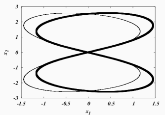
Figure 2: Projections of the two limit cycles to the $\{x_{1},x_{2}\}$-plane corresponding to $m:n=2$ resonance obtained from simulations (Rayleigh law: $\alpha=5$, $\beta=1$).

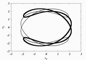
Figure 3: Projections of the two limit cycles to the $\{v_{1},v_{2}\}$-plane corresponding to $m:n=2$ to the $\{v_{1},v_{2}\}$-plane obtained from simulations (same parameters as in Fig. 2).

Clearly, the two attractors have different projections on the $\{x_{1},x_{2}\}$-plane (see Fig. 2) as well as on the $\{v_{1},v_{2}\}$-plane (see Fig. 3). As we see, the projection differ in amplitude and phase a little bit from the analytical approximation; in particular clockwise and counterclockwise limit cycles are shifted in the projections. It is interesting to note that the projections to the $\{x_{1},v_{1}\}$-plane and to the $\{x_{2},v_{2}\}$-plane shown in Fig. 4 are equal for the clockwise and the counterclockwise limit cycles.

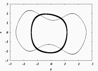
Figure 4: Projections of the two limit cycles to the $\{x_{2},v_{2}\}$-plane for $m:n=2$ and respectively obtained from simulations (same parameters as in Fig. 2). Clockwise and counterclockwise limit cycle have practically the same projections.

The rather complex winding structure of the attractor for $n=2$ in the four-dimensional phase space can be guessed by looking at projections on three-dimensional subspaces as demonstrated in Fig. 5.

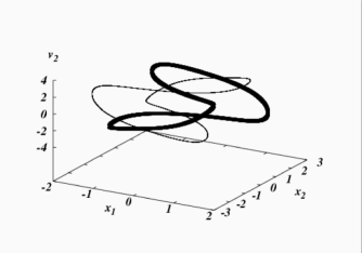
Figure 5: Projections of the two limit cycles to the $\{x_{1},x_{2},v_{2}\}$-plane corresponding to the $m:n=2$-resonance obtained from simulations (same parameters as in Fig. 2).

The results obtained from simulations for $n=3$ are shown in Figs. 6 and 7. We see that the attractors obtained from simulations are more complex than the from the nice and rather symmetrical curves obtained from the analytical approximation for the case $n=3$ which were presented in Fig. 1. With increasing rational $n$ the attractor fills more or less dense a rectangular region. For irrational values of $\omega_{2}/\omega_{1}$ the trajectories are always dense in a nearly rectangular region of the coordinate space. This case will be studied below.

Figure 6: Projections of the two limit cycles to the $\{x_{1},x_{2}\}$-plane corresponding to the $m:n=3$-resonance obtained from simulations ($\omega_{1}=2.7$, $\omega_{2}=1$, all other parameters as in Fig. 2).

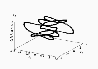
Figure 7: Projections of the two limit cycles for $m:n=3$ to the $\{x_{1},x_{2},v_{2}\}$-plane obtained from simulations.

IV Bifurcation analysis of the linear oscillators with frequency mismatch

Our study was limited so far to small rational frequency relations $m:n$ and small or moderate strength of driving (small positive values of the bifurcation parameter $\alpha$). In order to introduce the consequences of a an irrational frequency mismatch between the partial subsystems in a more general setting we write the expression for the potential Eq. (6) as follows:

$$U(x_{1},x_{2}) = \frac{m}{2}\,\omega_{0}^{2}(x_{1}^{2}+\Delta^{2}x_{2}^{2}),$$ (18a)

$$\Delta = \frac{\omega_{1}}{\omega_{2}};\qquad\omega_{0}=\omega_{1}.$$ (18b)

In the general case the potential $U(x_{1},x_{2})$ has an elliptic, slightly extended shape, the asymmetry is measured by the parameter $\Delta$. For irrational values of $\Delta$ the solutions in the conservative case $\alpha=\beta=0$ fill densely a box in the phase space. In the general driven case the deterministic part of Eq. (1) may be written as

$$\dot{x}_{1} = v_{1}$$ (19a)

$$\dot{v}_{1} = \left[\alpha-\beta\left(v_{1}^{2}+v_{2}^{2}\right)\right]v_{1}-\omega_{0}^{2}x_{1}$$ (19b)

$$\dot{x}_{2} = v_{2}$$ (19c)

$$\dot{v}_{2} = \left[\alpha-\beta\left(v_{1}^{2}+v_{2}^{2}\right)\right]v_{2}-\omega_{0}^{2}\Delta^{2}x_{2}$$ (19d)

The system (19) is structurally stable or is one of the common propositions according to V. I. Arnold’s nomenclature (Arnold, 1965). It can be interpreted as a model for one oscillator on the plane or as a model for two interacting linear oscillators.

To understand the dynamics of system (19) in the general case, we introduce a complex variable $z=x_{1}+jx_{2}$. Let us first turn again to the symmetric case where $\omega_{1}=\omega_{2}=\omega_{0}$. Then from (19) follows

$$\ddot{z}-\beta\left(\frac{\alpha}{\beta}-|\dot{z}|^{2}\right)\dot{z}+\omega_{0}^{2}z=0.$$ (20)

Equation (20) has periodic solutions of the form:

$$z(t)=z\exp(\pm j\omega_{0}t)=|z|\exp(j\Phi)\,\exp(\pm j\omega_{0}t),$$ (21)

where the phase $\Phi$ takes any value in the interval $[0,2\pi]$. When we consider the symmetric case, we have an infinite number of periodic solutions (see Eq. (21)). However, linear analysis cannot yield information about their stability. In numeric calculations, we can detect several limit cycles each of them possessing its own type of symmetry. As by Erdmann et al. (2002) has been investigated, the stability of periodic solutions can can be predicted by the calculation of the Floquet multipliers of the fixed points within the Poincarè section of the limit cycle. When there is a detuning ($\Delta\neq 1$), only two limit cycles, representing clockwise and counterclockwise rotations remain stable as has already been found by Erdmann et al. (2000). All other solutions have at least one multiplier leaving the unit circle on the complex plane. The two limit cycles representing the rotations of a particle in the coordinate space are situated within the first Arnold tongue whereas outside this region the existence of the cycles vanishes and the particles move irregularly. Increasing the detuning $\Delta$ any further new stability regions appear which represent the period-$n$ cycles of the oscillators as have been shown in Figs. 1-7. The parameter region where stability of periodic motion can be observed is shown in Fig. 8.

Figure 8: Stability regions (Arnold tongues) of the $m:n$ resonances. Within the light gray areas the limit cycles as described above are stable. The arrows show the parameter set of Figs. 2-7.

V Nonlinear oscillators with radial symmetry

In the present section we will discuss several extensions of the theory developed in the previous section to nonlinear oscillators. However, for simplicity, we will restrict our study to systems with rotational symmetry, $U=U(r)$ with $U(0)=0$ and $U(r)-$ monotonically increasing. For the general case of radially symmetric but anharmonic potentials $U(r)$ the equal distribution between potential and kinetic energy is violated. In other words the relation $mv_{0}^{2}=m\omega_{0}^{2}r_{0}^{2}$ which leads to $\omega_{0}=v_{0}/r_{0}=\omega$ is no more valid. This relation has to be replaced by the more general condition that on the limit cycle the attracting radial forces are in equilibrium with the centrifugal forces. This leads to

$$\frac{mv_{0}^{2}}{r_{0}}=|U^{\prime}(r_{0})|$$ (22)

If $v_{0}$ is given, the equilibrium radius may be found from the implicit relation

$$v_{0}^{2}=\frac{r_{0}}{m}|U^{\prime}(r_{0})|$$ (23)

Then the frequency of the limit cycle oscillations is given by

$$\omega_{0}^{2}=\frac{v_{0}^{2}}{r_{0}^{2}}=\frac{|U^{\prime}(r_{0})|}{mr_{0}}$$ (24)

In the case of linear oscillators this leads us back to previous result given in Sec. III. For the case of quartic oscillators

$$U(r)=\frac{k}{4}r^{4}$$ (25)

we get the limit cycle frequency

$$\omega_{0}=\frac{k^{1/4}}{v_{0}^{1/2}}$$ (26)

The explicite solution (10) remains valid, i.e. we find again an exact analytical description of the pair of limit cycles. For monotonically increasing potentials there exist just one stable radius $r_{0}$. If the equation (23) has several solutions, the dynamics might be much more complicated. An interesting application of the theoretical results given above is the case of Coulomb forces Schimansky-Geier et al. (2005). Another possible application is the following: Let us imagine a system of Brownian particles which are pairwise bound by a Lennard-Jones-like potential $U(|r_{1}-r_{2}|)$ to dumb-bell-like configurations. Then the motion consists of two independent parts: The free motion of the center of mass, and the relative motion under the influence of the potential. As a consequence, the center of mass of the dumb-bell will make a driven Brownian motion but in addition the dumb-bells are driven to rotate around there center of mass. What we observe then is a system of pumped Brownian molecules which show driven translations with respect to their center of mass. On the other side the internal degrees of freedom are also excited and we observe driven rotations. Erdmann et al. (2002) have shown that this approach can be extended to systems of many particles in the sense that as far as the mean field of the interaction potential can be approximated like potentials of the shape of Eq. (6), rotations are going to be stable within the first Arnold tongue (Fig. 8). In this way we have shown that the mechanisms described here may be used also to excite the internal degrees of freedom of Brownian molecules.

VI The influence of noise

The main effect of noise is the spreading of the deterministic attractors. Let us consider here only the case of radially symmetric potentials $U(r)$ which have a minimum $U=0$ at $r=0$ and are monotonically increasing with $r$. Then as shown above, the system has two limit cycles in the four-dimensional space which are hoop-like and have projections at the $\{x_{1},x_{2}\}$-space which are circles with the radius $r_{0}$. This radius is determined by the equilibrium between centripetal and centrifugal forces for right/left rotations on the circle with the radius $r_{0}$. Including stochastic effects the two hoop-like limit cycles are converted into distributions looking like two embracing hoops with finite size, which for strong noise convert into two embracing tires in the four-dimensional phase space.

The transformation of the limit cycles into tires can easily be obtained from simulations including white additive noise. Several results for both symmetric ($\Delta=1$) and asymmetric ($\Delta\neq 1$) parabolic potentials are demonstrated in Fig. 9.

(a) $\Delta=1$

(b) $\Delta=1$

(c) $\Delta=2$

(d) $\Delta=2$

(e) $\Delta=3$

(f) $\Delta=3$

Figure 9: Distributions according to simulations of 2500 Active Brownian particles on limit cycles in symmetric (a-b) and asymmetric (c-f) parabolic potentials. We show projections of simulations on the $\{x_{1},x_{2}\}$-plane and on the subspace $\{x_{1},x_{2},v_{2}\}$. Parameters: $\alpha=5,\beta=1,D=0.01$.

The probability distributions may be obtained as solutions of the Fokker-Planck equation for the probability distribution $P(\bm{r},\bm{v},t)$ Klimontovich (1994)

$$\frac{\partial P}{\partial t} = -\bm{v}\,\frac{\partial P}{\partial\bm{r}}-\nabla U(\bm{r})\,\frac{\partial P}{\partial\bm{v}}$$

$$+\frac{\partial}{\partial\bm{v}}\left\{\gamma(\bm{v})\,\bm{v}\,P+D\,\frac{\partial P}{\partial\bm{v}}\right\}$$

To find explicite solutions of Eq. (VI) is a very difficult task Klimontovich (1994); Anishchenko et al. (2002). Only in the force-free case $U=0$, the solution is elementary. The stationary solution reads for the Rayleigh-model Erdmann et al. (2000, 2002):

$$P_{0}(\bm{v})=C\exp\left[\frac{\alpha\bm{v}^{2}}{2D}\left(1-\frac{\bm{v}^{2}}{2v_{0}^{2}}\right)\right]\,.$$ (28)

The shape of this velocity distribution Eq. (28) can be seen in (e.g. Erdmann et al., 2002). The bifurcation to a limit cycle at the transition from negative to positive $\alpha$ occurs for the noisy system as a qualitative change of the shape of the distribution from a Maxwell-like to a hat-like shape. It is obvious that the system above the bifurcation point is far from equilibrium and shows a permanent active motion of the particles. Applying similar arguments to the stochastic motion in confining potentials we expect that the two hoops are converted into a distribution with the appearance of two embracing hoops with finite size, which for strong noise converts into two embracing hoops in the four-dimensional phase space (see Erdmann et al., 2000, for details). In order to obtain the explicit form of the distribution, we may introduce the amplitude-phase representation

$$x_{1} = \rho\cos(\omega_{0}t+\phi)$$ (29a)

$$v_{1} = -\rho\omega_{0}\sin(\omega_{0}t+\phi)$$ (29b)

$$x_{2} = \rho\sin(\omega_{0}t+\phi)$$ (29c)

$$v_{2} = \rho\omega_{0}\cos(\omega_{0}t+\phi)\,,$$ (29d)

where radius $\rho$ and phase $\phi$ are slow and fast stochastic variables respectively. By using the standard procedure of averaging with respect to the fast phases we obtain for the Rayleigh-model of pumping the following distribution of the radii:

$$P_{0}(\rho)\simeq\exp{\left[\frac{\alpha v_{0}^{2}}{D}\left(\frac{\rho}{r_{0}}\right)^{2}\left(1-\frac{\rho^{2}}{2r_{0}^{2}}\right)\right]}\;.$$ (30)

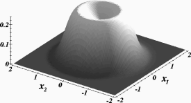
Figure 10: Probability distribution $P_{0}(\rho)$ for a radially symmetric potential in the coordinate space $\{x_{1},x_{2}\}$. The parameters $\alpha,r_{0},v_{0},D$ are set equal to 1.

This distribution is (in the present approximation) universal and valid for any radially symmetric potential of the type specified above. We see that the probability crater is determined by the two deterministic limit cycles (see Fig. 10). The velocity distribution given by Eq. (28) remains to be exact for all radially symmetric potentials. The full stationary probability in the four-dimensional space has the form of two hula hoop distributions Schimansky-Geier et al. (2005); Deng and Zhu (2004). The projections of the distribution onto the $\{x_{1},x_{2}\}$-plane and to the $\{v_{1},v_{2}\}$-plane are two-dimensional rings (see also Fig. 9(a-b)). As in the deterministic case the hula hoop distribution intersects perpendicularly the $\{x_{1},v_{2}\}$-plane and the $\{x_{2},v_{1}\}$-plane. Again, the projections to these planes are rod-like, and the intersection manifold with these planes consists of two ellipses located in the diagonals of the planes Erdmann et al. (2000); Schimansky-Geier et al. (2005). In the deterministic case one of two the rotational motions within the confining potential is excited, this rotation remains a stable solution of the trajectory of one particle. To this rotation belongs a certain value of the angular momentum. For non-vanishing stochastic perturbations, the particle is able to cross the separatrix between the two rotational modes (limit cycles). Due to this ability of the particles one can observe, sometimes, an inversion of the angular momentum of the particle Erdmann et al. (2002). Note that one initial condition will be sufficient to rotate either clockwise or counterclockwise (see Fig. 9(b)).

VII Conclusions

We study here two-dimensional oscillations with nonlinear Rayleigh-type active friction, extending earlier work to

1. oscillations with frequency mismatch

2. oscillations with radially symmetric nonlinear attractive forces.

We investigate several right/left symmetric pairs of limit cycles corresponding to 1:1, 2:1 and 3:1 resonances and their location in the stability regions (Arnold tongues). We show that in the presence of noise the limit cycles are converted into hoops in the four-dimensional space and give analytical estimates for the probability distributions of the coordinates and velocities. Thinking of applications especially for coherent behavior in animal motion on could think of looking for interacting particles where the interaction could be approximated (in mean field approximation) as a deviated parabolic potential. In extention to (Erdmann et al., 2002) on should investigate more the question if there would be any coherent motion which could be located within the higher Arnold tongues. How would the motion of a swarm of particles look than?