Thin front propagation in random shear flows

Abstract

Front propagation in time dependent laminar flows is investigated in the limit of very fast reaction and very thin fronts, i.e. the so-called geometrical optics limit. In particular, we consider fronts evolving in time correlated random shear flows, modeled in terms of Ornstein-Uhlembeck processes. We show that the ratio between the time correlation of the flow and an intrinsic time scale of the reaction dynamics (the wrinkling time $t_{w}$) is crucial in determining both the front propagation speed and the front spatial patterns. The relevance of time correlation in realistic flows is briefly discussed in the light of the bending phenomenon, i.e. the decrease of propagation speed observed at high flow intensities.

Front propagation in fluid flows is a problem relevant to many areas of science and technology ranging from combustion technology W85 to chemistry chem and marine ecology bio . In the last years several theoretical ABP00 ; Const ; KBM01 ; ACVV01 ; ACVV02 ; NX03 ; CTVV03 and experimental LMRS03 ; PH04 ; SS05 ; LMRS05 works studied chemically reactive substances stirred by laminar flows. This problem, though considerably simpler than the case of turbulent flows W85 , is non trivial and displays a very rich and interesting phenomenology. We mention here the front speed locking phenomenon in time dependent cellular flows, which was numerically and theoretically found in Ref. CTVV03 and then experimentally observed in Ref. SS05 . Another interesting example is represented by the theoretical studies on time periodic shear flows KBM01 ; NX03 and the recent experimental work LMRS05 which study aqueous reactions in periodically modulated Hele-Shaw flows.
Laminar flows are interesting also because they constitute a theoretical laboratory to study some problems which can be encountered in more complex (turbulent) flows. For instance, this is the case of time correlations D99 ; A00 that are believed to be very important in determining the bending of turbulent premixed flame velocity when the intensity of turbulence is increased (see Ronney for a discussion about this problem). Actually for bending several mechanisms have been proposed like reaction quenching quench , dynamics of pockets of material which did not react left behind pockets and finally time correlations D99 ; A00 .
The aim of this paper is to investigate the role of time correlations in the propagation of reactions in random shear flows. In particular, we shall consider the problem in the so-called geometrical optics, or Huygens regime Peter that is realized in the case of very fast reactions, taking place in very thin regions. As in Refs.D99 ; A00 , we neglect possible back-effects of the transported reacting scalar on the velocity field, i.e. we treat the problem in the context of passive reactive transport. The latter assumption is justified for dilute aqueous auto-catalytic reactions and more in general for chemical reaction with low heat release. It should be also remarked that in the chosen framework pockets cannot be generated due to shear geometry and quenching of reaction cannot happen due to the choice of working in the geometrical optics limit. Therefore, the case under consideration allows us to focus on the effects due to time correlations solely.
Let us start to introduce our problem by shortly recalling the main equations. Since we consider premixed reactive species, the simplest model consists in studying the dynamics of a scalar field $\theta(\bm{x},t)$ representing the fractional concentration of the reaction’s products ($\theta=1$ inert material, $\theta=0$ fresh one and $0<\theta<1$ coexistence of fresh material and products). The evolution of $\theta$ is ruled by the advection-reaction-diffusion equation:

$$\partial_{t}\bm{u}+\bm{u}\cdot\bm{\nabla}\theta=D\Delta\theta+\frac{f(\theta)}{\tau_{r}}\,,$$ (1)

where $\bm{u}$ is a given velocity field (incompressible $\bm{\nabla}\cdot\bm{u}=0$ through this paper). The $f(\theta)$ (that is typically a nonlinear function with one unstable $\theta=0$ and one stable $\theta=1$ state) models the production process occurring on a time-scale $\tau_{r}$.
Eq. (1) may be studied for different geometries and boundary conditions. In this work we consider an infinite two-dimensional stripe along the x-direction with a reservoir of fresh material on the right, inert products on the left and periodic boundary conditions in the transverse direction (which has size $L$). In particular, we shall be concerned with the concentration initialized as a step, i.e. $\theta(x,y,0)=1$ for $x\leq 0$, and zero otherwise. With this geometry a front of inert material (stable phase) propagates from left to right with an instantaneous velocity which can be defined as:

$$v_{f}(t)=\frac{1}{L}\int_{\mathcal{D}}d\bm{x}\;\partial_{t}\theta(\bm{x},t)\,,$$ (2)

more precisely this is the bulk burning rate Const (integration is over the entire domain $\mathcal{D}$). Most of the theoretical studies aim to predict the dependence of the average front speed $V_{f}=\langle v_{f}\rangle$ on the details of the velocity field. Very important are of course also the propagation speed fluctuations; one would like to predict how these are related to the fluid velocity fluctuations. These are in general very difficult issues, but very important in technological applications, where one has to project the reactor geometry and flow characteristics. Definite answers about the reaction propagation exists only in particular conditions, e.g. when the flow is motionless ($\bm{u}=0$) and under rather general hypothesis on the production function $f(\theta)$ it is possible to show that the reaction asymptotically propagates with a velocity $v_{0}$ within the bounds (see Ref. saarloos for an exhaustive review):

$$2\sqrt{\frac{Df^{\prime}(0)}{\tau_{r}}}\leq v_{0}\leq 2\sqrt{\frac{D}{\tau_{r}}\sup_{\theta}\left\{\frac{f(\theta)}{\theta}\right\}}\,,$$ (3)

where $f^{\prime}$ indicates the derivative, and the thickness of the reaction zone varies as $\xi\propto\sqrt{D\tau_{r}}$. For a wide class of reaction terms $f$, such as the autocatalytic reaction dynamics, $f(\theta)=\theta(1-\theta)$, and more in general for convex functions ($f^{{}^{\prime\prime}}(\theta)<0$) one can prove that $v_{0}=2\sqrt{Df^{\prime}(0)/\tau_{r}}$ exactly. In the presence of a velocity field $\bm{u}$, generally one has that the speed $V_{f}$ is larger than the bare velocity $v_{0}$. Specifically here we consider the limit in which the reaction is much faster than the other time-scales of the problem, formally this regime is reached when $\tau_{r}\to 0$ and $D\to 0$ but with $D/\tau_{r}=const$ such that the bare propagation velocity $v_{0}=2\sqrt{D/\tau_{r}}$ is finite and well defined, while the reaction zone thickness shrinks to zero ($\xi\to 0$) Peter , where for the sake of notation simplicity we posed $f^{\prime}(0)=1$.. It should be noted that this regime, also called geometrical optics limit is commonly encountered in many applications Peter . In this limit, being sharp ($\xi\to 0$), the front dynamics can be described in terms of the evolution of the surface (line in $2d$) which divides inert ($\theta=1$) and fresh ($\theta=0$) material. The effect of the flow is thus to wrinkle the front increasing (in two dimensions) its length $\mathcal{L}_{f}$ and, as a consequence of the relation W85 ; Peter

$$v_{f}=\frac{v_{0}\mathcal{L}_{f}}{L}\,,$$ (4)

(where $L$ is the length of a flat front in the absence of fluid motion) its propagation velocity, i.e. $v_{f}>v_{0}$. Quantifying such an enhancement is one of the main goals of, e.g., the community interested in combustion propagation W85 . It should be also remarked that the presence of complicated flow has also an important role in the generation of patterns, i.e., front spatial structures.
From a formal point of view the evolution of $\theta$ can be recast in terms of the evolution of a scalar field $G({\bf r},t)$, where the iso-line (in 2d) $G({\bf r},t)=0$ represents the front, i.e. the boundary between inert ($G>0$) and fresh ($G<0$) material. $G$ evolves according to the so-called $G$-equation Peter ; EMS95

$$\partial_{t}G+\bm{u}\cdot\bm{\nabla}G=v_{0}|\bm{\nabla}G|\,.$$ (5)

The analytical treatment of this equation is not trivial, and even in relatively simple cases (e.g., shear flows) numerical analysis is needed. Also on the numerical side solving (5) is a non trivial issue, indeed the presence of strong gradients usually requires the regularization of (5) through the introduction of a diffusive term (see e.g. Ald ). Here, following Ref. CTVV03 , we adopt a Lagrangian integration scheme the basic idea of which is now briefly sketched.

Figure 1: Typical front patterns for a stationary shear flow (a), time correlated shear flow with $\tau_{f}=200$ (b) and with $\tau_{f}=2$ (c). In the stationary case $U=1/\sqrt{2}$, while in the time correlated case we set $U_{rms}=\sqrt{2}$. In all cases the bare velocity is $v_{0}=0.2$. For (a) and (b) we used $N_{y}=800$ grid points and $N_{y}=3000$ for (c). Here and in the following figures $L=2\pi$.

First of all let us introduce the type of flow we are interested in, we consider shear flows that can be written as

$$\bm{u}=(U(t)g(y),0)\,,$$ (6)

being $g(y)$ the functional shape of the flow (here $g(y)=\sin(2\pi y/L)$) and $U(t)$ its intensity. The domain of integration is chosen as a stripe $[0:N\,L]\times[0:L]$, where $N$ (typically in the range $5-20$) is the maximum number of cells of size $L$ in the $x$-direction that are used in the integration (the number should be fixed according to the front width). The number of cells $N$ is dynamically adjusted. In particular, after the propagation sets in a statistically stationary regime, while the front propagates the cells on the left that are completely inert with $\theta=1$ are eliminated by the integration domain. On the right side we retain only a finite number (which depends on the maximum allowed speed) of cells with fresh material $\theta=0$. The domain is discretized and the value of $\theta$ in each point of the lattice is updated with the following rule. At each time step, each grid point $\bm{r}_{n,m}=(x_{n},y_{m})$ is backward integrated in time according to the advection by the flow $d\bm{r}/dt=-\bm{u}$. Once the point $\bm{r}^{\prime}$ that will arrive in $\bm{r}_{n,m}$ at time $t$ is known, $\theta(\bm{r}_{n,m},t)$ is set to $1$ if in a circle centered in $\bm{r}^{\prime}$ and having radius $v_{0}dt$ there is at least one grid point with $\theta=1$. This is a straightforward way to implement the Huygens dynamics. The algorithm works as soon as $v_{0}dt$ is sufficiently larger than the spatial discretization $dx=dy=L/N_{y}$ (where $N_{y}$ is the number of grid points in the $y$-direction, and $N_{x}=N\,N_{y}$). For a detailed description of the algorithm see the Appendix in Ref. CTVV03 .

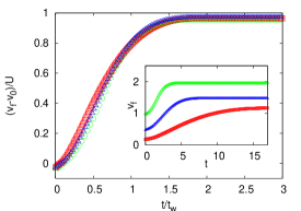
Figure 2: Normalized velocity $V_{n}=(v_{f}(t)-v_{0})/U$ vs $t/t_{w}$ for: $v_{0}=1$, $U=1$ (circles, green online), $v_{0}=0.2$, $U=1$ (squares, red online) and $v_{0}=0.5$, $U=1$ (triangles, blue online). The corresponding $t_{w}$’s were numerically computed as $W_{f}^{\ast}/2U$ obtaining $2.6$, $9.48$ and $18.96$, respectively ($W_{f}^{\ast}$ is estimated by counting the number of pixel in the border between inert and fresh material). The inset shows the unscaled results. The resolution used is $N_{y}=800$.

For a stationary shear flow, i.e. $U(t)=U$, by means of simple geometrical reasonings one can show that at long times the front evolves with velocity ABP00 :

$$V_{f}=v_{0}+U\sup_{y}\{g(y)\}\,,$$ (7)

which, with the choice of the sin flow, means $V_{f}=v_{0}+U$. Similarly one can predict the asymptotic shape of the front, which is shown in Fig. 1a. The important features are the presence of a stationary (maximum) point in correspondence of the point where $g(y)$ has its maximum, and a cusp in its minimum. The asymptotic speed (7) is reached only after the transient time $t_{w}$ necessary to the front shape to reach its maximum length (corrugation). Following KBM01 we call $t_{w}$ as the wrinkling time, that can be defined as the time the front width $\mathcal{W}_{f}$ (i.e. the distance between the leftmost point in which $\theta=0$ and the rightmost in which $\theta=1$) employs to pass from the initial zero-value (indeed at the beginning the front is flat) to the asymptotic one $\mathcal{W}_{f}^{\ast}$. For $U\gg v_{0}$ this time can be estimated as

$$t_{w}\propto L/v_{0}\,.$$ (8)

This comes from the fact that starting from the flat profile the front width $\mathcal{W}_{f}(t)$ grows in time as $2Ut$ up to the moment in which the cusp (see Fig. 1a) is formed (see also KBM01 ). Then the growth slows down up to the stationary value $\mathcal{W}_{f}^{\ast}$. Assuming the linear growth up to the end one may estimate $t_{w}=\mathcal{W}_{f}^{\ast}/(2U)$. Further, since in the shear flow case (where the formation of pockets of inert material is not possible), for $U\gg v_{0}$, the width $\mathcal{W}_{f}^{\ast}$ is proportional to the stationary front length $\mathcal{L}_{f}$, which is linked to the asymptotic velocity by Eq. (4). Finally since the latter given by (7) one ends up with $t_{w}=(L/U)(1+U/v_{0})$ which reduces to (8) for $U\gg v_{0}$. In Fig. 2 we show $v_{f}(t)$ as a function of $t/t_{w}$, as one can see with this rescaling the asymptotic speed is reached at the same instant for systems which have different $U$ and $v_{0}$, as the nice collapse of the different curves indicates (compare with the inset). We noticed that as soon as $U/v_{0}\geq 4$ $t_{w}\propto L/v_{0}$ as predicted by Eq. (8).
The wrinkling time is an inner time scale of the reaction dynamics, which is very important when considering time-dependent flows. In particular, here we study the example of random shear flows (6) with $g(y)=\sin(2\pi y/L)$ (as in the stationary case) and random amplitudes $U(t)$ which are chosen according to an Ornstein-Uhlembeck process. Therefore, $U$ evolves according to the Langevin dynamics

$$\frac{dU}{dt}=-\frac{U}{\tau_{f}}+\sqrt{\frac{2U_{rms}^{2}}{\tau_{f}}}\>\eta$$ (9)

where $\eta$ is a zero-mean Gaussian white noise and $\tau_{f}$ defines the flow correlation time so that $\langle U(t)U(t^{\prime})\rangle=U^{2}_{rms}\exp(-|t-t^{\prime}|/\tau_{f})$. Clearly one has to distinguish two limiting cases: i) when the flow fluctuations are slower than the wrinkling time: $\tau_{f}\gg t_{w}$; ii) when they are much faster: $\tau_{f}\ll t_{w}$.

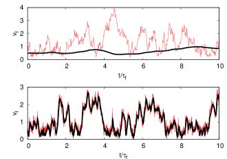
Figure 3: Measured front velocity $v_{f}(t)$ (thick black line) and the adiabatic prediction $v_{0}+|U(t)|$ (solid line, red online) versus $t/\tau_{f}$ for a correlated flow with $U_{rms}=1$, $v_{0}=0.2$ and: (top) $\tau_{f}=200(\gg t_{w}=31.4$), (bottom) $\tau_{f}(2\ll t_{w}=31.4)$. The resolution used was $N_{y}=800$ in the first case and $N_{y}=3000$ in the second one.

$i)$ In this condition the front has enough time for adiabatically adjust itself on the instantaneous flow velocity. Thus by generalizing (7) it is natural to expect that $v_{f}(t)=v_{0}+|U(t)|$ (as confirmed in Fig. 3a) so that $V_{f}=v_{0}+\langle|U(t)|\rangle$. In other words if the velocity fluctuations are slower than the wrinkling time the front can be efficiently corrugated close to the maximal wrinkled shape allowed by the flow and so by (4) can reach maximal speed.
$ii)$ On the other hand in opposite limit $\tau_{f}\ll t_{w}$ the front has not time to be maximally corrugated by the flow, and so its speed cannot reach the maximal amplification allowed by the fluid. In this case it is not anymore true that $v_{f}(t)=v_{0}+|U(t)|$ (see Fig. 3b).
These effects on the propagation speed have a counterpart in the patterns of the front. This is evident by looking at the front shape (compare Fig. 1b and c with a). Indeed while in the case $\tau_{f}\gg t_{w}$ at any instant the shape of front closely resembles that obtained in the stationary case, when $\tau_{f}\ll t_{w}$ one notices that the front length is strongly reduced and the spatial structure complicated by the presence of more than one cuspid.
Looking at Fig. 3b it is clear that the reactive dynamics acts as a sort of filtering of the fluid velocity so that not only the front speed is not enhanced at the maximal allowed value but also its fluctuations are much decreased. In Fig. 4 we show the normalized front speed $V_{n}=(V_{f}-v_{0})/\langle|U(t)|\rangle$ and the normalized variance $\sigma_{n}=\sigma_{f}\/(\sqrt{\langle|U(t)|^{2}\rangle-\langle|U(t)|\rangle^{2}}$ (i.e. the standard deviation of the $v_{f}(t)$ normalized by that expected on the basis of the adiabatic process $|U(t)|$), by fixing the flow intensity $U_{rms}$ and varying the correlation time. Note that in the limit of very long correlation times $V_{n}\approx 1$ and $\sigma_{n}\approx 1$. As one can see a fast drop of the front speed and average fluctuations with respect to its maximum value is observed when $\tau_{f}/t_{w}<1$, confirming the above picture.

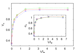
Figure 4: Normalized velocity $V_{n}=(V_{f}-v_{0})/\langle|U|\rangle$ as a function of $\tau_{f}/t_{w}$ for $v_{0}=0.2$ and $U_{rms}=2\sqrt{2}$ (circles, green online), $U_{rms}=\sqrt{2}$ (squares, red online) and $U_{rms}=1/\sqrt{2}$ (triangles, blue online). The inset displays the normalized variance $\sigma_{n}$ in the same cases. The resolution used goes from $N_{y}=3000$ (for the lowest value of $\tau_{f}$) up to 800 (for the highest one).

These results along with those of Refs. D99 ; A00 ; KBM01 confirm the importance of time correlations in the flow in determining the front speed. This may be relevant to more realistic flows in the light of the above cited bending phenomenon. Indeed in turbulent flows one has that at increasing the turbulence intensity fluctuations on smaller and smaller scales appear. These are characterized by faster and faster characteristic time scales. In this respect, as suggested in by the results of this work, one may expect that in the corrugation by these scales become less and less important, so that the average front speed may increase less than expected.
We conclude by noticing that it would be very interesting to test the effects of time-correlations on the front propagation also in other kind of laminar flows. In particular this could be performed in experimental studies in settings similar to those of Refs. LMRS05 where flows of the form $\bm{u}(\bm{r},t)=U(t)\bm{v}(\bm{r})$ can be easily generated with a good control of the time dependence of the amplitude.
We are grateful to C. Casciola for useful discussions. MC and AV acknowledge partial support by MIUR Cofin2003 “Sistemi Complessi e Sistemi a Molti Corpi”, and EU under the contract HPRN-CT-2002-00300.

References

- (1) F. A. Williams, Combustion Theory (Benjamin-Cummings, Menlo Park 1985).
- (2) J. Ross, S. C. Müller, and C. Vidal, Science 240, 460 (1988); I. R. Epstein, Nature 374, 231 (1995).
- (3) E. R. Abraham, Nature 391, 577 (1998); E. R. Abraham et al., Nature 407, 727 (2000).
- (4) B. Audoly, H. Beresytcki and Y. Pomeau, C. R. Acad. Sci. 328, Série II b, 255 (2000).
- (5) P. Constantin, A. Kiselev, A. Oberman and L. Ryzhik, Arch. Rational Mechanics 154, 53 (2000).
- (6) B. Khouider, A. Bourlioux and A.J. Majda, Comb. Th. Model. 5 295 (2001).
- (7) M. Abel, A. Celani, D. Vergni and A. Vulpiani, Phys. Rev. E 64, 046307 (2001).
- (8) M. Abel, M. Cencini, D. Vergni and A. Vulpiani Chaos 12, 481 (2002).
- (9) M. Cencini, A. Torcini, D. Vergni and A. Vulpiani Phys. Fluids 15, 679 (2003).
- (10) J. Nolen and J. Xin, SIAM J. Multiscale Modeling and Simulations 1, 554 (2003).
- (11) M. Leconte, J. Martin, N. Rakotomalala, and D. Salin, Phys. Rev. Lett., 90 128302 (2003).
- (12) M. Leconte, J. Martin, N. Rakotomalala and D. Salin, “Autocatalitic reaction front in a pulsating periodic flow”, preprint arXiv:physics/0504012.
- (13) M. S. Paoletti and T. H. Solomon, Europhys. Lett., 69, 819 (2005).
- (14) A. Pocheau and F. Harambat, in proceedings of the 21th international congress of theoretical an applied mechanics, ICTAM 2004.
- (15) B. Denet, Comb. Th. Model. 3, 585 (1999).
- (16) W.T. Ashurst, Comb. Th. Model 4, 99 (2000).
- (17) P. D. Ronney, in Modeling in Combustion Science, pp. 3-22, Eds. J. Buckmaster and T. Takeno (Springer-Verlag Lecture Notes in Physics, 1994).
- (18) L. Kagan and G. Sivashinshy, Combust, Flame 120, 222 (2000).
- (19) J. Zhu and P.D.Ronney, Combus. Sci. Technol. 100, 183 (1994).
- (20) W. van Saarloos, Phys. Rep., 386, 29 (2003).
- (21) N. Peters, Turbulent combustion (Cambridge University Press, 2000).
- (22) P. F. Embid, A. J. Majda and P. E. Souganidis, Phys. Fluids 7 (8), 2052 (1995).
- (23) R. C. Aldredge, Comb. and Flame 106, 29 (1996).