Wave turbulence and vortices in Bose-Einstein condensation

Abstract

We report a numerical study of turbulence and Bose-Einstein condensation within the two-dimmensional Gross-Pitaevski model with repulsive interaction. In presence of weak forcing localized around some wave number in the Fourier space, we observe three qualitatively different evolution stages. At the initial stage a thermodynamic energy equipartition spectrum forms at both smaller and larger scales with respect to the forcing scale. This agrees with predictions of the the four-wave kinetic equation of the Wave Turbulence (WT) theory. At the second stage, WT breaks down at large scales and the interactions become strongly nonlinear. Here, we observe formation of a gas of quantum vortices whose number decreases due to an annihilation process helped by the acoustic component. This process leads to formation of a coherent-phase Bose-Einstein condensate. After such a coherent-phase condensate forms, evolution enters a third stage characterised by three-wave interactions of acoustic waves that can be described again using the WT theory.

1 Background and motivation

For dilute gases with large energy occupation numbers the Bose-Einstein condensation (BEC) can be described by the Gross-Pitaevsky (GP) equation [1, 2]:

$$i\Psi_{t}+\Delta\Psi-|\Psi|^{2}\Psi=\gamma,$$ (1)

where $\Psi$ is the condensate “wave function” (i.e. the c-number part of the boson annihilation field) and $\gamma$ is an operator which models possible forcing and dissipation mechanisms which will be discussed later. Renewed interest to the nonlinear dynamics described by GP equation is related to relatively recent experimental discoveries of BEC [3, 4, 5]. GP equation also describes light behaviour in media with Kerr nonlinearities. In the nonlinear optics context it is usually called the Nonlinear Schoedinger (NLS) equation.

It is presently understood, in both the nonlinear optics and BEC contexts, that the nonlinear dynamics described by GP equation is typically chaotic and often non-equilibrium [6, 7, 8, 9]. Thus, it is best characterised as “turbulence” emphasizing its resemblance to the classical Navier-Stokes (NS) turbulence. On the other hand, the GP model has an advantage over NS because it has a weakly nonlinear limit in which the stochastic field evolution can be represented as a large set of weakly interactive dispersive waves. A systematic statistical closure is possible for such systems and the corresponding theory is called Wave Turbulence (WT) [10]. For small perturbations about the zero state in the GP model, WT closure predicts that the main nonlinear process will be four-wave resonant interaction. This closure was used in [6, 8, 9] to describe the initial stage of BEC. In the present paper we will examine this description numerically. We report that our numerics agree with the predicted by WT spectra at the initial evolution stage.

It was also theoretically predicted that the four-wave WT closure will eventually fail due to emergence of a coherent condensate state which is uniform in space [9]. At a later stage the condensate is so strong that the nonlinear dynamics can be represented as interactions of small perturbations about the condensate state. Once again, one can use WT to describe such a system, but now the leading process will be a three-wave interaction of acoustic-like waves on the condensate background [9]. Coupling of such acoustic turbulence to the condensate was considered in [11] which allowed to derived the asymptotic law of the condensate growth. However, this picture relies on assumptions that the system will consist of a uniform condensate and small perturbations. Neither the condensate uniformity nor the smallness of perturbations have ever been validated before. In the present paper we will examine whether it is true that the late stage of GP evolution can be represented as a system of weakly nonlinear acoustic waves about strong quasi-uniform condensate. By examining the frequency-wave number Fourier transforms, we do observe waves with frequency in agreement with the Bogoliubov dispersion relation. The width of the frequency spectrum is narrow enough for these waves to be called weakly nonlinear.

A big unresolved question in the theory of GP turbulence has remained about the stage of transition from the four-wave to the tree-wave regimes. This stage is strongly nonlinear and, therefore, cannot be described by WT. However, using direct numerical simulations of equation (1), we show that the transitional state involves a gas of annihilating vortices. When the number of vortices reduces so that the mean distance between the vortices becomes greater than the vortex core radius (healing length) the dynamics becomes strongly nonlinear. This corresponds to entering the Thomas-Fermi regime when the mean nonlinearity is greater than the dispersive term in the GP equation. The mean inter-vortex distance is a measure of the correlation length of the phase of $\Psi$ and, therefore, the vortex annihilation corresponds to creation of a coherent-phase condensate. At this point, excitations with wavelengths in between of the vortex-core radius and the inter-vortex distance behave as sound. In this paper, we draw attention to the similarity of this transition process to the Kibble-Zurek mechanism of the second-order phase transition in cosmology [12, 13].

2 WT closure and predictions

The WT closure is based on the assumptions of small nonlinearity and of random phase and amplitude variables. To show how these assumptions come about we reproduce several essential steps of the kinetic equation derivation. Let us consider GP equation (1) in a periodic box and write it in the Fourier space:

$$i\partial_{t}\hat{\Psi}_{k}-k^{2}\hat{\Psi}_{k}=\sum_{\alpha,\mu,\nu}\bar{\hat{\Psi}}_{\alpha}\hat{\Psi}_{\mu}\hat{\Psi}_{\nu}\delta^{k\alpha}_{\mu\nu}+\hat{\gamma}_{k},$$ (2)

where $\hat{\Psi}_{j}=\hat{\Psi}({\bf k}_{j})$, overbar means complex conjugation, wave vectors ${\bf k}_{j}\;(j=1,2,3)$ are on a 2D grid (due to periodicity) and symbol $\delta^{k\alpha}_{\mu\nu}=1$ for ${\bf k}+{\bf k}_{\alpha}={\bf k}_{\mu}+{\bf k}_{\nu}$ and equal to 0 otherwise.

2.1 Four-wave interaction regime

In order to describe the WT theory for equation (2) we will neglect the forcing/dissipation term $\hat{\gamma}_{k}$ assuming that those are localized at high or low wave numbers and we are mainly interested in an inertial range of ${\bf k}$. Let us make a transformation to the interaction representation variables $a_{k}$ which absorb the linear dynamics and oscillations due to the diagonal terms ${\bf k}={\bf k}_{2}$ and ${\bf k}_{1}={\bf k}_{3}$,

$$a_{k}=e^{i\omega_{k}t+i\int\omega_{nl}\,dt}\Psi_{k},$$ (3)

where $\omega_{k}=k^{2}$ is the linear frequency and

$$\omega_{nl}=\sum_{\bf k}|\hat{\Psi}_{k}|^{2}$$ (4)

is the nonlinear frequency shift. In terms of $a_{k}$ we have

$$i\partial_{t}a_{k}=\sum_{\alpha\neq\mu,\nu}\bar{a}_{\alpha}a_{\mu}a_{\nu}\,\delta^{k\alpha}_{\mu\nu}\,e^{i\omega^{k\alpha}_{\mu\nu}\,t},$$ (5)

where $\omega^{k\alpha}_{\mu\nu}=\omega_{k}+\omega_{\alpha}-\omega_{\mu}-\omega_{\nu}$. The nonlinear frequency drops out from this expression because it is $k$-independent. Small nonlinearity allows to separate the linear and nonlinear timescales. Let us consider solution $a_{k}(T)$ at an intermediate (between linear and nonlinear) time $T\gg 2\pi/\omega_{k}$ but such that changes in $a_{k}$ are still small. We seek this solution as a series

$$a_{k}=a_{k}^{(0)}+a_{k}^{(1)}+a_{k}^{(2)}+...$$ (6)

which is obtained by recursive substitution into (5). For example, $a_{k}^{(0)}=a_{k}|_{T=0}$ and

$$a_{k}^{(1)}(T)=-i\sum_{\alpha\mu\nu}\bar{a}_{\alpha}^{(0)}a_{\mu}^{(0)}a_{\nu}^{(0)}\delta^{k\alpha}_{\mu\nu}\Delta^{k\alpha}_{\mu\nu}.$$ (7)

where $\Delta^{l\alpha}_{\mu\nu}=({e^{i\omega^{l\alpha}_{\mu\nu}T}-1})/{i\omega^{l\alpha}_{\mu\nu}}.$ For the second iteration we get

$$a_{k}^{(2)}(T)=\sum_{\alpha\neq\mu,\nu;u\neq v,\beta}\left(\delta^{\mu\nu}_{\alpha u}\delta^{ku}_{v\beta}a_{\alpha}^{(0)}a_{v}^{(0)}a_{\beta}^{(0)}\bar{a}_{\mu}^{(0)}\bar{a}_{\nu}^{(0)}E(\omega^{k\mu\nu}_{\alpha v\beta},\omega^{ku}_{v\beta})-2\delta^{\alpha v}_{\mu\nu}\delta^{ku}_{v\beta}\bar{a}_{\alpha}^{(0)}\bar{a}_{u}^{(0)}a_{\mu}^{(0)}a_{\nu}^{(0)}a_{\beta}^{(0)}E(\omega^{k\alpha u}_{\mu\nu\beta},\omega^{ku}_{v\beta})\right),$$ (8)

where $E(x,y)=\int_{0}^{T}\Delta(x-y)e^{iyt}dt.$ Expressions (7) and (8) are sufficient for writing the leading order (in small nonlinearity) for the evolution of the spectrum, $n_{k}=\langle|a_{k}|^{2}\rangle$:

$$\dot{n}_{k}=(\langle|a_{k}(T)|^{2}\rangle-\langle|a_{k}(0)|^{2}\rangle)/T={1\over T}(\langle a_{k}^{(0)}\bar{a}_{k}^{(1)}\rangle+\langle a_{k}^{(1)}\bar{a}_{k}^{(0)}\rangle+\langle a_{k}^{(0)}\bar{a}_{k}^{(2)}\rangle+\langle a_{k}^{(2)}\bar{a}_{k}^{(0)}\rangle+\langle|a_{k}^{(1)}|^{2}\rangle).$$ (9)

Here, we must substitute expressions (7) and (8) and perform averaging over the ensemble of initial fields $a_{k}^{(0)}$. For this, we will use a generalized RPA (Random Phase and Amplitude) approach introduced in [14] and which is different from the traditional RPA (Random Phase approximation, see e.g. [10]) by emphasizing randomness of the amplitudes and not only the phases. Namely, we represent complex amplitudes as $a_{k}^{(0)}=A_{k}\psi_{k}$ where $A_{k}$ are positive real amplitudes and $\psi_{k}$ are phase factors taking values on the unit circle on the complex plane. Generalized RPA says that the initial wave field is such that all of its amplitudes $A_{k}$ and phase factors $\psi_{k}$ make a set of independent random variables and that $\psi_{k}$’s are uniformly distributed on the unit complex circle (distribution of $A_{k}$’s need not be specified).

RPA allows to close equations for the spectrum (9) by using the Wick-type splitting of the higher Fourier moments in terms of the spectrum. The first two terms in (9) contain three $a^{(0)}$’s each and, therefore, vanish due to the phase randomness. The other three terms, after substitution of (7) and (8), RPA averaging and taking the large-box and large $T$ limits, give (see details e.g. in [14]):

$$\dot{n}_{k}=4\pi\int n_{k}n_{u}n_{\mu}n_{\nu}\left({1\over n_{k}}+{1\over n_{u}}-{1\over n_{\mu}}-{1\over n_{\nu}}\right)\delta(\omega^{ku}_{\mu\nu})\delta^{ku}_{\mu\nu}\,d{\bf k}_{u}d{\bf k}_{\mu}d{\bf k}_{\nu}.$$ (10)

This is the wave-kinetic equation (WKE) which is the most important object in the wave turbulence theory (for the GE equation, it was first derived in [7]). It contains Delta functions for four wave vectors, $\delta^{ku}_{\mu\nu}=\delta({\bf k}+{\bf k}_{u}-{\bf k}_{\mu}-{\bf k}_{\nu})$, and for the four corresponding frequencies, $\delta(\omega^{ku}_{\mu\nu})$, which means that the spectrum evolution in this case is driven by a 4-wave resonance process. Note that WT approach is applicable not only to the spectra but also to the higher moments and even the probability density functions [14, 15]. However, we are not going to reproduce these results because their study is beyond the aims of the present paper.

There are four power-law solutions of the 4-wave kinetic equation in (10) and they are related to the two invariants for such systems, the total energy, $E=\int\omega_{k}n_{k}d{\bf k}$, and the total number of particles, $N=\int n_{k}d{\bf k}$. Two of such power-law solutions correspond to a thermodynamic equipartition of one of these invariants,

$$n_{k}\sim 1/\omega_{k} = k^{-2}\;\;\;\;\;\hbox{(energy equipartition)},$$ (11)

$$n_{k}\;\;\; = \hbox{const}\;\;\;\hbox{(particle equipartition)}.$$ (12)

These two solutions are limiting cases of the general thermodynamic distribution,

$$n_{k}=T/(\omega_{k}+\mu),$$ (13)

where constants $T$ and $\mu$ have meanings of temperature and chemical potential respectively. Due to isotropy, it is convenient to deal with an angle-averaged 1D wave action density in variable $k=|{\bf k}|$, so called 1D wave action spectrum $N_{k}=2\pi kn_{k}$. In terms of $N_{k}$, solutions (11) and (12) have exponents $-1$ and $1$ respectively.

The other two power-law solutions correspond to a Kolmogorov-like constant flux of either energy (down-scale cascade) or the particles (up-scale cascade) [9]. As shown in [9], the formal solution for the inverse cascade has wrong sign of the particle flux and is, therefore, irrelevant. On the other hand, the power exponent of the direct cascade solution formally coincides with the energy equipartition exponent $-2$ and, in fact, it is the same solution. Because of such a coincidence, the energy flux value is equal to zero on such a solution and, therefore, it is more appropriate to associate it with thermodynamic equilibrium rather than a cascade.

2.2 Three-wave interaction regime

If the system is forced at large wave numbers and there is no dissipation at low $k$’s then there will be condensation of particles at large scales. The condensate growth will eventually lead to a breakdown of the weak nonlinearity assumption [9, 17] and the 4-wave WKE (10) will become invalid for describing subsequent evolution. On the other hand, it was argued in [9] that such late evolution one can consider small disturbances of coherent condensate state $\Psi_{0}=$ const, so that a WT approach can be used again (but now on a finite-amplitude background),

$$\Psi({\bf x},t)=\Psi_{0}\,(1+\phi({\bf x},t)),\;\;\;\;\phi\ll\Psi_{0}.$$ (14)

Then, with respect to condensate perturbations $\phi$, the linear dynamics has to be diagonalised via the Bogoljubov transformation, which in our case is [9, 16, 11]

$$\hat{\phi}_{k}={1\over 2\sqrt{\rho_{0}}}\left[\left({k\over\omega_{k}^{1/2}}+{\omega_{k}^{1/2}\over k}\right)a_{k}+\left({k\over\omega_{k}^{1/2}}+{\omega_{k}^{1/2}\over k}\right)\bar{a}_{k}\right],$$ (15)

where $a_{k}$ are new normal amplitudes (see for example [11]). In the linear approximation, amplitudes $a_{k}$ oscillate at frequency

$$\omega_{k}=k\sqrt{k^{2}+2\rho_{0}}$$ (16)

which is called the Bogoljubov dispersion relation. For strong condensate, $\rho_{0}\gg k^{2}$, this dispersion relation corresponds to sound.

Because of the non-zero background, the nonlinearity will be quadratic with respect to the condensate perturbations and, thus, the resulting WT closure now gives rise to a 3-wave WKE. This WKE was first obtained in [9] (see also [11]) and here we reproduce it without derivation,

$$\dot{n}_{k}=\pi\int(R_{k12}-R_{1k2}-R_{2k1})\,d{\bf k}_{1}d{\bf k}_{2}\,,$$ (17)

where

$$R_{k12}=|V_{kk_{1}k_{2}}|^{2}\,\delta({{{\bf k}-\bf{k_{1}}-\bf{k_{2}}}})\,\delta({\omega_{{k}}-\omega_{1}-\omega_{2}})\,(n_{1}n_{2}-n_{k}n_{1}-n_{k}n_{2}).$$

Here, $V_{k,k_{1},k_{2}}$ is the interaction coefficient which has the following form

$$V_{k,k_{1},k_{2}}={\Psi_{0}\sqrt{\omega_{k}\omega_{1}\omega_{2}}\over(2\pi)^{3/2}}\left\{{6\over(\alpha_{k}\alpha_{1}\alpha_{2})^{1/2}}+{1\over 2}\left[{({\bf k}\cdot{\bf k_{1}})\over kk_{1}\alpha_{2}}+{({\bf k}\cdot{\bf k_{2}})\over kk_{2}\alpha_{1}}+{({\bf k_{1}}\cdot{\bf k_{2}})\over k_{1}k_{2}\alpha_{k}}\right]\right\}$$ (18)

where

$$\alpha_{k}={2\rho_{0}+k^{2}}.$$ (19)

At late time the condensate becomes strong, $\rho_{0}\gg k^{2}$, and turbulence becomes of acoustic type. The number of particles is not conserved by the turbulence alone (particles can be transferred to the condensate) and there are only two relevant power-law solutions in this case: thermodynamic equipartition of energy and the energy cascade spectrum. Because of isotropy, one often considers 1D (i.e. angle-integrated) energy density,

$$E(k)=2\pi k\omega_{k}n_{k}.$$ (20)

In terms of this quantity, the thermodynamic spectrum is

$$E(k)\sim k,$$ (21)

and the energy cascade spectrum is

$$E(k)\sim k^{-3/2}.$$ (22)

Note that the energy cascade is direct and the corresponding spectrum can be expected in $k$’s higher than the forcing wave number, whereas the thermodynamic spectrum is expected at the low-$k$ range to the left of the forcing [11].

Note that the described above picture of acoustic WT relies on two major assumptions.

1. Condensate is coherent enough so that its spatial variations are slow and it can be treated as uniform when evolution of the perturbations about the condensate is considered. In the other words, a scale separation between the condensate and the perturbations occurs.

2. Coherent condensate is much stronger than the chaotic acoustic disturbances. This allows to treat nonlinearity of the perturbations around the condensate as small.

Both of these assumptions have not been validated before and their numerical check will be one of our goals. Another major goal will be to study the transition stage that lies in between of the 4-wave and the 3-wave turbulence regimes. This transition is characterised by strong nonlinearity and the role of numerical simulations becomes crucially important in finding its mechanisms.

Once the 3-wave acoustic regime has been reached, the condensate continues to grow due to a continuing influx of particles from the acoustic turbulence to the condensate. This evolution, where an unsteady condensate is coupled with acoustic WT, was described in [11] who predicted that asymptotically the condensate grows as $\rho_{0}\sim t^{2}$ if the forcing is of an instability type $\hat{\gamma}=\nu_{k}n_{k}$. However, in the present paper we work with a different kind of forcing which is most convenient and widely used in numerical simulations: we keep amplitudes in the forcing range fixed (and we chose their phases randomly). Thus, one should not expect observing the $t^{2}$ regime predicted in [11] in our simulations. Note that 2D NLS turbulence was simulated numerically with specific focus on the condensate growth rate in [18]. In our work, we do not aim to study the condensate growth rate because it is strongly dependent on the forcing type which, in our model, is quite different from turbulence sources in laboratory. On the other hand, we believe that the main stages of the condensation, i.e. transition from a 4-wave process, through vortex annihilations, to 3-wave acoustic turbulence, are robust under a wide range of forcing types.

3 Setup for numerical experiments

In this paper we consider a setup corresponding to homogeneous turbulence and, therefore, we ignore finite-size effects due to magnetic trapping in BEC or to the finite beam radii in optical experiments. For numerical simulations, we have used a standard pseudo-spectral method for the 2D equation (1). The number of grid points in physical space was set to $N\times N$ with $N=256$. Resolution in Fourier space was $\Delta k=2\pi/N$. Sink at high wave numbers was provided by adding to the right hand side of equation (1) the hyper-viscosity term $\nu(-\nabla^{2})^{n}\psi$. Values of $\nu$ and $n$ were selected in order to localized as much as possible dissipation to high wave numbers but avoiding at the same time the bottleneck effect. We have found, after a number of trials, that $\nu=2\times 10^{-6}$ and $n=8$ were good choices for our purposes. In some simulations, we have also used a dissipation at low wave numbers of the form of $\nu(-\nabla^{2})^{-n}\psi$ with $\nu=1\times 10^{-18}$ and $n=8$. This was done, e.g., to see what changes if one suppresses the condensate formation. Forcing was localized in Fourier space and was chosen as $f=|f|exp[-i\phi(t)]$ with $|f|$ constant in time and $\phi(t)$ randomly selected between 0 and $2\pi$ each time step. i) To study turbulence in the down-scale inertial range we force the system isotropically at wave numbers $4\Delta k\leq|k|\leq 6\Delta k$. To avoid condensation at large scales we introduce a dissipation at low wave numbers, as was previously explained. ii) To study the condensation we chose forcing at wave numbers $60\Delta k\leq|k|\leq 63\Delta k$ and dissipation at all higher wave numbers. A number of numerical simulations were performed both with and without the dissipation at the low wave numbers. Time step for integration was $t=0.1$ and usually $10^{5}$ time steps have been performed for each simulation. This is usually enough for reaching a steady state when dissipation at both high and low wave numbers was placed.

4 Numerical results

4.1 Turbulence with suppressed condensation

We start with a state without condensate for which WT predicts four-wave interactions. WKE has two conserved quantities in this case, the energy and the particles, and the directions of their transfer in the scale space must be opposite to each other. Indeed, let us assume that energy flows up-scale and that it gets dissipated at a scale much greater than the forcing scale. This would imply dissipating the number of particles which is much greater than what was generated at the source (because of the factor $k^{2}$ difference between the energy and the particle spectral densities). This is impossible in steady state and, therefore, energy has to be dissipated at smaller (than forcing) scales. On the other hand, the particles have to be transferred to larger scales because dissipating them at very small scales would imply dissipating more energy than produced by forcing. This speculation is standard for the systems with two positive quadratic invariants, e.g. 2D Euler turbulence where one invariant, the energy, flows up-scale and another one, the enstrophy, flows down-scale.

Thus, ideally, one would like to place forcing at an intermediate scale and have two inertial ranges, up-scale and down-scale of the source. However, this setup is unrealistic because the presently available computing power would not allow us to achieve simultaneously two inertial ranges wide enough to study scaling exponents. Therefore, we split this problem to two, with forcing at the left and at the right ends of a single inertial range.

4.1.1 Turbulence down-scale of the forcing

Our first numerical experiment is designed to test the WT predictions about the turbulent state corresponding to the down-scale range with respect to the forcing scale. Thus we chose to force turbulence at large scales and to dissipate it at the small scales as described in the previous section. Our results for the one-dimensional wave action spectrum is statistically stationary condition is shown in Figure 1. We see a range with slope $-1$ predicted by both the Kolmogorov-Zakharov (KZ) energy cascade and the thermodynamic energy equipartition solutions of the four-wave WKE. As we mentioned earlier, it would be more appropriate to interpret this spectrum as a quasi-thermodynamic state rather than the KZ cascade because the energy flux expression formally turns into zero at the power spectrum with $-1$ exponent. We emphasise, however, that the state here is quasi-thermodynamic with a small flux component present on thermal background because of the presence of the source and sink. One could compare this state to a lake with two rivers bringing the water in and out of the lake. In comparison, pure KZ cascade would be more similar to a waterfall.

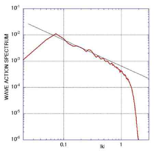
Figure 1: 1D wave action spectrum $N_{k}$ for the down-scale inertial range. A line corresponding to $k^{-1}$, the wave turbulence prediction, is also included.

To check that the waves in our system are indeed weakly nonlinear, we look at the space-time Fourier transform of the wave field. The frequency-wave number plot of this Fourier transform is shown in Figure 2. We see that this Fourier transform is narrowly concentrated near the linear dispersion curve, which confirms that the wave field is weakly nonlinear. We can also see that the spectrum is slightly shifted upwards by a value which agrees with the nonlinear frequency shift found via substitution of the numerically obtained spectrum into (4).

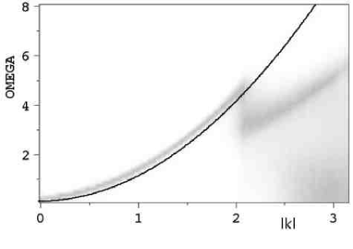
Figure 2: Wave number-frequency distribution of the space-time Fourier transform of $\Psi$ in the down-scale inertial range. Dispersion relation from linear theory is shown in black curve.

4.1.2 Up-scale turbulence

In the up-scale range one could expect that, in analogy with the 2D Navier-Stokes turbulence, there would be an inverse cascade of the number of particles and that the corresponding KZ spectrum would be observed. Nevertheless, it was pointed out in [9] that the analytical KZ spectrum has “wrong” direction of the flux of particles in the 2D GP model and, therefore, cannot form. Our numerics agree with this view. Instead of the KZ, our numerical simulations show that a statistical stationary state with a power law very close to $k^{-1}$ forms, see Figure 3. This solution corresponds to the thermodynamics solution with energy equipartition in the $k$-space.

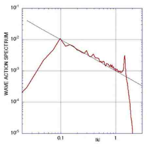
Figure 3: 1D waveaction spectrum $N_{k}$ in the up-scale range. A power law of the form of $k^{-1}$ is also shown.

Note that both theoretical rejection of the particle-cascade spectrum [9] and our numerical study relate to the 2D model and the situation can change in the 3D case. Namely, it is possible that the up-scale dynamics in 3D will be characterised by the particle-flux KZ solution or a more complicated mixed state which involves both cascade and temperature. On the other hand, formation of a pure thermodynamic state in 2D is quite fortunate for the theoretical description because analogies with the theories of phase transition between different types of thermodynamic equilibria become more meaningful.

Here, we also check that the waves in this regime are weakly nonlinear by looking at the space-time Fourier transform. The corresponding frequency-wave number plot is shown in Figure 4. As in the down-scale inertial range, we see that this Fourier transform is narrowly concentrated near the linear dispersion curve, i.e. the wave field is weakly nonlinear in this state.

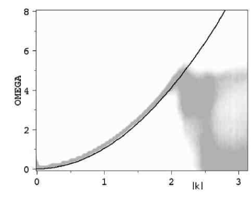
Figure 4: Wave number-frequency distribution of the space-time Fourier transform of $\Psi$ in the up-scale inertial range. Dispersion relation from linear theory is shown in black curve.

4.2 Bose-Einstein condensation

4.2.1 Initial stage: four-wave process

In order to study the stages of the condensation process, the results presented in the following have been obtained with forcing localized at high wave numbers without dissipation at low wave numbers. At the initial stage of the simulation, the nonlinearity remains small compared to the dispersion in the GP equation and the four-wave kinetic equation can be used. In Figure 5, we show the initial (pre-condensate) stages of the spectrum evolution. Similarly to the case where the condensation was suppressed, we observe the formation of a thermodynamic distribution.

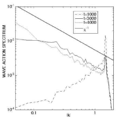
Figure 5: Initial stages of the evolution of the 1D wave action spectrum $N_{k}$. A power law of the form of $k^{-1}$ is also shown.

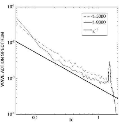
Figure 6: Later stages of the evolution of the 1D wave action spectrum $N_{k}$. A power law of the form of $k^{-1}$ is also shown.

4.2.2 Transition

After the stage where the four-wave interaction dynamics holds, the dynamics is characterised by a transitional stage in which the the low-$k$ front of the evolving spectrum reaches the largest scale (at about $t=5000$), see Figure 6; the spectrum begins to become steeper at low wave numbers and, as expected, the thermodynamics solution does not hold anymore. This behaviour indicates that a change of regime occurs around time $t=5000$. However, the information contained in the spectrum is insufficient to fully characterize this regime change and this brings us to study this phenomenon by measuring several other important quantities.

To get an initial impression of what is happening during the transition stage it is worth to first of all examine the field distributions in the coordinate space. Figure 7 shows a series of frames of the real part of $\Psi$ (imaginary part looks similar). One can see that this field exhibits growth of large-scale structure.

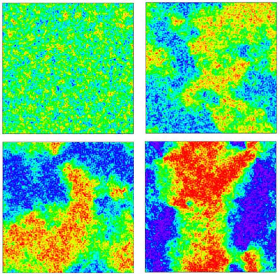
Figure 7: $Re[\psi(x,y)]$ at different times: $t=2500$, $t=5000$, $t=7500$, $t=10000$.

On the other hand, field $|\Psi|$, shown in Figure 8, still remains dominated by small-scale structure. In contrast with $|\Psi|$, field $\Psi$ contains an additional information – the phase.

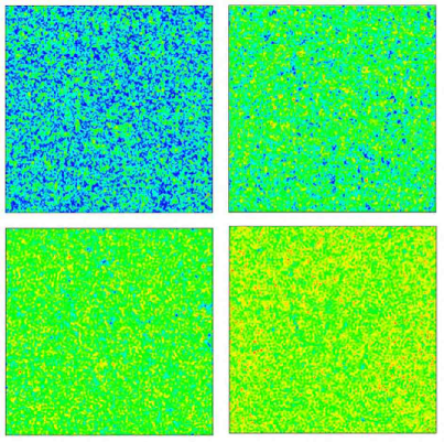
Figure 8: $|\psi(x,y)|$ at different times: $t=2500$, $t=5000$, $t=7500$, $t=10000$.

Thus, separation of the characteristic scales in Figure 7 and 8 can be attributed to the fact that the phase correlation length becomes much longer than the typical wavelength of sound (characterised by fluctuations of $|\Psi|$ as explained above in Section 2.2). This scale separation can also be seen by comparing the spectrum of $|\Psi|$, shown in Figure 9 with the spectrum of $\Psi$ in Figures 5 and 6: one can see that the former is more flat than the later.

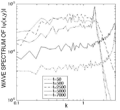
Figure 9: Spectrum for variable $|\psi(x,y)|$ at different times.

Now that we have established that the phase is an important parameter, we can measure its correlation length as the mean distance between the phase defects – vortices. Vortices in the GP model are points in which $\Psi=0$. Some of such points correspond to the $2\pi$ phase increment when one goes once around them, whereas the other points gain $-2\pi$. These vortices can be defined as positive and negative correspondingly. In contrast with the Euler equation of the classical fluid, positive and negative vortices can annihilate in the GP model and they can get created “from nothing”. Figure 10 shows a sequence of plates showing the positive and negative vortex positions at several different moments of time. One can see that initially there were a lot of vortices, which is not surprising because initial field is weak, i.e. close to zero everywhere. However, at later times we see the number of vortices is rapidly dropping, which means that the vortex annihilation process dominates over the vortex-pair creations.

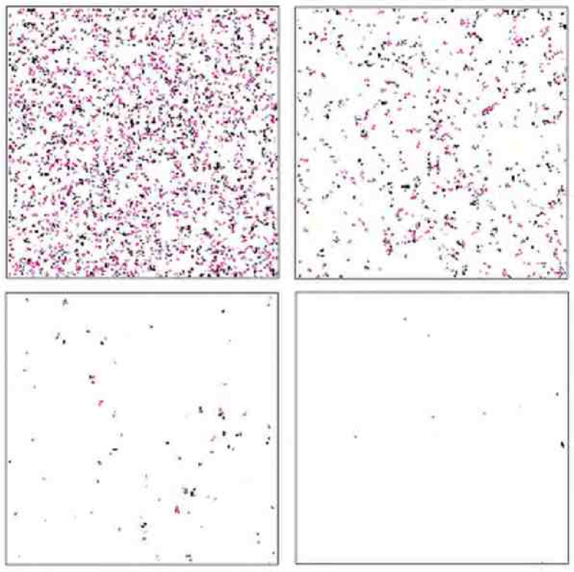
Figure 10: Vortices in the $(x,y)$ plane at different times: $t=2500$, $t=3250$, $t=5000$, $t=7500$.

The total number of vortices (normalised by $N^{2}$) is shown as a function of time in Figure 11, where one can see a fast decay. The law of decay is best seen on the $log-lin$ plot, see Fiigure 12 where one can see a regime

$$N_{vortices}=A-B\log t$$ (23)

with $A=3.36$ and $B=0.9223$ which sets in at $t=800$ to $t=3500$. Thus, the phase correlation distance, being of the order of the mean distance between the vortices, exhibits a fast growth in time.

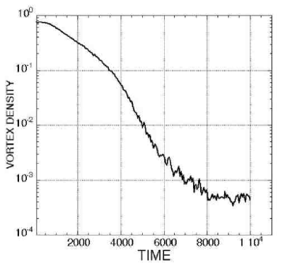
Figure 11: Evolution in time of the density of vortices in a lin-log plot.

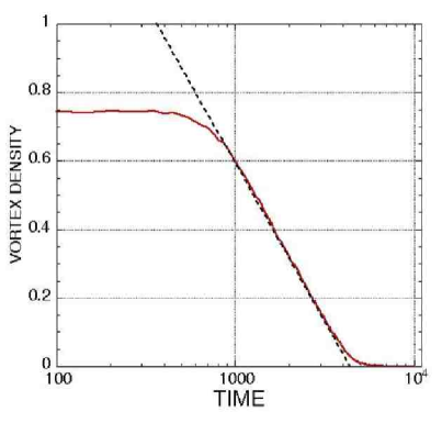
Figure 12: Evolution in time of the density of vortices in a log-lin plot. The dashed line corresponds to the fit $N_{vortices}=3.36-9.223Log(t)$

Let us have a look at a slice of the field $|\Psi|$ through typical vortices at a late time when most of the them have annihilated, see Figure 13. One can see that $|\Psi|$ is close to zero (i.e. both $Re[\psi]$ and $Im[\psi]$ cross zero) at the vortex centres and that it sharply grows to order-one values (“heals”) at small distances from the vortex centres which are much less than the distance between the vortices. This means that these vortices represent fully nonlinear coherent structures each of which can be approximately seen as an isolated Pitaevski vortex solution [2]. In contrast, the initial vortices are too close to each other to be coherent and they correspond to a nearly linear field.

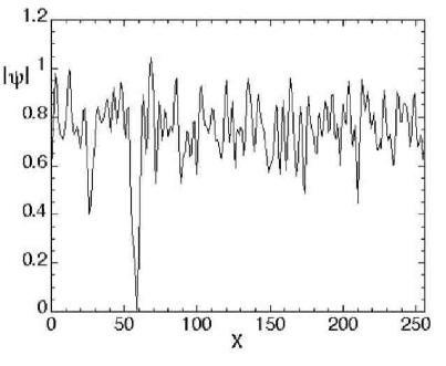
Figure 13: Slice of the field $|\Psi|$ for constant $y$: a single vortex is visible in the plot.

The moment when the mean inter-vortex separation becomes comparable to the healing length can be captured by the intersection point of the graphs for the mean (space averaged) nonlinear and the mean (space averaged) Laplacian terms in the GP equation, see Figure 14.

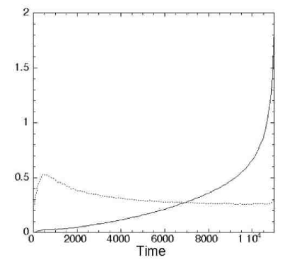
Figure 14: The solid line represents the space-averaged $|\nabla^{2}\psi(x,y)|$; the dotted line is the space-averaged $|\psi(x,y)|^{3}$. See text for comments.

This intersection (at $t=6950$) marks the moment when mean nonlinearity becomes greater than the mean linear dispersion, i.e. the Thomas-Fermi regime sets in. This regime could be thought of as the one of a fully developed condensate when the nonlinearity, when measured with respect to the zero level, is strong and therefore the 4-wave WT description breaks down. However, as we will see in the next section, we now have weakly nonlinear perturbations if they are measured with respect to a non-zero condensate state. Evolution of such perturbations takes form of three-wave acoustic turbulence.

What makes vortices annihilate? A positive-negative vortex pair, when taken in isolation, would propagate with constant speed without changing the distance between the vortices [23]. Thus, there should be an additional entity which could exchange energy and momentum with the vortex pair and to allow them annihilate. We note that the field $|\Psi|$ is very “choppy” in the region between the vortices, see figure (13), and, therefore, it is natural to conjecture that the missing entity is sound. To check this conjecture, we perform the following numerical experiment. At a desired time we filter the field and let it evolve further without sound. The filtering is performed numerically in the following way: we have used a Gaussian filter in physical space and have smoothed the field around vortices. The complex field $\psi$ is therefore convoluted with a normalised Gaussian function with standard deviation much smaller with respect to the mean distance between vortices. The filter is applied only in the region where no vortices are located. The result of the filtering procedure on the evolution of the number of vortices is shown in Figure 15. We see that removing the sound component does indeed reverse the vortex annihilation process and for some time (until new sound gets generated from forcing) we observe that the vortex creation process dominates.

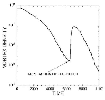
Figure 15: Evolution of the vortex density in time. At time $t=6500$, sound has been filtered according to the methodology described in the text.

We point out that the described above regime change, accompanied by vortex annihilations, is very similar to the Kibble-Zurek mechanism of the second-order phase transition in cosmology [12, 13]. This mechanism suggest that at an early inflation stage, Higgs fields experience a symmetry breaking transition from “false” to “true” vacuum, and this transition is accompanied by a reconnection-annihilation of “cosmic strings” which are 3D analogs of the 2D point vortices considered in this paper. To describe these fields, one normally uses nonlinear equations of so-called Abbelian model [21], but the non-linear Klein-Gordon or even the GP equation are sometimes used as simple models in cosmology which retain similar physics [21, 22].

4.2.3 Late condensation stage: acoustic turbulence

It was predicted in [9] that the turbulent condensation in the GP model will lead to creation of a strong coherent mode with $k=0$ such that the excitations at higher wave numbers would be weak compared to this mode. If this is the case, one can expand the GP equation about the new equilibrium state, uniform condensate, use Bogoljubov transform to find new normal modes and a dispersion relation for them, equation (15), and to obtain a new WKE for this system that would be characterised by by three-wave interactions, (17). However, as we saw in Figure 6 the peak at small $k$ remains quite broad that is the coherent condensate, if present, remains somewhat non-uniform. Despite of this non-uniformity, one can still use the approach of [9] if there is a scale separation between the condensate coherence length (intervortex distance) and the sound wavelength and if the sound amplitude is much smaller than the one of the condensate.

We have already seen tendency to the scale separation in figures 6, 7, 8, 9. On the other hand, smallness of the sound intensity can be seen in figure 16 which compares (space-averaged) $<|\Psi|^{2}>$ and $<|\Psi|>^{2}$. We see that at the late stages these quantities have very close values which means that the deviations of $|\Psi|$ from its mean value (condensate) are weak. Thus, both conditions for the weak acoustic turbulence to exist are satisfied at the late stages.

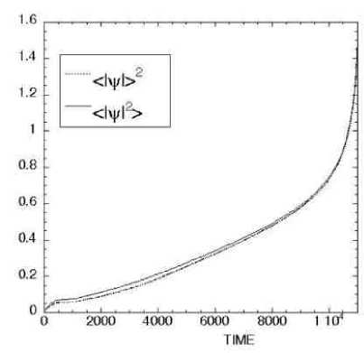
Figure 16: Evolution in time of $<|\Psi|^{2}>$ and $<|\Psi|>^{2}$.

However, the best way to check if the condensate perturbations do behave like weakly nonlinear sound waves obeying the Bogoljubov dispersion relation consists in plotting the square of the absolute value of the space-time Fourier transform of $\Psi$. This result is given in Figure 17 for the latest stage of the simulation (from time $t=10488$ to $t=11000$). Note that for each $k$ the spectrum has been divided by its maximum in order to be able to follow the dispersion relation up to high wave numbers.

The normal variable for the Bogoljubov sound is given in terms of $\psi$ by expressions (14) and (15) , and, therefore, when plotting the Bogoljubov dispersion (16), we should add a constant frequency of the condensate oscillations, $\omega_{0}=\langle|\Psi|^{2}\rangle$.

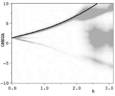
Figure 17: Dispersion relation calculated from numerical simulation compared with the upper branch of the Bogoljubov dispersion relation (solid line)

One can see that the main branch of the spectrum does follow the Bogoljubov law up to the wave numbers which correspond to the dissipation range. Further, the wave distribution is quite narrowly concentrated around the Bogoljubov curve which indicates that these waves are weakly nonlinear. Note that the lower branch in Figure 17 is related to the $\bar{a}_{k}$ contribution to expression (15) which vanishes at larger $k$. Importanlty, we can also see the middle (horizontal) branch with frequency $\omega_{0}$ which quickly fades away at finite $k$’s and which corresponds to the coherent large-scale condensate component.

Now let us consider the energy spectrum. The GP Hamiltonian can be written in terms of both real and Fourier quantities,

$$H=\int(|\nabla\Psi|^{2}+{1\over 2}|\Psi|^{4})\,d{\bf x}=\int(k^{2}|\hat{\Psi}|^{2}+{1\over 2}|\hat{\rho}|^{2})\,d{\bf k},$$ (24)

where $\rho=|\Psi|^{2}.$ Thus, we measure the 1D energy spectrum in this case as $E(k)=E_{1}(k)+E_{2}(k)$ with $E_{1}(k)=k^{3}|\hat{\Psi}|^{2}$ and $E_{2}(k)={k\over 2}|\hat{\rho}|^{2}$

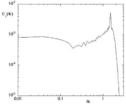
Figure 18: $E_{1}(k)$ at the latest stage of the simulation (see equation (24)).

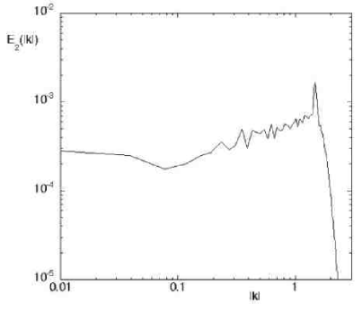
Figure 19: $E_{2}(k)$ at the latest stage of the simulation (see equation (24)).

The contributions to the energy spectrum $E_{1}$ and $E_{2}$ as well as the total spectrum $E(k)$ at a time corresponding to the acoustic regime are shown in figures 18, 19 and 20 respectively.

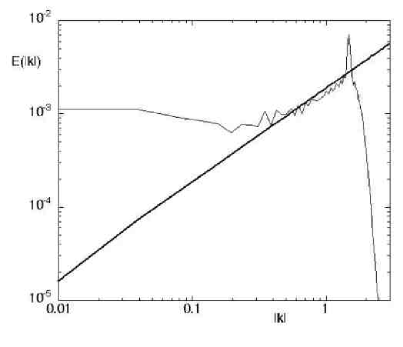
Figure 20: $E(k)=E(k_{1})+E(k_{2})$ at the latest stage of the simulation (see equation (24))

We see that at small scales the total energy spectrum $E(k)$ scales as $1/k$ which is a thermodynamic energy equipartition solution in this case.

5 Conclusions

Firstly, we confirmed WT predictions of the energy spectra in the down-scale and up-scale inertial intervals in the cases when the fluxes are absorbed by dissipation in the end of the inertial interval (so that no condensation or build-up is happening). In both of these cases we observed spectra with an exponent corresponding to the energy equipartition thermodynamic solution $N_{k}\sim 1/k$ (which formally coincides with the exponent for the energy cascade solution). By looking at the shape of the frequency-wave number mode distributions, we verified that the turbulence is weak.

Secondly, we studied a system without dissipation at large scales. We observed a process of Bose-Einstein condensation and formation of a coherent large-scale mode which happens via annihilating vortices. This scenario is similar to the Kibble-Zurek phase transition in cosmology which involves annihilating cosmic strings. We established that the process of the vortex annihilation is due to the presence of sound. The condensate correlation length, which in our case is of the order of the mean inter-vortex distance, turns into infinity in a finite time as $\lambda\sim 1/(\log t^{*}-\log t)^{1/2}$, see equation (23).

We confirmed numerically that in late condensation stages the system can be described as a weakly nonlinear acoustic turbulence on the background of a quasi-uniform coherent condensate. Namely, we confirmed that the wave excitations are narrowly distributed around the Bogoljubov dispersion law, i.e. that the turbulence is (i) acoustic and (ii) weak. We observed a spectrum that corresponds to the energy equipartition solution of the 3-wave kinetic equation for such acoustic turbulence.

An interesting question to be addressed in future is to what extend the findings of this work are relevant to the 3D GP model. We can speculate that the energy spectra may have a different nature in 3D and, in particular, may expect formation of the Kolmogorov-like spectra corresponding to the energy and the particle cascades. On the other hand, it is reasonable to expect that the Kibble-Zurek scenario of condensation will persist in the 3D case, i.e. the correlation length will grow because of the reconnecting and shrinking vortex loops. It is also likely that such vortex loop shrinking will be facilitated by the sound component. Computations of 3D GP equation in a non-turbulent setting were done in [24] where such processes as vortex reconnection and the role of the acoustic component were considered. Turbulent setting will be more taxing on the computing resources due to the great variety of scales involved and, therefore, necessity of high resolution and long computation times.

Acknowledgments
We thank Al Osborne for discussions in the early stages of the work.

References

- [1] E.P. Gross, Structure of a quantized vortex in boson systems, Nuovo Cimento, 20, 454, (1961).
- [2] L.P. Pitaevsky, Vortex lines in an imperfect Bose gas, Sov. Phys. JETP, 13, 451 (1961).
- [3] M. H. Anderson, J.R. Ensher, M.R. Matthews, C.E. Wieman, E.A. Cornell, Observation of Bose-Einstein Condensation in a Dilute Atomic Vapor, Science 269, 198 (1995).
- [4] C. C. Bradley, C. A. Sackett, J. J. Tollett, and R. G. Hulet, Evidence of Bose-Einstein Condensation in an Atomic Gas with Attractive Interactions, Phys. Rev. Lett, 75, 1687-1690 (1995).
- [5] K. B. Davis, M. -O. Mewes, M. R. Andrews, N. J. van Druten, D. S. Durfee, D. M. Kurn, and W. Ketterle, Bose-Einstein Condensation in a Gas of Sodium Atoms, Phys. Rev. Lett, 75 3969, (1995).
- [6] Yu.M. Kagan, B.V. Svistunov and G.P. Shlyapnikov, Kinetics of Bose condensation in an interacting Bose gas, Sov. Phys. JETP, 75, 387, (1992).
- [7] V.E. Zakharov, S.L. Musher, A.M. Rubenchik, Hamiltonian approach to the description of nonlinear plasma phenomena Phys. Rep. 129, 285 (1985).
- [8] D.V. Semikoz and I.I. Tkachev, Kinetics of Bose Condensation, Phys. Rev. Lett. 74, 3093 3097 (1995).
- [9] A. Dyachenko, A.C. Newell, A. Pushkarev, V.E. Zakharov, Optical turbulence: weak turbulence, condensates and collapsing filaments in the nonlinear Schroödinger equation, Physica D 57, 96 (1992).
- [10] V.E. Zakharov, V.S. L’vov and G.Falkovich, Kolmogorov Spectra of Turbulence, Springer-Verlag, 1992.
- [11] V.E.Zakharov and S.V. Nazarenko, Dynamics of the Bose-Einstein condensation, Physica D, 201 203-211 (2005).
- [12] T.W.B. Kibble, Topology of cosmic domains and strings, J. Phys. A: Math. Gen. 9, 1387 (1976).
- [13] W.H. Zurek, Cosmological experiments in superfluid helium?, Nature 317 505 (1985); Acta Physica Polonica B24 1301 (1993).
- [14] Y. Choi, Yu. Lvov, S.V. Nazarenko and B. Pokorni, Anomalous probability of large amplitudes in wave turbulence, Physics Letters A, 339, Issue 3-5, p. 361-369 (arXiv:math-ph/0404022 v1 Apr 2004). Y. Choi, Yu. Lvov and S.V. Nazarenko, Joint statistics of amplitudes and phases in Wave Turbulence, Physica D Vol 201 121-149 (2005).
- [15] Yu. Lvov and Sergey Nazarenko, “Noisy” spectra, long correlations and intermittency in wave turbulence, Phys. Rev. E 69, 066608 (2004) (2004). Also at http://arxiv.org/abs/math-ph/0305028.
- [16] Yuri V.Lvov, Sergey Nazarenko and Robert West, Wave turbulence in Bose-Einstein condensates, Physica D 184 333-351 (2003).
- [17] L. Biven, S.V. Nazarenko and A.C. Newell, Breakdown of wave turbulence and the onset of intermittency, Phys. Lett. A, 280, 28-32, (2001); A.C. Newell, S.V. Nazarenko and L. Biven, Physica D, 152-153, 520-550, (2001).
- [18] A. Dyachenko , G. Falkovich Condensate turbulence in two dimensions, Phys. Rev. E 54, 5095 (1996).
- [19] C. Connaughton, C. Josserand, A. Picozzi, Y. Pomeau, S. Rica,Condensation of classical nonlinear waves, (2005-02-21) oai:arXiv.org:cond-mat/0502499, 2005
- [20] M. Tsubota, K. Kasamatsu, and M. Ueda, Vortex lattice formation in a rotating Bose-Einstein condensate Phys. Rev. A 65, 023603 (2002).
- [21] J.A. Peacock, “Cosmological Physics”, Cambridge University Press (1999).
- [22] W.H. Zurek, Cosmological Experiments in Condensed Matter Systems, Phys. Rept. 276 177-221 (1996).
- [23] C.A. Jones and P.H. Roberts, Motions in a Bose condensate. IV. Axisymmetric solitary waves, J. Phys. A: Math. Gen. 15 2599 (1982).
- [24] N.G. Berloff, Interactions of vortices with rarefaction solitary waves in a condensate and their role in the decay of superfluid turbulence, Phys. Rev A 69 053601 (2004).