Large-scale effects on meso-scale modeling for scalar transport

Abstract

The transport of scalar quantities passively advected by velocity fields with a small-scale component can be modeled at meso-scale level by means of an effective drift and an effective diffusivity, which can be determined by means of multiple-scale techniques. We show that the presence of a weak large-scale flow induces interesting effects on the meso-scale scalar transport. In particular, it gives rise to non-isotropic and non-homogeneous corrections to the meso-scale drift and diffusivity. We discuss an approximation that allows us to retain the second-order effects caused by the large-scale flow. This provides a rather accurate meso-scale modeling for both asymptotic and pre-asymptotic scalar transport properties. Numerical simulations in model flows are used to illustrate the importance of such large-scale effects.

1 Introduction

Diverse scientific disciplines cope with systems characterized by interactions across a large range of physically significant length scales. This is for instance the case of earthquake dynamics (see, e.g., Refs. [1, 2]), where the important spatial scales range from the small scale ($1~{}cm$ to $1~{}m$), associated with friction, to the tectonic plate boundary scale ($10^{3}-10^{4}~{}km$). The range of temporal scales goes from seconds (during dynamic ruptures) to $10^{3}-10^{4}$ years (repeat times for earthquakes) to $10^{7}-10^{8}$ years (evolution of plate boundaries).

Many active scales are also encountered in biological and soft matter sciences. For instance, to understand the physics of a cell membrane, one starts from Angstrom-sized atoms with motions in the femtosecond range, to go to the whole cell, whose diameters can be tens of micrometers and lifetimes of the order of days. All these scales can neither be probed by a single experimental technique, nor numerically resolved in a single simulation (see e.g. Ref.[3]).

A similar situation can be found in the framework of atmospheric or ocean sciences. Focusing on tracer dispersion, advection by geophysical flows results in the rapid generation of fine-scale tracer structures. This is true even though, e.g. in the atmosphere, the wind field is typically dominated by large scale features, such as synoptic scale weather systems. Coarse-grained representations of atmospheric winds can indeed generate fine-scale tracer filaments, through the chaotic advection process (see e.g. Ref. [4]).

A common and long-standing problem linking all these scientific disciplines is to build a coarse-grained description starting from the microscopic model. The challenge is thus to reduce the typically huge number of degrees of freedom by modeling the fastest and smallest scales. In this way one may construct a computationally tractable effective equation, which involves only the scales one is interest in [5, 6].

Our aim here is to shed some light on this very general problem in the specific framework of tracers dispersion. In this context, the scales of interest are generally larger than the diffusive length-scale. The problem of developing coarse-grained models, closed on the large scales, is also known as “parameterization problem” [7]. For general advecting velocity fields, the parameterization problem is not tractable by means of systematic approaches able to deduce the form of the closure starting from the original, full-scale, equations.

An important exception occurs in the presence of scale separation between the advecting velocity and the tracer i.e., when the former is concentrated at small scales and one looks at the tracer dynamics on scales much larger than those of the velocity. In this limit the goal is to derive the expression of the asymptotic diffusion coefficient renormalized by the presence of the small scale velocity field. This can be accomplished exploiting asymptotic methods (see, e.g., [6, 8, 9, 10, 11, 12, 13, 14] among the others). However, in many physical circumstances one has that the velocity field may be though as a small-scale advecting velocity field (at scale $\ell$) superimposed to a large-scale, slowly varying component (at scale $L\gg\ell$). A physical example of this situation is represented by the dispersion of a pollutant that, released in the atmospheric boundary layer (having characteristic time scales of the order of minutes), is observed at synoptic scales (i.e. over weeks or more). Scale separation is guaranteed by the fact that meso-scale structures (in the range between weeks and minutes) turns out to be much less energetic than the other active scales (see e.g.  Ref. [15]).

In this case two levels of coarse-grained description are of interest. As in the previous case one would like to understand the asymptotic diffusive regime at scales much larger than $L$. On the other hand, one is also interested in deriving meso-scale models for the (pre-asymptotic) transport of a tracer in the range of scales between $\ell$ and $L$. The latter issue has been recently addressed in Refs. [16, 17]. In particular, explicit expressions for the effective (meso-scale) diffusivity and velocity have been obtained in the limit of strong large scale flows [17]. This investigation pointed out the important fact that the (meso-scale) diffusivity does depend on the large-scale advecting velocity, as well as (of course) on the small scales.

Our main aim here is to quantitatively understand whether or not the opposite limit (i.e. a large-scale advective component which is weaker than the small-scale advection) leads to explicit expressions for the effective parameters which functionally depend on the large-scale advecting velocity.

As we shall see, a class of eddy-diffusivity fields will emerge from a perturbative approach through which both the asymptotic and the pre-asymptotic transport properties can be successfully described when the effects of the large scales are properly taken into account. In particular, by means of numerical simulations of model flows we show that the meso-scale transport model is able not only to recover the asymptotic properties but also to predict the pre-asymptotic regime. The latter issue is conceptually connected with the predictability problem of the second kind [18, 19], where the goal is to predict the evolution of the system through a model in which not all the degrees of freedom are resolved.

For the sake of simplicity our analysis will be restricted to two-dimensional flows. It should be noted that working in two-dimensions is still relevant to many applications, e.g., to investigate the time-varying transport and mixing properties of isentropic flows in the atmosphere (see e.g. Ref. [20]) and in the ocean in connection with horizontal geostrophic eddies (see e.g. Ref. [21]).

The material is organized as follows. In Sec. 2 the general framework for the multiple-scale analysis for a passive tracer in the presence of a slowly varying advective velocity superimposed to a small-scale component is described, and the limit of weak large-scale advection is explicitly considered. In Sec. 3 eddy diffusivities are computed in two commonly considered model flows. In Sec. 4, the meso-scale model is compared with direct numerical simulations of the original transport problem both for the asymptotic and pre-asymptotic properties. Conclusions and perspectives are reserved to Sec. 5. The Appendix presents some technical material.

2 Multiple-scale analysis

We consider the evolution of a passive scalar field, $\theta({\bm{x}},t)$, in an incompressible velocity field $\bm{v}$:

$$\partial_{t}\theta(\bm{x},t)+(\bm{v}\cdot\bm{\partial})\theta(\bm{x},t)=D_{0}\partial_{i}\partial_{i}\theta(\bm{x},t)\;\;\;,$$ (1)

where $D_{0}$ is the molecular diffusivity. Following Refs. [16, 17], we focus on situations where $\bm{v}$ can be thought as the superposition of a “large-scale” velocity field $\bm{U}(\bm{x},t)$ and a “small-scale” component $\bm{u}(\bm{x},t)$ which are assumed to vary on length-scales of order $O(L)$ and $O(\ell)$, respectively. Scale separation between the two fields is measured by the small parameter $\epsilon=\ell/L$. In the limit $\epsilon\to 0$, multiple-scale analysis provides a description for modeling the dynamics of the scalar field at meso-scale, i.e. at scales larger than $\ell$ and of the same order of $L$, in which the dynamical effects of the smallest scales appear via a renormalized (enhanced) diffusivity [16, 17].

Following the multiple-scale approach we introduce a set of slow variables ${\bm{X}}=\epsilon{\bm{x}}$, $T={\epsilon}^{2}t$ and $\tau=\epsilon t$ in addition to the fast variables $({\bm{x}},t)$. The scaling of the times $T$ and $\tau$ are suggested by physical reasons: we are searching for diffusive behavior on large time scales of $O(\epsilon^{-2})$ taking into account the effects played by the advection contribution occurring on time scales of $O(\epsilon^{-1})$. According to the prescription of the method, the two sets of variables are treated as independent. It then follows that

$$\partial_{i}\mapsto\partial_{i}+\epsilon\nabla_{i}\,,\qquad\partial_{t}\mapsto\partial_{t}+\epsilon\partial_{\tau}+\epsilon^{2}\partial_{T},$$ (2)

$$\bm{u}\mapsto\bm{u}(\bm{x},t)\,,\qquad\bm{U}\mapsto\bm{U}(\bm{X},T),$$ (3)

where $\partial$ and $\nabla$ denote the derivatives with respect to fast and slow space variables, respectively.

The passive scalar field is expanded as a perturbative series

$$\theta(\bm{x},t;\bm{X},T;\tau)=\theta^{(0)}+\epsilon\theta^{(1)}+\epsilon^{2}\theta^{(2)}+O(\epsilon^{3})\;.$$ (4)

By inserting Eqs. (2) and (4) into Eq. (1) and equating terms with equal powers in $\epsilon$ one obtains a hierarchy of equations. By imposing the solvability conditions on the first two orders in $\epsilon$ one derives a Fokker-Planck equation for the “large-scale” scalar field defined as $\theta_{L}\equiv\langle\theta^{(0)}\rangle+\epsilon\langle\theta^{(1)}\rangle$ (see Ref. [16] for a detailed derivation).

The eddy-diffusivity tensor of this “coarse-grained” Fokker-Planck equation is given by

$$D_{ij}(\bm{X},T)=\delta_{ij}D_{0}-\langle u_{i}\chi_{j}\rangle$$ (5)

where brackets indicates spatial and temporal averages over the fast variables $\bm{x}$ and $t$ and $\bm{\chi}(\bm{x},t;\bm{X},T)$ is an auxiliary field with vanishing average over the periodicities that obeys to the following dynamics

$$\partial_{t}{\chi_{j}}+\left[(\bm{u}+\bm{U})\cdot\bm{\partial}\right]{\chi}_{j}-D_{0}\,\partial^{2}{\chi}_{j}=-{u}_{j}\;.$$ (6)

The meso-scale transport equation for the “large-scale” scalar field $\theta_{L}$ reads

$$\partial_{t}\theta_{L}+(\bm{U}\cdot\bm{\partial})\theta_{L}=\partial_{i}\left(D_{ij}\partial_{j}\theta_{L}\right)$$ (7)

where, for the sake of notation simplicity, the usual variables $t$ and ${\bm{x}}$ have been restored. We remind that Eq. (7) is the Fokker-Plank equation corresponding (in the Ito convention) to the Lagrangian description

$$\frac{dx_{i}}{dt}=U^{E}_{i}+B_{ij}\eta_{j}$$ (8)

where $U^{E}_{i}=U_{i}+\partial_{j}D_{ij}$ is the effective meso-scale velocity, $B_{ik}B_{jk}=D_{ij}+D_{ji}$ and $\eta_{i}$’s are zero-mean Gaussian variables with $\langle\eta_{i}(t)\eta_{j}(t^{\prime})\rangle=\delta_{ij}\delta(t-t^{\prime})$.

It is worth noticing that the multiple-scale approach reduces the calculation of eddy diffusivities and meso-scale velocities to the solution of the auxiliary equation (6). In generic flows, when $\bm{U}$ is not a constant mean flow but depends on $\bm{X}$ and $T$, the equation must be solved for each value of $\bm{U}$. This can be rather demanding in terms of computer resources if numerical methods are required to solve such an equation. Therefore, except for a few cases, in which analytic solutions of Eq. (6) are available (e.g. in the case of orthogonal shears [16], this approach does not provide a practical tool for evaluating the eddy-diffusivity.

2.1 Weak large-scale flow asymptotics

The natural way to overcome the problem of finding solutions of Eq. (6) for arbitrary values of the large-scale flow is to try to find explicit, even if approximate, expressions for the eddy-diffusivities. In this section we show that this program can be fulfilled in a perturbative limit. To be more specific, here we consider situations in which the intensity of the large-scale flow is weak compared to the small-scale one (the opposite limit was considered in Ref. [17]). In this case it is possible to find the solution of Eq. (6) as a perturbative expansion in the small parameter $\varepsilon=U/u$:

$${\bm{\chi}}({\bm{x}},t;{\bm{X}},T)={\bm{\chi}}^{(0)}+\varepsilon{\bm{\chi}}^{(1)}+\varepsilon^{2}{\bm{\chi}}^{(2)}+\dots\;.$$ (9)

Consistently, from Eq. (5) the eddy diffusivity can be written as

$$D_{ij}(\bm{X},T)=D_{0}\delta_{ij}-\langle u_{i}\chi^{(0)}_{j}\rangle-\varepsilon\langle u_{i}\chi^{(1)}_{j}\rangle-\varepsilon^{2}\langle u_{i}\chi^{(2)}_{j}\rangle+O(\varepsilon^{3})\,.$$ (10)

Defining the $O(1)$ field, ${\bm{U}^{\prime}}={\bm{U}}/\varepsilon$, plugging Eq. (9) into Eq. (6) and equating terms with equal powers in $\varepsilon$, one obtains the following hierarchy of equations:

$$\partial_{t}{\bm{\chi}}^{(0)}+({\bm{u}}\cdot{\bm{\partial}}){\bm{\chi}}^{(0)}-D_{0}\partial^{2}{\bm{\chi}}^{(0)} = -{\bm{u}}\;,$$ (11)

$$\partial_{t}{\bm{\chi}}^{(1)}+({\bm{u}}\cdot{\bm{\partial}}){\bm{\chi}}^{(1)}-D_{0}\partial^{2}{\bm{\chi}}^{(1)} = -({\bm{U}^{\prime}}\cdot{\bm{\partial}}){\bm{\chi}}^{(0)}\;,$$ (12)

$$\cdots\cdots\phantom{-----------}$$

$$\partial_{t}{\bm{\chi}}^{(n)}+({\bm{u}}\cdot{\bm{\partial}}){\bm{\chi}}^{(n)}-D_{0}\partial^{2}{\bm{\chi}}^{(n)} = -({\bm{U}^{\prime}}\cdot{\bm{\partial}}){\bm{\chi}}^{(n-1)}\;.$$ (13)

The zeroth-order solution does not depend on the large-scale variables, and can be formally written as:

$$\chi_{i}^{(0)}({\bm{x}},t)=-\int G({\bm{x}}-{\bm{x}^{\prime}},t-t^{\prime})u_{i}({\bm{x}^{\prime}},t^{\prime})\;d{\bm{x}^{\prime}}\;dt^{\prime}\;,$$ (14)

where $G({\bm{x}},t)$ is the Green function associated to the linear differential operator of the Fokker-Planck equation:

$${\mathcal{L}}_{FP}G(\bm{x},t)=\left\{\partial_{t}+({\bm{u}}\cdot{\bm{\partial}})-D_{0}\partial^{2}\right\}G(\bm{x},t)=\delta(\bm{x},t)\;.$$ (15)

In the same way the $n$-th order solution can be written as

$$\chi_{i}^{(n)}({\bm{x}},t;{\bm{X}},T)=-\sum_{j}U^{\prime}_{j}({\bm{X}},T)\int G({\bm{x}}-{\bm{x}^{\prime}},t-t^{\prime})\partial_{j}\chi_{i}^{(n-1)}({\bm{x}^{\prime}},t^{\prime};\bm{X},T)\;d{\bm{x}^{\prime}}\;dt^{\prime}\;.$$ (16)

Let us notice that all the odd terms of the expansion in Eq. (10) must vanish by symmetry: due to the recursive nature of Eq. (16) they correspond to polynomial correction of odd order in ${\bm{U}}$ to the eddy diffusivity, which would depend on the sign of ${\bm{U}}$.

Plugging Eqs. (14) and (16) into Eq. (10) we can finally write the following polynomial expansion in ${\bm{U}}$ for the eddy diffusivity:

$$D_{ij}(\bm{X},T)=D^{S}_{ij}+\sum_{lm}U_{l}U_{m}\Gamma^{lm}_{ij}+O(\varepsilon^{4})$$ (17)

where we denoted with $D^{S}_{ij}$ the eddy diffusivity originating from the small-scale velocity field when the large-scale one is neglected, i.e. :

$$D^{S}_{ij}=D_{0}\delta_{ij}-\langle u_{i}\chi^{(0)}_{j}\rangle\,.$$ (18)

It is important to note that the coefficients

$$\Gamma^{lm}_{ij}=\langle u_{i}G\ast(\partial_{l}(G\ast(\partial_{m}(G\ast u_{j}))))\rangle$$ (19)

(where $\ast$ denotes the convolution integral) are determined only by the small-scale flow characteristics. We remark that this approach is relevant also in those cases in which direct (analytical or numerical) computation of these coefficients is not possible, since they can be guessed on an empirical ground.

It is worth recalling that the expression (17) for the eddy diffusivity is a perturbative expansion in two different small parameters: $\epsilon=\ell/L$ (which measures the scale separation between the two component of the flow), and $\varepsilon=U/u$ (which measures the ratio of their intensity). The first expansion is the basis of the multiple-scale approach. The second allows to disentangle the dependence on the large-scale flow in the eddy diffusivity, since it provides recursive expressions for the auxiliary fields $\chi^{(n)}$ as polynomial expansion in ${\bm{U}}$.

In order to illustrate how Eq. (17) can be used to retain the effects induced by the large-scale flow on the eddy diffusivity in meso-scale modeling, let us concentrate on the first non-vanishing correction, i.e. the second-order one in $\varepsilon=u/U$: $\delta D^{(2)}_{ij}(\bm{X},T)=-\varepsilon^{2}\langle u_{i}\chi^{(2)}_{j}\rangle$. For the sake of simplicity, we consider the case of a two dimensional flow in the case with ${\bm{u}}$ is statistically isotropic. Without loss of generality one can choose the $x^{\prime}_{1}$ axis parallel to ${\bm{U}}$. In this coordinate system

$$\delta D^{(2)}_{i^{\prime}j^{\prime}}(\bm{X},T)=U^{2}(\bm{X},T)\langle u_{i^{\prime}}G\ast(\partial_{1^{\prime}}(G\ast(\partial_{1^{\prime}}(G\ast u_{j^{\prime}}))))\rangle$$ (20)

The off-diagonal terms $\delta D^{(2)}_{1^{\prime}2^{\prime}}(\bm{X},T)$ and $\delta D^{(2)}_{2^{\prime}1^{\prime}}(\bm{X},T)$ vanish by isotropy. The correction to $D^{S}_{ij}$ is then diagonal in the reference frame with axis $X^{\prime}_{1}\parallel{\bm{U}}$ and $X^{\prime}_{2}\perp{\bm{U}}$. Finally we can write

$$D_{ij}(\bm{X},T)=D^{S}_{ij}+\delta D^{(2)}_{ij}(\bm{X},T)+O(\varepsilon^{4})\;,$$ (21)

where

$$\delta D^{(2)}_{ij}(\bm{X},T)=U^{2}(\bm{X},T)R(\phi)\left(\begin{array}[]{cc}\alpha&0\\ 0&\beta\end{array}\right)R^{T}(\phi)\;,$$ (22)

with

$$R(\phi)=\frac{1}{U}\left(\begin{array}[]{cc}U_{1}&-U_{2}\\ U_{2}&U_{1}\end{array}\right)$$ (23)

being the rotation matrix and $\phi$ the angle between ${\bm{U}}$ and $x_{1}$. Therefore the effects induced by the large-scale flow on the eddy diffusivity, up to the second order, can be obtained in terms of two parameters only. These are determined solely by the small-scale features:

$$\alpha = \langle u_{\parallel}G\ast(\partial_{\parallel}(G\ast(\partial_{\parallel}(G\ast u_{\parallel}))))\rangle\;,$$ (24)

$$\beta = \langle u_{\perp}G\ast(\partial_{\parallel}(G\ast(\partial_{\parallel}(G\ast u_{\perp}))))\rangle\;.$$ (25)

In the general three-dimensional case the transverse correction $\beta$ pertains to the plane perpendicular to the direction of the large-scale flow.

3 Computation of the eddy diffusivity in model flows

Let us now discuss the approximation previously obtained in two model flows. As representative examples of two broad classes of realistic instances we focus here on two large-scale flows: case $(a)$: a steady shear, the Kolmogorov flow [22]

$${\bm{U}}=(U\sin(Ky),0)$$ (26)

and case $(b)$: a large-scale cellular flow [6, 23, 11]

$${\bm{U}}=(U\sin(Kx)\cos(Ky),-U\cos(Kx)\sin(Ky))\;,$$ (27)

where $L=2\pi/K$ is their characteristic length-scale. The two above fields correspond to two typical situations: the shear flow strongly enhances the large-scale diffusion coefficient (in the shear direction), while the cellular flow (due to trapping) is characterized by a weaker enhancement of the diffusivity.

Concerning the small-scale velocity component we consider a small scale replica of the cellular flow (27), i.e.:

$${\bm{u}}=(u\sin(kx)\cos(ky),-u\cos(kx)\sin(ky))\;,$$ (28)

with characteristic length-scale given by $\ell=2\pi/k$ and amplitude $u$. In the absence of large-scale velocity fields and for high Peclet numbers ($Pe=u\ell/D_{0}$), it is possible to show [24, 25] that this periodic array of small vortexes give rise to an enhanced effective (small-scale) diffusivity $D^{S}\sim D_{0}\sqrt{Pe}$. A precise estimation of $D^{S}$, which is indeed in good agreement with the above expression, can be obtained by the numerical solution of Eq. (6), with ${\bm{U}}=0$. In particular, one finds an isotropic eddy diffusivity induced by the small-scale cellular flow $D^{S}_{ij}=D^{S}\delta_{ij}$. The numerical technique used to solve Eq. (6) is based on a standard implementation of a fully de-aliased pseudospectral algorithm on a biperiodic square lattices of size $L=2\pi$ with $512^{2}$ collocation points.

Figure 1: $\alpha$ (solid line) e $\beta$ (dashed line) computed as a function of the ratio $\varepsilon=U/u$. Simulations have been performed with a small scale cellular flow (28) with $u=1$ and $k=8$ (i.e. $\ell=\pi/4$), the molecular diffusivity is $D_{0}=10^{-3}$ (corresponding to $Pe=785$) and $\bm{U}=(U,0)$.

Let us now discuss the effect on the eddy diffusivity tensor induced by a weak large scale flow.

In order to estimate the second-order correction and to assess the limits of validity of truncating the perturbative expansion at second order in $\varepsilon=U/u$, we proceeded as follows. The full auxiliary Eq. (6) is solved for various choices of $\varepsilon$. As already stated, the coefficients $\alpha$ and $\beta$ defined in Eq. (22) are independent (in the case of small-scale isotropic flows) of the detailed spatio-temporal structure of the large scale velocity, which is therefore taken, in a suitable reference frame, as a constant flow in the $x$-direction ($\bm{U}=(U,0)$). Notice that this is consistent with the assumption of complete scale separation, i.e. $\epsilon=0$, in which the small-scale flow “sees” the large-scale velocity as a constant mean flow.

The coefficients $\alpha$ and $\beta$, are then obtained by normalizing with $U^{2}$ the eigen-values of $D_{ij}-D^{S}_{ij}$. As shown in Figure 1 in a wide range of $\varepsilon$ values the coefficient $\alpha$ and $\beta$ do not depend on $\varepsilon$, meaning that the second-order expansion holds. Of course for larger values of $\varepsilon$ higher order corrections must be taken into account. The results shown in Fig. 1 refer to the case of a small-scale cellular flow with $u=1$, $\ell=\pi/4$, $D_{0}=10^{-3}$ corresponding to a large value of the Peclet number $Pe=u\ell/D_{0}=785$. Qualitatively similar results have been obtained for other sets of parameters.

However, since the small-scale cellular flow is not exactly isotropic. Therefore $\alpha$ and $\beta$ are expected to display a weak dependence on the direction of the large-scale flow. To test this angular dependence, we repeated the measurements of $\alpha$ and $\beta$ keeping fixed the ratio $\varepsilon=U/u$ (within the interval of validity of the second order approximation) and varying the angle $\phi$ between the direction of ${\bm{U}}$ and the $x$-axis of the small scale cellular flow. As one can see in Fig. 2a, the angular dependence is confirmed to be very weak. Thus, for any practical use, the small scale cellular flow can be considered almost isotropic. We also measured the angular discrepancy between the direction of ${\bm{U}}$ and the eigen-directions of $\delta D^{(2)}_{ij}$ as a function of $\phi$ (see Fig. 2b). Also in this case the angular dependence is indeed rather small. Therefore, in the following we shall ignore it and substitute $\alpha(\phi)$ and $\beta(\phi)$ with their angular averages.

Figure 2: (a) The coefficients $\alpha$ e $\beta$ as a function of angle $\phi$ that defines the direction of the large-scale velocity field. (b) Angular discrepancy $\psi$ between the direction of the large-scale flow and the eigen-direction of the eddy diffusivity tensor. Here the large scale flow is chosen as $\bm{U}=U(\cos(\phi),\sin(\phi))$, where $U$ is fixed as $U=0.01u$. The other parameters are as in Fig. 1

Once the correction to the small scale diffusivity tensor have been parameterized through the two coefficients $\alpha$ and $\beta$, one can reconstruct the spatial structure of the effective eddy diffusivity for a generic large scale flow, within the second order approximation by using Eq. (22).

In Figure 3 we show the eddy-diffusivity $D_{ij}(y)$ resulting from the small-scale cellular flow (28) superimposed to a large-scale shear (26) . We compare the exact solution of Eq. (6), $D_{ij}(y)$, with its second-order approximation for $\varepsilon=0.1$. As one can see in Fig. 3, though we are at the border of the validity interval of the perturbation theory (see Fig. 1), the second-order approximation recovers quite well the exact multiple-scale solution, both in the parallel and perpendicular direction with respect to the large-scale shear. It should be remarked that the improvement brought by the second-order approximation with respect to the zeroth-order one (the constant dotted line in Fig. 3) is impressive.

It is worth noticing that the corrections induced by the large scale are not only non-homogeneous but also non-isotropic. In particular, the diffusion is enhanced in the longitudinal direction (being $\alpha>0$) while it is decreased in the transverse direction ($\beta<0$). As we shall see in the next section this anisotropy is crucial to recover the pre-asymptotic features of scalar transport.

Figure 3: The eddy-diffusivity $D_{ii}(y)$ normalized with the small-scale diffusivity $D_{ii}^{S}$. The second-order approximation (dashed line) for $D_{xx}(y)$ (above $1$) and $D_{yy}(y)$ (below $1$) is in almost perfect agreement with the exact multiple-scale solution (solid line). Data refer to the case of a small-scale cellular flow (28) superimposed to a large-scale shear (26), with parameters values $U=0.1$, $L=2\pi$, $u=1$, $\ell=L/8$, and $D_{0}=10^{-3}$. The scale separation is $\epsilon=1/8$ (see text for a discussion about this point).

4 Asymptotic and non-asymptotic scalar transport

Up to now the discussion essentially focused on the formalism and the methods to obtain the effective meso-scale description, it is now natural to wonder about the practical use of this approach. As first, to test the consistency of the approach, we check whether the model recovers the asymptotic behavior of the scalar field at very large scales $\mathcal{L}\gg L$ and very long times $\mathcal{T}\gg T$. Then we shall show to what extent Eq. (7) is a good model for the meso-scale transport, i.e. in the interval $\ell\ll r\leq L$. In particular, we shall show that, only properly taking into account the effects of the large-scale flow on the diffusivity tensor (i.e. at the second order Eq. (17)), the meso-scale evolution of the scalar field can be correctly predicted.

4.1 Macro-dynamics of scalar transport

As it is well known (see Ref. [6] for a review on the subject), in the asymptotics of large scales and long times, scalar dynamics reduce to an effective diffusion equation :

$$\partial_{\mathcal{T}}\theta_{\mathcal{L}}=D^{\mathcal{L}}_{ij}\nabla_{i}\nabla_{j}\theta_{\mathcal{L}}\;,$$ (29)

where $\theta_{\mathcal{L}}$ is the scalar field averaged over volumes of size $L$. Following the strategy devised in Ref. [17] (see also the Appendix), we notice that the very large scale diffusivity tensor $D^{\mathcal{L}}_{ij}$ can be obtained in two ways. The first is the obvious implementation of the multiple-scale analysis directly to Eq. (1). On the other hand one may proceed by using two successive homogenization steps. In the first one wipes out the small-scale details of the velocity field, this is equivalent to obtaining Eq. (7). The second step consists in applying the multiple scale technique to the meso-scale equation (7). In principle if more than two scales are present the method can be iterated (see Ref. [17] for a detailed discussion of this point). Both procedures lead to an effective diffusive equation (29) but with two (a priori) different eddy diffusivity tensors.

Figure 4: Time evolution of the asymptotic eddy-diffusivity, computed via Eqs. (32) and (34), up to convergence to its constant value (non-dimensional units). The velocity field is given by the superimposition of a large-scale cellular flows (27) and a small-scale one (27), with parameters values $U=0.1$, $L=2\pi$, $u=1$, $\ell=L/8$, and $D_{0}=10^{-3}$. The time evolution of the asymptotic eddy-diffusivity $D^{\mathcal{L}}$ (solid line) is well approximated by meso-scale modeling (7) in which the second-order correction induced by the large scale flow are retained (dashed line), while the zeroth-order approximation (dotted line) does not match the actual value. Time is normalized with the large scale advecting time scale $T=L/U$.

The former method gives the exact value of the eddy-diffusivity tensor $D^{{\mathcal{L}},ex}$ (see Eq. (32)), but requires the detailed knowledge of the velocity field at both large and small scales, which is a far too unrealistic situation in applications. The second procedure (see Eq. 34) is less accurate but is based on the sole large-scale velocity, $\bm{U}$, and the eddy-diffusivity $D_{ij}({\bm{X}},T)$ that parameterizes the small-scale flow and can be obtained with the procedure described in the previous section.

In order to test whether the meso-scale model based on the perturbative expansion (17) is able to recover the asymptotic behavior of the scalar field, we compare the exact value $D^{{\mathcal{L}},ex}$ obtained by a direct homogenization of Eq. (1), with the approximations $D^{{\mathcal{L}},M0}$ and $D^{{\mathcal{L}},M2}$. These latter are obtained by homogenization of meso-scale model (7) where the zeroth-order approximation $D^{(M0)}_{ij}=D^{S}_{ij}$ and the second-order approximation $D^{(M2)}_{ij}=D^{S}_{ij}+\delta D^{(2)}_{ij}$ are used for the eddy-diffusivity (see Eqs. (22)).

Results are summarized in Fig. 4, where we show the time evolution of the asymptotic eddy-diffusivity up to its convergence to a constant value in the case of the large-scale cellular flow (27). Notice that by using the second-order approximation one obtains a $6\%$ discrepancy from the exact value with respect to a $15\%$ for the zeroth-order approximation. In Table 1 one may directly compare the different approximations for the case of large-scale cellular and shear flow.

Type	$\ell/L$	$U/u$	$D^{{\mathcal{L}},ex}$	$D^{{\mathcal{L}},M2}$	$D^{{\mathcal{L}},M0}$
S	$\frac{1}{8}$	$0.1$	$D_{xx}=0.486$	$0.520$	$0.429$
			$D_{yy}=9.53\cdot 10^{-3}$	$8.64\cdot 10^{-3}$	$1.20\cdot 10^{-2}$
C	$\frac{1}{8}$	$0.1$	$D_{xx}=D_{yy}=3.25\cdot 10^{-2}$	$3.05\cdot 10^{-2}$	$3.74\cdot 10^{-2}$

Table 1: Asymptotic eddy-diffusivity resulting from the small-scale cellular flow (28) ($u=1.0$, $\ell=\pi/4$) and large-scale (S) shear (26) or (C) cellular flow (27) ($U=0.1$, $L=2\pi$). In all cases we used molecular diffusivity $D_{0}=10^{-3}$.

In all the investigated cases taking into account the effect of the large scales, even if at the lowest nontrivial order (i.e. the second one) allows for an improvement of at least a factor $2$ in the relative error. Though not astonishing this goes in the correct direction and confirms the consistency of the approach. We conclude by noticing that here we are comparing “global” quantities while we expect a better performance of the meso-scale model for local properties at the intermediate scales, for which the model itself has been developed for.

4.2 Meso-scale dynamics of scalar transport

In many applications the asymptotic properties are less important than the meso-scale ones. For instance, let us consider an initially localized concentration field (as, e.g., a pollutant released in a given region). More than being interested in the time-scales necessary for it to distribute uniformly in the whole domain, one is interested in predicting the spatial patterns and evolution of the pollutant concentration at intermediate time and scales (this is dramatically important if, e.g., the pollutant is a toxic substance).

In this perspective it is interesting to see if the model (7) has a “predictive” character for the scalar dynamics at these intermediate scales and finite times. In order to test such a possibility we devised the following strategy. We consider a scalar concentration initially localized at the small scales. Then we follow its evolution in a square domain with periodic boundary conditions according to:

i) the exact dynamics of the scalar field $\theta_{(T)}$ given by Eq. (1);

ii) the model dynamics given by Eq. (7) with $D_{ij}=D^{(M0)}_{ij}=D^{S}_{ij}$, in the following this is called the $\theta_{(M0)}$ field;

iii) the model dynamics given by Eq. (7) with the refined approximation for the diffusivity tensor $D_{ij}=D^{(M2)}_{ij}=D^{S}_{ij}+\delta D^{(2)}_{ij}$ (see Eqs. (22)), in the following we denote as $\theta_{(M2)}$ the resulting field.

Finally the fields evolving with the three above dynamics are compared. The comparison is done at different levels. We looked both at the evolution of local and global quantities. In particular, we compare the evolution of the variance of the three fields, i.e.

$$\sigma^{2}_{(\alpha)}(t)=\langle\theta^{2}_{(\alpha)}(\bm{x},t)\rangle-\langle\theta_{(\alpha)}(\bm{x},t)\rangle^{2}\,,\qquad\alpha=T,M0,M2\,,$$ (30)

where the average is performed over the spatial domain. The behavior of $\sigma_{(\alpha)}^{2}(t)$ describes the mean decay of the scalar fluctuations due to the joint effects of molecular dissipation and advection. Natural indicators to characterize the degree of spatial “similarity” between the different fields are:

$$E_{(M0)}(t) = \langle(\theta_{(T)}(\bm{x},t)-\theta_{(M0)}(\bm{x},t))^{2}\rangle/\sigma_{(T)}^{2}(t)$$

$$E_{(M2)}(t) = \langle(\theta_{(T)}(\bm{x},t)-\theta_{(M2)}(\bm{x},t))^{2}\rangle/\sigma_{(T)}^{2}(t)\,.$$ (31)

With the normalization by $\sigma_{(T)}^{2}(t)$, $E_{(M0)}(t)$ and $E_{(M0)}(t)$ provide a measure of the relative distance between true and model fields. It is worth noticing that, since $\theta_{(M0)}$ and $\theta_{(M2)}$ models the “true” evolution only at scales larger than $\ell$, in principle one should measure the errors (31) with a filtering out these small scales from $\theta_{(T)}$. Here, to avoid the arbitrariness of the choice of filtering procedure, we did used the unfiltered field $\theta_{(T)}$. This introduces an additional error caused by the fast-decorrelating small-scales features, which nevertheless becomes negligible as soon as the concentrations $\theta_{(\alpha)}$ spreads over scales significantly larger than $\ell$.

Figure 5: (a) Temporal decay of the fluctuations, $\sigma^{2}_{(T)}$ (bold line) $\sigma^{2}_{(M0)}$ (dotted line) and $\sigma^{2}_{(M2)}$ (dashed line), in a large scale shear and a small scale cellular flow. The inset shows the normalized error $E_{(M0)}(t)$ (dotted line) and $E_{(M2)}(t)$ (dashed line). (b) The same for the case of large scale and small scale cellular flows. Parameters as in table 1. Time is normalized with the large scale advecting time scale $T=L/U$.

On the numerical side, the three fields are identically initialized as Gaussian distributions with width $\sim O(\ell)$ and centered in the same point of the domain. The robustness of the results we are going to present has been tested by repeating the computation with different initial locations. In the following we present the results for both the large-scale shear (26) and cellular flow (27).

In Figs. 5a,b we show the time evolution of the above defined indicators. As one can see after a short transient the second-order meso-scale modeling recovers the actual decay rate, while the zeroth-order approximation does not. Moreover, as evidenced in the insets, the relative errors between the true evolving field and its two models M0 and M2 is such that, while the zeroth-order approximation rapidly goes toward $100\%$ error, the second-order one remains below $15\%$ during the whole evolution.

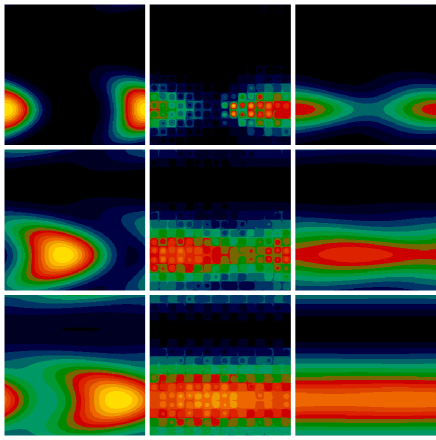
Figure 6: Snapshots of $\theta_{(M0)}$ (left column), $\theta_{(T)}$ (middle column), and $\theta_{(M2)}$ (right column) at three different time, from top to bottom $t\approx 0.5,1.0,1.5T$ where $T=L/U$ is the large scale advection time. The large-scale velocity field is the shear flow (26). At $t=0$ $\theta_{\alpha}$’s were initialized as a Gaussian centered in $(9/16L,7/16L)$ with a width $2\sigma\approx\ell$. Simulation parameters are summarized in table 1.

The improvement brought by the second-order corrections is even more striking if one looks directly to the snapshots of the concentrations fields (Figs. 6, 7). As one can see the spatial patterns of the M0 approximation rapidly decorrelate with those of the true field, that are actually well described by the M2 approximation. We remark crucial for the fidelity of the second-order approximation is that the corrections to the small-scale diffusivity tensor retains relevant information of the anisotropic and inhomogeneous diffusive behavior induced by the presence of the large-scale flow, namely the enhancement of diffusion in the direction on $\bm{U}$ and its reduction in the transverse direction. This is particularly evident in the case of large-scale shear shown in Fig. 6, where one can see that the blob M0 spreads too quickly in the $y$-direction and too slowly in the $x$-direction with respect to the true field. On the other hand, since $D^{(M2)}_{xx}>D^{(M0)}_{xx}$ and $D^{(M2)}_{yy}<D^{(M0)}_{yy}$ these features are captured by the M2 approximation. This is even clearer in Fig. 7, where one can see that, differently from the M2 model, the trapping of the concentration in the large-scale cells is completely missed in the M0 approximation.

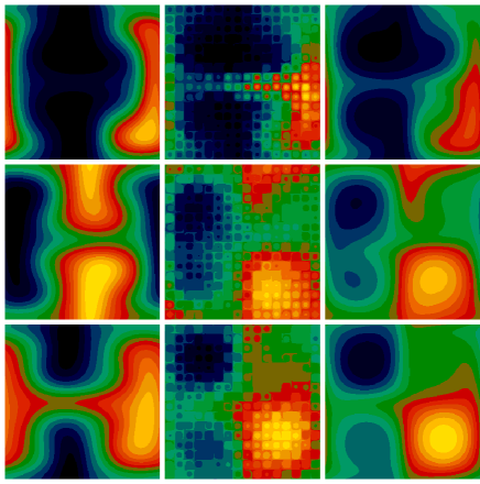
Figure 7: The same as in Fig. 6 for the case of large-scale cellular flow. Simulation parameters are summarized in table 1.

5 Conclusions

We have studied both analytically and numerically the effects of a weak advecting velocity field at large scale on the meso-scale modeling for the transport of passive scalars. By means of multiple-scale methods we perturbatively computed the dependence of (pre-asymptotic) eddy diffusion tensor $D_{ij}$ on the large-scale velocity field. The corrections to $D$ are non-homogeneous and non-isotropic. In particular we find an enhancement (reduction) in the longitudinal (transversal) direction of the large-scale field. The perturbative approach proposed here allows to develop meso-scale models retaining (at least at second order accuracy) these effects, which are shown to be crucial for properly describe the transport dynamics.

We conclude by noticing that the new findings obtained by our approach seem very promising for future applications to the numerical investigation of large-scale transport (asymptotic and pre-asymptotic) both in the atmosphere and in the ocean. Indeed the present results together with those obtained in Ref. [17] cover two opposite limit of transport for which explicit expressions for the effective parameters are available. By interpolations, one may hope to obtain the form of these effective coefficients under general conditions.

Appendix A Expressions for the asymptotic diffusivity

There are two, in principle non equivalent, ways to obtain the large-scale equation (29). The first one is to apply the homogenization technique to the exact equation (1), while the second possibility is to start from the meso-scale model equation (7). Following the first approach the (exact) value of the eddy-diffusivity tensor, $D^{{\mathcal{L}},ex}$, depends on both the molecular diffusivity and the advection by the total velocity field ${\bm{v}}={\bm{U}}+{\bm{u}}$:

$$D^{{\mathcal{L}},ex}_{ij}=D_{0}\delta_{ij}-\frac{\langle v_{i}\chi_{j}\rangle+\langle v_{j}\chi_{i}\rangle}{2}\;.$$ (32)

The auxiliary field ${\bm{\chi}}$ is the solution of the following equation

$$\partial_{t}{\bm{\chi}}+({\bm{v}}\cdot{\bm{\partial}}){\bm{\chi}}-D_{0}\partial^{2}{\bm{\chi}}=-{\bm{v}}\;.$$ (33)

With the second way the asymptotic eddy-diffusivity tensor $D^{\mathcal{L}}$ results from the combined effects of the advection given by the large-scale flow $\bm{U}({\bm{X}},T)$ and the effective diffusion at scale $\ell$ that depends on space and time through $D_{ij}({\bm{X}},T)$ (see [16] for a detailed derivation),

$$D^{\mathcal{L}}_{ij}=-\frac{\langle U_{i}\chi_{j}\rangle+\langle U_{j}\chi_{i}\rangle}{2}+\frac{\langle D_{ik}\partial_{k}\chi_{j}\rangle+\langle D_{jk}\partial_{k}\chi_{i}\rangle}{2}+\frac{\langle D_{ij}\rangle+\langle D_{ji}\rangle}{2}\,.$$ (34)

Here the vector field ${\bm{\chi}}$ is obtained by the auxiliary equation

$$\partial_{t}\chi_{k}+({\bm{U}}\cdot{\bm{\partial}})\chi_{k}-\partial_{i}(D_{ij}\partial_{j}\chi_{k})=-U_{k}+\partial_{i}D_{ik}\;.$$ (35)

It should be noted that even though the first procedure gives the exact value of the eddy-diffusivity tensor $D^{{\mathcal{L}},ex}$, it requires the detailed knowledge of the velocity field at both large and small scales. However, the expression obtained from Eq. (34) (which, in general, does not coincide with $D^{{\mathcal{L}},ex}$) has the advantage of being based solely on the large-scale velocity, $\bm{U}$, with the effects of the small-scale flow included in the eddy-diffusivity $D_{ij}({\bm{X}},T)$.

References

- [1] J.S. Martins J.B. Rundle M. Anghel, W. Klein, Phys. Rev. E 65, (2002) 056117.
- [2] D.L. Turcotte, Fractals and Chaos in Geology and Geophysics, (2nd ed., Cambridge Univ. Press, New York, 1997).
- [3] T. Murtola, E. Falck, M. Patra, M. Karttunen, and I. Vattulainen, J. Chem. Phys. 121, (2004) 9156.
- [4] J.M. Ottino, The Kinematics of Mixing: Stretching, Chaos and Transport, (Cambridge Univ. Press, New York, 1989).
- [5] O. Metais and J. Ferziger New Tools in Turbulence Modelling: Les Houches School (Springer-Verlag, Berlin 1996)
- [6] A. J. Majda and P. R. Kramer. Phys. Rep. 314 (1999) 237.
- [7] R.B. Stull, An Introduction to Boundary Layer Meteorology, (Kluwer Academic Publications, 1988).
- [8] A. Bensoussan, J.-L. Lions and G. Papanicolaou, Asymptotic Analysis for Periodic Structures (North-Holland, Amsterdam, 1978).
- [9] D. Mc Laughlin, G.C. Papanicolaou and O. Pironneau, SIAM Journal of Appl. Math. 45 (1985) 780.
- [10] R. N. Bhattacharya, V. K. Gupta, and H. F. Walker, SIAM J. Appl. Math. 49 (1989) 86.
- [11] L. Biferale, A. Crisanti, M. Vergassola and A. Vulpiani, Phys. Fluids 7 (1995) 2725 .
- [12] M. Vergassola and M. Avellaneda, Physica D 106 (1997) 148.
- [13] G. A. Pavliotis and P.R. Kramer, “Homogenized transport by a spatiotemporal mean flow with small-scale periodic fluctuations”, in proc. of the IV international conference on dynamical systems and differential equations, pp. 1-8, May 24 - 27, 2002, Wilmington, NC, USA.
- [14] R. Mauri, Phys. Rev. E 68 (2003) 066306.
- [15] A.S. Monin, and A. M. Yaglom, Statistical fluid mechanics (vol. II, MIT, Press, Cambridge, 1975).
- [16] A. Mazzino, Phys. Rev. E 56 (1997) 5500.
- [17] A. Mazzino, S. Musacchio and A. Vulpiani, Phys. Rev. E 71 (2005) 011113.
- [18] E.N. Lorenz, “Predictability - a problem partly solved” Proc. Seminar on predictability, Reading, U.K., European Centre for Medium-Range Weather Forecast, (1996) 1-18.
- [19] G. Boffetta, M. Cencini, M. Falcioni and A. Vulpiani, Phys. Rep. 356 (2002) 367.
- [20] P. Haynes and E. Shuckburgh, J. Geophys. Res, 105 (2000) 22777.
- [21] J. Marshall, E. Shuckburgh, H. Jones and C. Hill, (submitted to J. Phys. Oceanog.)
- [22] L. Meshalkin and Ya G. Sinai, J. Appl. Math. Mech. 25, (1961) 1700.
- [23] T.H. Solomon and J.P. Gollub Phys. Rev. A 38 (1988) 6280.
- [24] B. Y. Pomeau, C.R. Acad. Sci. Paris 301 (1985) 1323.
- [25] B.I. Shraiman, Phys. Rev. A 36 (1987) 261.