Discrete Solitons and Vortices on Anisotropic Lattices

Abstract

We consider effects of anisotropy on solitons of various types in two-dimensional nonlinear lattices, using the discrete nonlinear Schrödinger equation as a paradigm model. For fundamental solitons, we develop a variational approximation, which predicts that broad quasi-continuum solitons are unstable, while their strongly anisotropic counterparts are stable. By means of numerical methods, it is found that, in the general case, the fundamental solitons and simplest on-site-centered vortex solitons (“vortex crosses”) feature enhanced or reduced stability areas, depending on the strength of the anisotropy. More surprising is the effect of anisotropy on the so-called “super-symmetric” intersite-centered vortices (“vortex squares”), with the topological charge $S$ equal to the square’s size $M$: we predict in an analytical form by means of the Lyapunov-Schmidt theory, and confirm by numerical results, that arbitrarily weak anisotropy results in dramatic changes in the stability and dynamics in comparison with the degenerate, in this case, isotropic limit.

I Introduction and the model

In the last two decades, nonlinear lattice (spatially discrete) systems have been a very rapidly growing area of interest for a variety of applications reviews . Such systems arise in physical contexts encompassing, inter alia, beam dynamics in coupled waveguide arrays in nonlinear optics reviews1 , the time evolution of fragmented Bose-Einstein condensates (BECs) trapped in optical lattices (OLs) reviews2 , coupled cantilever systems in nano-mechanics sievers , denaturation of the DNA double strand in biophysics reviews3 and even stellar dynamics in astrophysics voglis .

One of the main objectives of the research in this field is to achieve an understanding of intrinsically localized states (discrete solitons). In two-dimensional (2D) lattices, these are fundamental discrete solitons solit and discrete vortices (i.e., localized states with an embedded nonzero phase circulation over a closed lattice contour) vort1 ; vort2 . Most recently, a substantial effort was dedicated to the experimental creation of both these entities in photonic lattices induced in photorefractive crystals (although these systems are only quasi-discrete). In particular, fundamental and dipole solitons, soliton trains and necklaces, and vector solitons have been reported esolit , as well as vortex solitons evort . Parallel developments in the experimental studies of soliton patterns in BECs have also been very substantial, leading to the creation of quasi-1D dark becd , bright becb and gap becg solitons. The generation of 2D BEC solitons in OLs has been theoretically demonstrated boris to be feasible with the currently available experimental technology old2d .

A paradigm dynamical lattice model that appears in the above-mentioned physical problems is the discrete nonlinear Schrödinger (DNLS) equation. Various applications of the DNLS equation are well documented reviews ; reviews1 ; reviews2 . Besides being a generic asymptotic form of a whole class of lattice models (for small-amplitude nonlinear excitations), it finds direct applications (where it furnishes extremely accurate description of the underlying physics) in terms of arrayed (1D) or bunched (2D) nonlinear optical waveguides, BECs trapped in strong OLs, and crystals built of optical or exciton microcavities.

An interesting issue in this framework that has not received sufficient attention concerns the influence of anisotropy on the soliton dynamics in 2D lattices. Some of the settings mentioned above are inherently anisotropic, e.g., photorefractive crystals solit ; esolit , while others (in particular, the fragmented BECs trapped in strong OLs reviews2 ) can be easily rendered anisotropic by slight variations of control parameters, such as intensities of laser beams that create two sublattices which together constitute the 2D optical lattice.

The aim of this paper is to understand how the lattice anisotropy affects 2D discrete solitons in the DNLS equation. Some findings reported below are surprising, demonstrating that anisotropy effects are not straightforward. The straightforward expectation might be that weak anisotropy is a small perturbation that possibly alters details of parametric dependences of the observed phenomenology but does not change it “structurally” (i.e., essentially the same dynamical features as in the isotropic lattice occur, but at different positions in the parameter space). We find that for the simplest soliton and vortex structures this is indeed the case, while for more sophisticated ones it is not. More specifically, we find that for especially symmetric (so-called “supersymmetric”) vortices, with their center set at an intersite position, and the topological charge equal to the size of the vortex square frame (see below for details), the isotropic lattice is a degenerate one, therefore even very weak anisotropy fundamentally alters the stability and dynamical properties of such structures. On the other hand, despite the delicate organization of the supersymmetric vortices, they constitute a structurally stable, i.e., physically meaningful, class of objects.

We take the DNLS equation in the following form:

$$i\dot{u}_{n,m}=-\epsilon\Delta_{\alpha}u_{n,m}-|u_{n,m}|^{2}u_{n,m},$$ (1)

where $u_{n,m}(t)$ is the complex, 2D lattice field (the overdot stands for its time derivative), $\epsilon$ is the lattice coupling constant, and

$$\begin{array}[]{rl}\Delta_{\alpha}u_{n,m}=&\alpha\left(u_{n+1,m}+u_{n-1,m}\right)+u_{n,m+1}\\[8.61108pt] &+u_{n,m-1}-2(1+\alpha)u_{n,m},\end{array}$$ (2)

is the anisotropic discrete Laplacian, which becomes isotropic with $\alpha=1$. Note that, unlike the continuum limit, no scaling transformation can cast the anisotropic DNLS equation into the isotropic form. Equation (1) conserves two dynamical invariants: the Hamiltonian,

$$\begin{array}[]{rcl}H&=&\sum_{n,m}\left[\left(u_{n,m+1}^{\ast}u_{n,m}+u_{n,m+1}u_{n,m}^{\ast}\right)\right.\\[8.61108pt] &&\left.+\alpha\left(u_{n+1,m}^{\ast}u_{n,m}+u_{n+1,m}u_{n,m}^{\ast}\right)\right.\\[8.61108pt] &&\displaystyle-\left.\left(\frac{\Lambda}{\epsilon}-2-2\alpha\right)\left|u_{n,m}\right|^{2}+\frac{1}{2\epsilon}\left|u_{n,m}\right|^{4}\right],\end{array}$$ (3)

and norm,

$$N=\sum_{n,m}\left|u_{n,m}\right|^{2},$$ (4)

where $\Lambda$ is the frequency of the internal mode (equivalently the chemical potential in the context of BECs or the propagation constant in the context of optical waveguide arrays).

Stationary solutions to Eq. (1) will be sought as

$$u_{n,m}=u_{n,m}^{(0)}\exp(i\Lambda t),$$ (5)

which leads to a stationary finite-difference equation,

$$\Lambda u_{n,m}^{(0)}=\epsilon\Delta_{\alpha}u_{n,m}^{(0)}-\left|u_{n,m}^{(0)}\right|^{2}u_{n,m}^{(0)}$$ (6)

(generally speaking, the discrete functions $u_{n,m}^{(0)}$ may be complex). In the case of fundamental-soliton solutions, we will apply the variational approximation (VA) to the real version of Eq. (6), which is based on the fact that it can be derived from the Lagrangian,

$$\begin{array}[]{rl}L=&\displaystyle\sum_{n,m}\left[u_{n,m+1}u_{n,m}+\alpha u_{n+1,m}u_{n,m}-\phantom{\frac{A}{A}}\right.\\[17.22217pt] &\displaystyle\left.\left(\frac{\Lambda}{2\epsilon}-1-\alpha\right)u_{n,m}^{2}+\frac{1}{4\epsilon}u_{n,m}^{4}\right].\end{array}$$ (7)

After analyzing fundamental solitons by means of the VA, we will construct discrete solitons in the anisotropic model and will study their stability by means of numerical methods. For the numerical procedure, our starting point is always the anti-continuum (AC) limit corresponding to $\epsilon=0$ mackay , where configurations of interest can be constructed at will as appropriate combinations of on-site states, which are either $u_{n,m}=\sqrt{\Lambda}\exp(i\Lambda t)$ with $\Lambda>0$ at excited sites, and $u_{n,m}\equiv 0$ at non-excited ones, cf. Eqs. (5) and (6) for the general case, $\epsilon>0$. The stability of the solitons is then analyzed by linearizing Eq. (1) for perturbations around a stationary solution $u_{n,m}^{(0)}e^{i\Lambda t}$,

$$u_{n,m}=\left[u_{n,m}^{(0)}+\delta\cdot\left(a_{n,m}e^{\lambda t}+b_{n,m}e^{\lambda^{\ast}t}\right)\right]e^{i\Lambda t},$$ (8)

where $\delta$ is an infinitesimal perturbation amplitude of the perturbation, and $\lambda$ is its eigenvalue. The Hamiltonian nature of the system dictates that if $\lambda$ is an eigenvalue, then so also are $-\lambda$, $\lambda^{\ast}$ and $-\lambda^{\ast}$ (in the stable case, $\lambda$ is imaginary, hence this symmetry yields only two different eigenvalues, $\lambda$ and $-\lambda$). Clearly, the stationary solution is unstable if at least one pair of eigenvalues features nonvanishing real parts.

It is noteworthy that the instability against perturbations corresponding to purely real eigenvalues $\lambda$ in Eq. (8) can be predicted by the Vakhitov-Kolokolov (VK) criterion VK : a soliton family, characterized by the dependence $N(\Lambda)$ [recall $N$ is the solution’s norm defined by Eq. (4)], may be stable under the condition $dN/d\Lambda>0$, and is definitely unstable in the opposite case. In particular, this criterion (as well as the VA) was found to be very useful and quite reliable in the investigation of 2D solitons in the Gross-Pitaevskii equation for BECs in 2D and quasi-1D periodic OL potentials Bakhtiyor , and even in 2D quasi-periodic potentials (such as the Penrose tiling among others) Bakhtiyor2 .

Our study of different states in the anisotropic model and their properties is structured as follows. In Section II, we present the VA for fundamental solitons. In Section III, discrete solitons and vortex crosses with the topological charge $S=1$ are considered, which are only perturbatively (weakly) affected by the anisotropy. In the following two sections, we will define and consider special “super-symmetric” configurations, with $S=1$ and $S=2$, respectively, and compare them with simpler cases. Finally, in section VI we summarize findings and present our conclusions.

II Variational approximation for fundamental solitons

As was shown in Ref. MIW for the one-dimensional DNLS equation (see also Ref. MIW2 , for a more rigorous variational approach applied to higher dimensional solitons in the isotropic case), the only analytically tractable variational ansatz for stationary fundamental solitons may be based on the following cusp-shaped expression (in the 2D case, it has the shape of a cross cusp),

$$u_{n,m}^{(0)}=A\exp\left(-a|n|-b|m|\right),$$ (9)

with positive parameters $a$ and $b$, that determine the widths of the soliton in the horizontal and vertical directions, and an arbitrary amplitude $A$. Note that expression (9) is indeed an exact solution to the linearized version of Eq. (6), which describes soliton tails, if $\Lambda$ is linked to $a$ and $b$ by the dispersion relation,

$$\Lambda=2\epsilon\left[\alpha\sinh^{2}(a/2)+\sinh^{2}(b/2)\right].$$ (10)

The substitution of ansatz (9) makes it possible to calculate the corresponding effective Lagrangian explicitly. First of all, it is convenient to eliminate the amplitude in favor of the norm (4). Indeed, the substitution of the ansatz in the definition of $N$ yields $A^{2}=N\tanh a\cdot\tanh b$. After this, the effective Lagrangian becomes

$$L_{\mathrm{eff}} = N~{}\left(\alpha\mathrm{sech}a+\mathrm{sech}b\right)-\left(\frac{\Lambda}{2\epsilon}+1+\alpha\right)N$$ (11)

$$+ \frac{N^{2}}{16\epsilon}\frac{\cosh\left(2a\right)\cosh\left(2b\right)\sinh a\sinh b}{\cosh^{3}(a)\cosh^{3}(b)}~{}.$$

Variational equations for the stationary profile are obtained from here in the form

$$\frac{\partial L_{\mathrm{eff}}}{\partial N}=\frac{\partial L_{\mathrm{eff}}}{\partial a}=\frac{\partial L_{\mathrm{eff}}}{\partial b}=0.$$ (12)

In the general case, the explicit form of these equations is quite cumbersome (this will be treated numerically, see below). A detailed analysis is possible in two special cases, as specified below.

First is the case of small $a$ and $b$ ($a,b\ll 1$), which implies broad solitons. Then, the expansion of the effective Lagrangian (11) yields

$$L_{\mathrm{eff}} \approx -\frac{\Lambda}{2\epsilon}N+\frac{1}{2}N\left(-b^{2}-\alpha a^{2}+\frac{5}{12}b^{4}+\frac{5\alpha}{12}a^{4}\right)$$ (13)

$$+\frac{N^{4}}{16\epsilon}\left(ab+\frac{2}{3}a^{3}b+\frac{2}{3}ab^{3}\right),$$

and the variational equations (12) following from Eq. (13) generate the following solution:

$$N = 16\epsilon\sqrt{\alpha}\left(1-\frac{7}{8}\frac{\alpha+1}{\alpha}\frac{\Lambda}{\epsilon}\right),$$ (14)

$$a^{2} = \frac{\Lambda}{2\epsilon\alpha},~{}b=\sqrt{\alpha}a.$$ (15)

As follows from these expressions, the underlying assumptions $a,b\ll 1$ indeed hold (i.e., the approximation is self-consistent) under the condition

$$\Lambda\ll\left\{\begin{array}[]{cc}\alpha\epsilon,&\mathrm{if~{}}\alpha~\,{}_{\sim}^{>}~{}1,\\ \epsilon,&\mathrm{if~{}}\alpha\gg~{}1.\end{array}\right.$$ (16)

The broad (quasi-continuum) solitons predicted in this approximation are unstable according to the VK criterion, as Eq. (14) immediately shows that $dN/d\Lambda<0$.

Note that the expansion of the dispersion relation (10) for the same case of small $a$ and $b$ yields $\alpha a^{2}+b^{2}=\Lambda/\epsilon$. It is noteworthy that this relation, although derived independently of the variational equations, is consistent with Eq. (15).

Another tractable case is that of a strongly anisotropic soliton, which is broad (quasi-continuum) in either direction and narrow in the other, i.e., it corresponds to $a\ll 1,b\gg 1$, or vice versa. If $a$ is small and $b$ is large, the variational equations (12) yield the following results:

$$a=\sqrt{\frac{\Lambda}{3\alpha\epsilon}},~{}\sinh\left(\frac{b}{2}\right)=\sqrt{\frac{\Lambda}{\epsilon}},~{}N^{2}=\frac{4}{3}\epsilon\alpha\Lambda.$$ (17)

These results are consistent with the underlying assumptions ($a\ll 1,b\gg 1$) under the conditions

$$1\ll\Lambda/\epsilon\ll\alpha.$$ (18)

On the contrary to the broad solitons given above by Eqs. (14) and (15), Eqs. (17) show that the anisotropic solitons are stable as per the VK criterion, as they obviously meet the condition $dN/d\Lambda>0$.

For the opposite strongly anisotropic case, with $a\gg 1$ and $b\ll 1$, the result is

$$b=\sqrt{\frac{\Lambda}{3\epsilon}},~{}\sinh\left(\frac{a}{2}\right)=\sqrt{\frac{\Lambda}{\alpha\epsilon}},~{}N^{2}=\frac{4}{3}\epsilon\Lambda,$$ (19)

cf. Eqs. (17). These expressions comply with the underlying assumptions $a\gg 1,b\ll 1$ provided that

$$\alpha\ll\Lambda/\epsilon\ll 1,$$ (20)

cf. Eq. (18). Similarly to the solution of Eq. (17), the one of Eq. (19) obviously meets the VK stability criterion.

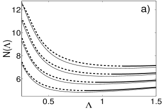
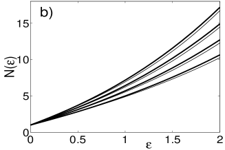
Figure 1: a) Norm of the solution vs. $\Lambda$ for several values of the anisotropy and fixed coupling strength $\epsilon=1$. For all the panels in this figure the anisotropy values are $\alpha=1.5,1.25,1,0.75$, respectively, for each curve from top to bottom. Thick lines (solid and dashed) represent direct numerical results and the thin lines represent the VA. The dashed lines correspond to unstable soliton solutions Note that the sign of the slope of $N(\Lambda)$ reflects the stability of the soliton solutions as predicted by the VK criterion. b) The norm of the soliton solution as a function of the coupling strength for fixed $\Lambda=1$. Once again, thick lines represent direct numerical results and thin lines illustrate the VA.

Lastly, inequalities (18) and (20) imply that the above solutions indeed pertain to the strongly anisotropic model, as the corresponding parameter $\alpha$ is large in the former case, and small in the latter one. We also notice that the condition (18) in the case of large $\alpha$, or its counterpart (20) in the opposite case of small $\alpha$, is incompatible with the respective condition (16), i.e. (as one would expect), the existence regions of the unstable quasi-continuum solitons and stable strongly anisotropic ones have no overlap.

For general $a$ and $b$, the variational equations (12), with the effective Lagrangian (11), cannot be solved explicitly and one has to find $(N,a,b)$ solutions numerically for each $(\epsilon,\Lambda)$ pair. In Fig. 1 we compare the results obtained from the VA with solutions obtained through numerically solving the stationary equation (5). Fig. 1.a depicts the norm of the soliton solutions as a function of the propagation constant $\Lambda$ for several values of the anisotropy parameter $\alpha$ and for constant coupling ($\epsilon=1$). As may be noticed from the figure, the VA (thin lines) provides a good approximation to the actual solution (thick lines). We also checked the stability of the constructed solutions by following the largest real eigenvalue (see also details below). of the linearized problem defined in Eq. (8). Stable solutions are depicted with solid lines while unstable solutions correspond to dashed lines. As is clear from the figure, the slope of $N(\Lambda)$ predicts the stability of the solution according to the VK criterion (see above). Furthermore, since the VA gives a good approximation of $N(\Lambda)$, it is possible to obtain a good estimate for the transition from stable to unstable solutions, as $\Lambda$ is decreased, using the VA together with the VK criterion. Finally, in Fig. 1.b we fix $\Lambda=1$ and perform a similar calculation by varying the coupling strength $\epsilon$. Again, the VA (thin lines) approximates remarkably well the norm of the solutions (thick lines).

III Fundamental solitons and vortex crosses: numerical results

We start numerical computations with a single excited site in the AC limit, and continue the solution in $\epsilon$ (for a fixed value of the anisotropy parameter $\alpha$). The objective is to construct regular site-centered discrete solitons, with the anticipation that, as is known for the isotropic model ($\alpha=1$), the solitons will be stable up to a critical value of the coupling constant, i.e., at $\epsilon<\epsilon_{\mathrm{cr}}$ MIW2 ; 2d . At $\epsilon>\epsilon_{\mathrm{cr}}$, the discrete solitons are found to be unstable due to a real eigenvalue arising in the linearization around the soliton. In the numerical part of the work (unlike the VA considered above), we fix $\Lambda=1$ in Eq. (6), using the scaling invariance of Eq. (1), and examine how $\epsilon_{\mathrm{cr}}$ is affected by the variation of $\alpha$. The results will be summarized in the form of two-parameter diagrams that chart regions of stable and unstable discrete states.

For regular discrete solitons, such a diagram is presented in Fig. 2. The top panel illustrates the fact that the increase of $\alpha$ gradually destabilizes the solitons, i.e., $\epsilon_{\mathrm{cr}}$ decreases with increasing $\alpha$. Interestingly, the respective dependence is very well approximated by an empirical relation $\epsilon_{\mathrm{cr}}=1/\sqrt{\alpha}$. More accurately, the best fit to this numerical dependence is given by: $\epsilon_{\mathrm{cr}}\approx 0.999\alpha^{-0.488}$. The middle panel in Fig. 2 illustrates in more detail some special cases of this dependence for $\alpha=1$ (solid lines), $\alpha=1.25$ (dashed lines) and $\alpha=0.75$ (dash-dotted lines).

We note that, in terms of the general equation (1), the cases of $\alpha<1$ and $\alpha>1$ are tantamount to each other, as one may divide the equation by $\alpha$, mutually rename the vertical and horizontal indices ($n$ and $m$), and then rescale the equation to the form with $\alpha$ replaced by $1/\alpha$. However, this transformation is not possible once we fix $\Lambda\equiv 1$, which is why we report results below for both $\alpha>1$ and $\alpha<1$.

For $\alpha=1$, an eigenvalue bifurcates from the edge of the continuous spectrum at $\epsilon\approx 0.445$, and with further increase of $\epsilon$ it moves towards the origin of the spectral plane $(\lambda_{r},\lambda_{i})$ (the subscripts denote the real and imaginary part of the eigenvalue) . It becomes unstable, reaching the origin at $\epsilon\approx 1.006$. For $\alpha=1.25$, the first bifurcation occurs at $\epsilon\approx 0.398,$ and the instability sets in at $\epsilon\approx 0.896$, whereas for $\alpha=0.75$ the respective critical points (the appearance of the eigenvalue, and its passage into the instability region) are found at $\epsilon\approx 0.511$ and $1.156$, respectively. Notice that these results are quite natural since, as $\alpha\rightarrow 0$, the system becomes nearly one-dimensional, hence we expect the destabilization point to approach its 1D counterpart. Thus, as the 1D discrete solitons are well-known to be stable up to the continuum limit, one may expect that $\epsilon_{\mathrm{cr}}\rightarrow\infty$ for $\alpha\rightarrow 0$. The bottom panel of Fig. 2 shows an example of a discrete soliton for $\alpha=1.5$ and $\epsilon=1$. Although the anisotropy is hardly observed in this case, it can be traced nevertheless; in particular, $u_{1,0}=0.785$, and $u_{0,1}=0.579$.

  

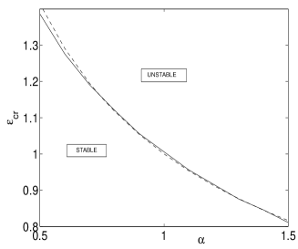
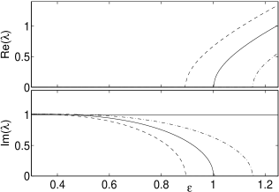
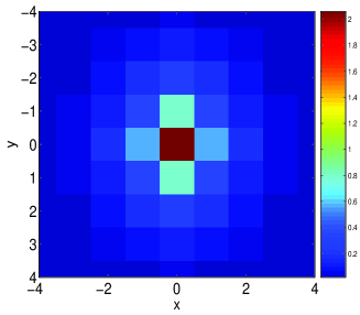
Figure 2: The soliton line in the top panel shows the critical value of $\epsilon$ (the border between stable and unstable discrete solitons) as a function of $\alpha$; the dashed line is $\epsilon=1/\sqrt{\alpha}$. The middle panel shows how the real and imaginary parts of the stability eigenvalue, $\lambda_{r}$ and $\lambda_{i}$, depend on $\epsilon$ for $\alpha=1.25,~{}1$, and $0.75$ (dashed, solid, and dash-dotted curves, respectively). The bottom panel shows an example of the discrete soliton found for $\epsilon=1$ and $\alpha=1.5$.

Similar results can be obtained for on-site vortices (discrete vortex solitons) with the topological charge $S=1$. In this section, we consider the solitons in the form of the so-called “vortex cross”, with $u_{1,0}=1$, $u_{0,1}=\exp(i\pi/2)\equiv i$, $u_{-1,0}=\exp(i\pi)\equiv-1$, $u_{0,-1}=\exp(i3\pi/2)\equiv-i$ (and $u_{0,0}=0$, at the central point), excited in the AC limit vort1 . There are interesting variations to this problem, in comparison with the fundamental soliton. In particular, the respective instability mechanism is different, as it is caused by an eigenvalue bifurcating from the origin in the spectral plane for $\epsilon\neq 0$, and eventually (upon parametric continuation) colliding with the edge of the continuous spectrum (or an eigenvalue bifurcating from the continuous spectrum). The collision gives rise to a quartet of eigenvalues, through the so-called Hamiltonian-Hopf bifurcation hamilton . In the isotropic case ($\alpha=1$), it is known that this instability sets in at $\epsilon_{\mathrm{cr}}\approx 0.39$ vort1 , while, in the present anisotropic model, we have found that $\epsilon_{\mathrm{cr}}\approx 0.325$ for $\alpha=1.3$ and $\epsilon_{\mathrm{cr}}\approx 0.429$ for $\alpha=0.7$. The respective two-parameter diagram $(\epsilon_{\mathrm{cr}},a)$ is shown in the top panel of Fig. 3. The cases of $\alpha=1.3$, $1$, and $0.7$ (dashed, solid and dash-dotted, dashed-dotted curves, respectively) are shown in the middle panel. The bottom panel of the figure illustrates the squared-amplitude profile of the discrete vortex for $\alpha=0.2$ and $\epsilon=0.5$. The sites $(1,0)$ and $(0,1)$ have the squared amplitudes $|u_{1,0}|^{2}=1.934$ and $|u_{0,1}|^{2}=2.057$, respectively. Notice also that as $\alpha\rightarrow 0$, a quasi-1D situation is again approached, where the so-called twisted-localized mode (TLM) TLM configuration (alias an odd soliton) is a counterpart of the 2D vortex. As one would expect, the critical point of the instability departs from the value $\epsilon_{\mathrm{cr}}^{(\mathrm{2D})}\approx 0.39$, corresponding to the isotropic 2D case, towards the value corresponding to the stability border of the 1D TLM solitons, which is $\epsilon_{\mathrm{cr}}^{(\mathrm{1D})}\approx 0.433$.

  

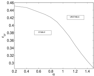
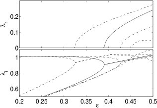
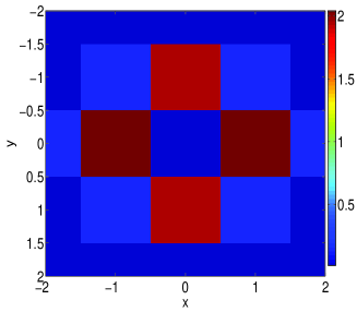
Figure 3: The top panel shows the critical value of $\epsilon$ separating the stable and unstable discrete vortices (on-site-centered ones, alias vortex crosses) with $S=1$ as a function of $\alpha$. The middle panel shows how the real and imaginary parts of the eigenvalue leading to the instability depend on $\epsilon$ for $\alpha=1.3,~{}1$, and $0.7$ (dashed, solid and dash-dotted curves, respectively). Notice that, for $\alpha=1.3$, there is a secondary instability arising for $\epsilon>0.433$. The bottom panel shows the squared-absolute-value profile of the discrete vortex for $\epsilon=0.5$ and $\alpha=0.2$.

IV Fundamental vortex squares

For the discrete solitons examined so far, the difference between the isotropic and non-isotropic cases has not been particularly dramatic; the anisotropy chiefly entailed a smooth deformation of the instability-onset scenarios known for the isotropic case. Therefore, the dynamical evolution triggered by the instability is naturally expected to be similar to that in previously studied isotropic cases solit ; vort1 ; vort2 ; 2d .

Now we will give an example where the instability scenario and dynamics are very different from their isotropic counterparts. We focus, in particular, on the off site-centered vortex (alias “vortex square”) vort1 ; vort2 . The vortex-square contours are characterized by their size $M$, which is the number of lattice bonds that each side of the square contour contains in the AC-limit pattern, from which the solution family stems. Hence, the vortex square based, in the AC limit, on the set of sites $(0,0),(1,0),(1,1),(0,1)$ is the $M=1$ contour. The configuration with $S=1$ is written on this set by lending the four sites the phases $0$, $\pi/2$, $\pi$ and $3\pi/2$, respectively. The persistence of such configurations, as was discussed in detail in Ref. dep , is determined by whether secular conditions (obtained from the Lyapunov-Schmidt theory golub ), excluding the projection of eigenvectors in the kernel of the linearization at $\epsilon=0$ to the solution at finite $\epsilon$, are satisfied. In the isotropic case, to leading order ($O$($\epsilon$)), these secular conditions are found to be

$$0=f(\theta_{l})\equiv\sin(\theta_{l}-\theta_{l+1})+\sin(\theta_{l}-\theta_{l-1})$$ (21)

for $l=1,\dots,N$ (with periodic boundary conditions), where $N=4M$ is the number of sites participating in the contour and $\theta_{l}$ are their respective phases [cf. Eqs. (3.1)–(3.2) of Ref. dep ].

One can then apply similar arguments to the present setting and derive modified persistence criteria for the anisotropic model. For $M=1$, they are

$$0=f(\theta_{l})\equiv\left\{\begin{array}[]{rcl}\alpha\sin(\theta_{l}-\theta_{l+1})&+&\sin(\theta_{l}-\theta_{l-1})\\[2.15277pt] l&=&2k+1,k=0,1\\[8.61108pt] \sin(\theta_{l}-\theta_{l+1})&+&\alpha\sin(\theta_{l}-\theta_{l-1})\\[2.15277pt] l&=&2k,k=1,2.\end{array}\right.$$ (22)

While Eqs. (22) may seem a moderate modification of (21), there is a crucial (for stability purposes) difference. Indeed, consider the linearization around the $S=1$ solution according to Eq. (8). It was proved in Ref. dep that the Jacobian matrix of the reduced set of Eqs. (22), defined through $J_{lk}=\partial f_{l}/\partial\theta_{k}$, determines leading-order corrections to $N-1$ eigenvalue pairs bifurcating from the origin [one pair stays at the origin due to the invariance of Eq. (1) with respect to the phase shift], since these eigenvalues satisfy the equation:

$$\lambda_{l}^{2}=2\epsilon\mu_{l},$$ (23)

with $\mu_{l}$ the corresponding eigenvalues of the reduced $N\times N$ Jacobian $J_{lk}$. It is further easy to check that, for the vortex square with $S=1$ and $M=1$, the entire Jacobian matrix consists of zeros. More generally, as shown in Ref. dep , this is the case for the square vortices of size $M$ with charge $S=M$, which for that reason were termed “super-symmetric” vortices. Obviously, to determine the stability of the vortices in this special case, one needs to go to higher-order expansions. Typically, second-order reductions will yield a non-trivial result for the stability of such super-symmetric configurations, leading to eigenvalue dependences $\lambda_{l}\propto\epsilon$ [rather than $\lambda_{j}\propto\sqrt{\epsilon}$, as dictated by Eq. (23) in the generic case].

The key variation to this theme stemming from the presence of the anisotropy is that the matrix $J_{lk}$ has generically non-vanishing elements in the lowest approximation for $\alpha\neq 1$; in other words, the isotropic lattice is a degenerate one for the supersymmetric solitons, and arbitrarily weak anisotropy lifts this degeneracy. As a result, the eigenvalue bifurcations occur, typically, at the leading order, rather than at the second-order perturbation expansions, which was the case in the isotropic model. More strikingly, considering a specific example, such as for $\alpha=1.05$ (a very weak deviation from the isotropic case), we find that the relevant angles (in radians) satisfying the conditions (22) are $\theta_{1}=-0.0229$, $\theta_{2}=1.8577$, $\theta_{3}=3.4285$, and $\theta_{4}=4.6895$; the corresponding $4\times 4$ Jacobian has two zero eigenvalues (one of which will split to order $O(\epsilon)$, see below) and two nonzero ones, $\pm 0.6403$. From the existence of the positive eigenvalue and from Eq. (23), it immediately follows that the $S=M=1$ configuration is immediately unstable (for all values of $\epsilon$). This is in complete contrast with the super-symmetric vortex in the isotropic model, which has two imaginary eigenvalue pairs (bifurcating at the second-order reduction), $\lambda\approx\pm 2i\epsilon$, and is linearly stable for $\epsilon<\epsilon_{c}\approx 0.38$.

From here, we conclude that the anisotropy can play a critical role in destabilizing configurations that would be very robust ones in the isotropic limit. Furthermore, this can happen arbitrarily close to the isotropic limit (that turns out to be a very delicate one), given the nature of the argument presented above. We also note in passing that in the anisotropic case examined above, there is yet another real eigenvalue pair which is $\lambda\approx\pm 3\epsilon$ for small $\epsilon$ (this pair stems from the higher-order reduction, in agreement with the prediction of the reduced Jacobian). These two eigenvalue pairs eventually collide at $\epsilon=0.057$, resulting in a Hamiltonian Hopf bifurcation to an eigenvalue quartet which is present in the stability spectrum at $\epsilon>0.057$. This phenomenology is shown in Fig. 4. The leading-order prediction for the most unstable eigenvalue is in good agreement with the full numerical result for small values of $\epsilon$. For higher values of $\epsilon$, the second-order corrections that we do not examine here in detail come into play and lead to the Hamiltonian Hopf bifurcation.

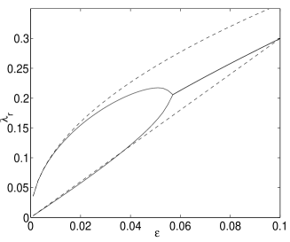
Figure 4: For the $S=1$ super-symmetric square vortex (one with the size $M=1$), two real stability eigenvalues are shown as functions of $\epsilon$ for $\alpha=1.05$. The numerical and analytical results (see text) are displayed, respectively, by the solid lines and dashed lines.

To directly compare the dynamics between the isotropic and weakly anisotropic (yet unstable) case for the super-symmetric vortex, we have performed numerical simulations. Detailed simulations are reported in this work only for the super-symmetric cases (see also the next section), since for all other states anisotropy operates as a regular perturbation, see above; as a result, instabilities of the other states may be shifted due to the anisotropy, but structurally the phenomenology remains the same.

For the delicate super-symmetric vortex square, the dynamics altered by the anisotropy is indeed found to be dramatically different from the isotropic case. This is illustrated by Fig. 5, for the vortex square with $S=M=1$, carried (in the AC limit) by $4$ sites. The time dynamics of the squared absolute value of the field at the main sites is shown in the figure for a weakly anisotropic model, with $\alpha=1.05$, and its isotropic counterpart (top and bottom panels, respectively). Stark contrast between the instability developing for $t>50$ in the former case, versus the complete stability for all times in the latter (isotropic) system, is obvious (notice the difference in the scales of vertical axes between the two panels). In the linear approximation, these results are well predicted by the above theory.

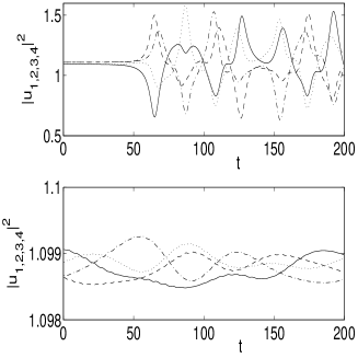
Figure 5: The dynamics of an initially very weakly perturbed super-symmetric vortex with $S=M=1$, principally based on four lattice sites that form an elementary cell (the sites are labeled as $1,2,3,4$). The time evolution of the squared absolute value of the fields at these sites is shown in the top panel for a weakly anisotropic model, with $\alpha=1.05$, and for its isotropic counterpart ($\alpha=1$) in the bottom panel. In both cases, the same uniformly distributed, random initial perturbation of amplitude $10^{-4}$ was added to the solution at $t=0$ to excite possible instabilities. Clearly, the vortex on the weakly anisotropic lattice becomes unstable at $t>50$, while in the isotropic case the perturbation remains bounded and small at all times. In these examples, the intersite lattice coupling constant is $\epsilon=0.025$.

V Higher-order vortices

We now give a summary of results for vortices with higher values of the topological charge. First, we consider the $S=M=2$ super-symmetric vortex populating the sites $(1,0)$, $(1,1)$, $(0,1)$, $(-1,1)$, $(-1,0)$, $(-1,-1)$, $(0,-1)$, $(1,-1)$ in the AC limit, with a phase shift of $\pi/2$ between adjacent sites (in the isotropic model). The latter provides for a total phase gain of $4\pi$ around a closed path surrounding the origin. This type of the configuration with $S=M=2$ was identified in Ref. dep as possessing a real eigenvalue pair with $\lambda_{r}=\pm\sqrt{\sqrt{80}-8}\epsilon$, in excellent agreement with numerical computations. However, the presence of the small anisotropy for $\alpha\neq 1$ again strongly affects the vortex for reasons similar to the ones presented above. In this case, the reductions leading to the perturbed dynamics in the anisotropic model are described by the following persistence conditions:

$$0=f(\theta_{l})\equiv\left\{\begin{array}[]{rcl}\sin(\theta_{l}-\theta_{l+1})&+&\sin(\theta_{l}-\theta_{l-1})\\[2.15277pt] i&=&2k+1,k=0,1,2,3,\\[8.61108pt] \alpha\sin(\theta_{l}-\theta_{l+1})&+&\sin(\theta_{l}-\theta_{l-1})\\[2.15277pt] i&=&4k+2,k=0,1,\\[8.61108pt] \sin(\theta_{l}-\theta_{l+1})&+&\alpha\sin(\theta_{l}-\theta_{l-1})\\[2.15277pt] i&=&4k+4,k=0,1,\end{array}\right.$$ (24)

cf. Eqs. (22). In this expression $\theta_{l}$ is the phase of the field at each of the eight above-mentioned sites (where, in the order the sites were mentioned, the corresponding index is $l=1,2,\dots,8$). Furthermore, as discussed above, the analysis performed in Ref. dep can be used to show that the linear stability eigenvalues for such a vortex soliton will be given, to the leading order, by Eq. (23). Using this prediction, even in the weakly anisotropic case (e.g., for $\alpha=1.05$) one finds that the corresponding $8\times 8$ Jacobian possesses three real $O(\sqrt{\epsilon})$ eigenvalues, which result in an instability (contrary to the single real $O(\epsilon)$ eigenvalue in the $\alpha=1$ case). Hence, once again, the anisotropy results in a significant destabilization of the super-symmetric vortex, in comparison to the isotropic model. As a specific example, we show in Fig. 6) the situation for $\alpha=1.05$. The solution of Eqs. (24) yields $\theta_{1}=0.218$, $\theta_{2}=1.967$, $\theta_{3}=3.182$, $\theta_{4}=4.397$, $\theta_{5}=6.145$, $\theta_{6}=7.894$, $\theta_{7}=9.109$, $\theta_{8}=11.036$, which, in turn, results in a Jacobian with the 3 real eigenvalues $\mu=\{1.0145,0.5357,0.2391\}$. The comparison of the numerical prediction for the eigenvalue dependence on $\epsilon$ versus the corresponding analytical prediction (solid and dashed lines, respectively) based on the above results is given in Fig. 6, demonstrating a very good agreement between the two.

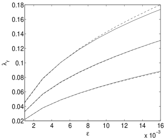
Figure 6: For the $S=M=2$ supersymmetric vortex, the three real eigenvalues are displayed as functions of $\epsilon$ for $\alpha=1.05$. The solid and dashed lines depict the numerical and analytical results.

To highlight the substantial differences between the dynamics in the isotropic and anisotropic models, we have performed numerical simulations of the super-symmetric vortex with $S=M=2$. In this case, the evolution of the field at the eight basic sites is shown in the top panel of Fig. 7 for $\alpha=1.05$, and in the bottom panel for $\alpha=1$. In the former case, for the coupling strength $\epsilon=0.015$ considered here, the three unstable eigenvalues for $\alpha=1.05$ are $\lambda=0.1688$, $\lambda=0.1258$ and $\lambda=0.0855$, while in the latter case (isotropic model), the only unstable eigenvalue is a much smaller one, $\lambda=0.0146$. Naturally, we observe the instability setting in much earlier in the anisotropic model (at $t~\,{}_{\sim}^{>}~{}30$) than in the isotropic one (at $t~\,{}_{\sim}^{>}~{}160$).

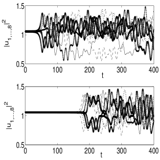
Figure 7: Same as in Fig. 5 but for the supersymmetric vortex of the $S=M=2$ type. The four lines (solid, dashed, dotted, and dash-dotted) and four symbols (circles, pluses, stars and triangles) are used to denote the squared absolute values of the field at the eight sites carrying the vortex in the anisotropic (top) model and its isotropic counterpart (bottom) for $\epsilon=0.015$.

One may be wondering whether the strong dynamical effect of the weak anisotropy should be attributed to the super-symmetry of the vortex, or maybe just the specific type of contour which carries the vortex. To check this, we have also considered the vortex with $S=3$ sitting on the same $M=2$ contour. Given the lack of the super-symmetry in the latter case, the bifurcation of the relevant $7$ ($=N-1$) eigenvalue pairs occurs at the leading-order reduction and all of them are proportional to $\pm i\sqrt{\epsilon}$. More specifically, for the largest pair in the isotropic case (for instance), the proportionality factor is $2.3784$. In the anisotropic case with $\alpha=1.05$, the seven pairs remain on the imaginary axis, being slightly perturbed due to $\alpha\neq 1$. For instance, the largest one among them is now $\lambda=\pm 2.3943\cdot i\sqrt{\epsilon}$. On the other hand, for $\alpha=0.95$, the largest eigenvalue pair is $\lambda=\pm 2.3647\cdot i\sqrt{\epsilon}$. This also is in line with our above results on the fundamental discrete soliton and vortex cross, since it indicates that, for $\alpha>1$, the collision of this eigenvalue with the continuous spectrum (which leads to the Hamiltonian Hopf bifurcation) will occur at smaller $\epsilon$, the opposite being true for $\alpha<1$. Hence the stability diagram of the $S=3,M=2$ vortex square is quite similar to that shown for the fundamental soliton and vortex cross in Figs. 2 and 3 (therefore, it is not shown here).

VI Conclusions

In this work, we have examined effects of anisotropy on lattice nonlinear dynamical systems supporting discrete solitons and vortices. The two-dimensional discrete nonlinear Schrödinger equation was used as a paradigm model. The variational approximation was developed for fundamental solitons, showing (by means of the Vakhitov-Kolokolov criterion) that broad quasi-continuum ones are unstable, while strongly anisotropic solitons are stable. By means of numerical methods, we have found that usual localized states, such as the fundamental discrete solitons and vortex crosses, are only mildly affected by the anisotropy, which results in a modified stability region (reduced when one direction features a stronger coupling than the isotropic limit, and augmented when the coupling along this direction is weaker). General phenomenology for such states is similar to that for their counterparts on the isotropic lattice.

The main finding reported in the present work is that the assumption about mild deformation of the stability region induced by weak anisotropy is not valid for the delicate super-symmetric vortex states residing on square contours, in the case when the vorticity $S$ is equal to the contour’s size $M$. In this special case, the degeneracy of the leading-order existence conditions (dictated by Lyapunov-Schmidt theory) specific to the isotropic case is broken by the anisotropy. This, in turn, results in a dramatically different behavior (as a function of the intersite coupling constant) of the corresponding linear stability eigenvalues, in terms of both the order of their bifurcation, and the number of real eigenvalues. As a consequence, the supersymmetric vortex-square structure that was marginally stable in the isotropic case is found to be strongly unstable even on the weakly anisotropic lattice. Similarly, the supersymmetric vortex with $S=M=2$ is found to be much more unstable in the anisotropic case in comparison to its isotropic counterpart.

The most natural systems for experimental observation of the results predicted in this work are deep optical lattices trapping BECs, and bundled sets of nonlinear optical waveguides (the latter have been recently created experimentally Lederer ). Anisotropic lattices can also be induced in photorefractive media, but this medium should be considered separately, in view of the different (saturable) character of the optical nonlinearity in this case. Such investigations are currently in progress and will be reported elsewhere.

A further natural extension of this work would be to examine effects of anisotropy in three-dimensional lattices on discrete solitons, vortices, dipoles and quadrupoles of various types, octupoles, and more exotic localized configurations, that were recently investigated for the isotropic case in Refs. vortex3d .

References

- (1) S. Aubry, Physica D 103, 201, (1997); S. Flach and C. R. Willis, Phys. Rep. 295 181 (1998); D. Hennig and G. Tsironis, Phys. Rep. 307, 333 (1999); P. G. Kevrekidis, K. Ø. Rasmussen, and A. R. Bishop, Int. J. Mod. Phys. B 15, 2833 (2001).
- (2) D. N. Christodoulides, F. Lederer and Y. Silberberg, Nature 424, 817 (2003); Yu. S. Kivshar and G. P. Agrawal, Optical Solitons: From Fibers to Photonic Crystals, Academic Press (San Diego, CA, 2003).
- (3) P. G. Kevrekidis and D. J. Frantzeskakis, Mod. Phys. Lett. B 18, 173 (2004); V. V. Konotop and V. A. Brazhnyi, Mod. Phys. Lett. B 18 627, (2004); P. G. Kevrekidis, R. Carretero-González, D. J. Frantzeskakis, and I. G. Kevrekidis, Mod. Phys. Lett. B 18, 1481 (2004).
- (4) M. Sato and A. J. Sievers, Nature 432, 486 (2004); M. Sato, B. E. Hubbard, A. J. Sievers, B. Ilic and H. G. Craighead, Europhys. Lett. 66, 318 (2004); M. Sato, B. E. Hubbard, A. J. Sievers, B. Ilic, D. A. Czaplewski, and H. G. Craighead, Phys. Rev. Lett. 90, 044102 (2003).
- (5) M. Peyrard, Nonlinearity 17, R1 (2004).
- (6) N. Voglis, Mon. Not. Roy. Astr. Soc. 344, 575 (2003).
- (7) N. K. Efremidis, et al., S. Sears, D. N. Christodoulides, J. W. Fleischer, and M. Segev, Phys. Rev. E 66, 046602 (2002); A. A. Sukhorukov, Yu. S. Kivshar, H. S Eisenberg, and Y. Silberberg, IEEE J. Quantum Electron. 39, 31 (2003).
- (8) B. A. Malomed and P. G. Kevrekidis, Phys. Rev. E 64, 026601 (2001).
- (9) J. Yang and Z. Musslimani, Opt. Lett. 23, 2094 (2003), P. G. Kevrekidis, B. A. Malomed, Z. G. Chen, and D. J. Frantzeskakis, Phys. Rev. E 70, 056612 (2004).
- (10) J. W. Fleischer, T. Carmon, M. Segev, N. K. Efremidis, and D. N Christodoulides, Phys. Rev. Lett. 90 023902 (2003); H. Martin, E. D. Eugenieva, Z. G. Chen, and D. N. Christodoulides, Phys. Rev. Lett. 92 123902 (2004); J. K Yang, I. Makasyuk, A. Bezryadina, and Z. Chen, Opt. Lett. 29, 1662 (2004); Z. G. Chen, H. Martin, E. D. Eugenieva, J. J. Xu, and A. Bezryadina, Phys. Rev. Lett. 92 143902 (2004), Z. G. Chen, A. Bezryadina, I. Makasyuk, and J. K. Yang, Opt. Lett. 29 1656 (2004); J. Yang, I. Makasyuk I, P. G. Kevrekidis, H. Martin, B. A. Malomed, D. J. Frantzeskakis, and Z. G. Chen, Phys. Rev. Lett. 94, 113902 (2005).
- (11) D. N. Neshev, T. J. Alexander, E. A. Ostrovskaya, Yu. S. Kivshar, H. Martin, I. Makasyuk, and Z. G. Chen, Phys. Rev. Lett. 92, 123903 (2004); J. W. Fleischer, G. Bartal, O. Cohen, O. Manela, M. Segev, J. Hudock, and D. N. Christodoulides, Phys. Rev. Lett. 92 (2004) 123904.
- (12) S. Burger, K. Bongs, S. Dettmer, W. Ertmer, K. Sengstock, A. Sanpera, G. V. Shlyapnikov, and M. Lewenstein, Phys. Rev. Lett. 83, 5198 (1999); J. Denschlag, J. E. Simsarian, D. L. Feder, C. W. Clark, L. A. Collins, J. Cubizolles, L. Deng, E. W. Hagley, K. Helmerson, W. P. Reinhardt, S. L. Rolston, B. I. Schneider, and W. D. Phillips, Science 287, 97 (2000); B. P. Anderson, P. C. Haljan, C. A. Regal, D. L. Feder, L. A. Collins, C. W. Clark, and E. A. Cornell, Phys. Rev. Lett. 86, 2926 (2001).
- (13) K. E. Strecker, G. B. Partridge, A. G. Truscott, and R. G. Hulet, Nature 417, 150 (2002); L. Khaykovich, F. Schreck, G. Ferrari, T. Bourdel, J. Cubizolles, L. D. Carr, Y. Castin, and C. Salomon, Science 296, 1290 (2002).
- (14) B. Eiermann, Th. Anker, M. Albiez, M. Taglieber, P. Treutlein, K.-P. Marzlin, and M. K. Oberthaler, Phys. Rev. Lett. 92, 230401 (2004).
- (15) B. B. Baizakov, B. A. Malomed, and M. Salerno, Europhys. Lett. 63, 642 (2003); B. B. Baizakov, B. A. Malomed and M. Salerno, Phys. Rev. A 70, 053613 (2004).
- (16) See, e.g., M. Greiner, I. Bloch, O. Mandel, T. W. Hansch, T. Esslinger, Appl. Phys. B 73, 769 (2001); M. Greiner, I. Bloch, O. Mandel, T. W. Hansch, T. Esslinger, Phys. Rev. Lett. 87, 160405 (2001).
- (17) R. S. MacKay and S. Aubry, Nonlinearity 7 (1994) 1623.
- (18) M. G. Vakhitov and A. A. Kolokolov, Izv. Vuz. Radiofiz. 16 (1973) 1020 [in Russian; English translation: Sov. J. Radiophys. Quantum Electr. 16 (1973) 783]; L. Bergé, Phys. Rep. 303, 260 (1998).
- (19) B. B. Baizakov, B. A. Malomed, and M. Salerno, Europhys. Lett. 63, 642 (2003); Phys. Rev. A 70, 053613 (2004).
- (20) B. B. Baizakov, M. Salerno, and B. A. Malomed, in Nonlinear Waves: Classical and Quantum Aspects , ed. by F. Kh. Abdullaev and V. V. Konotop, p. 61 (Kluwer Academic Publishers: Dordrecht, 2004); also available at http://rsphy2.anu.edu.au/asd124/Baizakov_2004_61_NonlinearWaves.pdf.
- (21) B. A. Malomed and M. I. Weinstein, Phys. Lett. A 220, 91 (1996).
- (22) M. I. Weinstein, Nonlinearity 12, 673 (1999).
- (23) S. Flach, K. Kladko and R.S. MacKay, Phys. Rev. Lett. 78, 1207 (1997). P. G. Kevrekidis, K. Ø. Rasmussen and A. R. Bishop, Phys. Rev. E 61, 2006 (2000); P. G. Kevrekidis, K. Ø. Rasmussen, and A. R. Bishop, Math. Comp. Simul. 55, 449 (2001).
- (24) J.-C. van der Meer, Nonlinearity 3, 1041 (1990).
- (25) S. Darmanyan, A. Kobyakov and F. Lederer, Sov. Phys. JETP 86, 682-686 (1998); P. G. Kevrekidis, A. R. Bishop and K. Ø. Rasmussen, Phys. Rev. E 63, 036603 (2001).
- (26) D. E. Pelinovsky, P. G. Kevrekidis, and D. J. Frantzeskakis, nlin.PS/0411016.
- (27) M. Golubitsky and D. G. Schaeffer, Singularities and Groups in Bifurcation Theory, vol. 1, (Springer-Verlag, New York, 1985).
- (28) T. Pertsch, U. Peschel, F. Lederer, J. Burghoff, M. Will, S. Nolte, and A. Tunnermann, Opt. Lett. 29, 468 (2004).
- (29) P. G. Kevrekidis, B. A. Malomed, D. J. Frantzeskakis, and R. Carretero-González, Phys. Rev. Lett. 93, 080403 (2004); R. Carretero-González, P. G. Kevrekidis, B. A. Malomed, and D. J. Frantzeskakis, Phys. Rev. Lett. 94, 203901 (2005).