Propagation of Discrete Solitons in Inhomogeneous Networks

Abstract

In many physical applications solitons propagate on supports whose topological properties may induce new and interesting effects. In this paper, we investigate the propagation of solitons on chains with a topological inhomogeneity generated by the insertion of a finite discrete network on the chain. For networks connected by a link to a single site of the chain, we derive a general criterion yielding the momenta for perfect reflection and transmission of traveling solitons and we discuss solitonic motion on chains with topological inhomogeneities.

In the last decades, a huge amount of work has been devoted to the study of the propagation of discrete solitons in regular, translational invariant lattices. However, in several systems, like networks of nonlinear waveguide arrays, Bose-Einstein condensates in optical lattices, arrays of superconducting Josephson junctions and silicon-based photonic crystals, one can engineer the shape (i.e., the topology) of the network. Correspondingly, an interesting task is the study of the propagation of solitons in inhomogeneous networks. The general idea of this work is that network topology strongly affects the soliton propagation. We provide a general argument giving the momenta of perfect transmission and reflection for a soliton scattering through a finite general network attached to a site of a chain: the momenta of perfect transmission and reflection are related in a simple way to the energy levels of the attached network. This criterion directly links the transmission coefficients with the network adjacency matrix, which encodes all the relevant informations on its topology. Such relation puts into evidence the topological effects on the soliton propagation. The situations where finite linear chains, Cayley trees and other simple structures are attached to a site of an unbranched chain are investigated in detail.

I Introduction

The analysis of nonlinear models on regular lattices [1, 2, 3], as well as the investigation of linear models on inhomogeneous and fractal networks [4] has attracted a great deal of attention in the last decades: while nonlinearity dramatically modifies the dynamics, allowing for soliton propagation, energy localization, and the existence of discrete breathers [2], topology mainly affects the energy spectrum giving rise to interesting phenomena such as anomalous diffusion, localized states, and fracton dynamics [4]. It is now both timely and highly desirable to begin a thorough investigation of nonlinear models on general inhomogeneous networks, since one expects not only interesting new phenomena arising from the interplay between nonlinearity and topology, but also an high potential impact for applications to biology [5, 6] and to signal propagation in optical waveguides [7]. Recently, the effects of uniformity break on soliton propagation [8, 9] and localized modes [10] has been investigated by considering $Y$-junctions [8, 9] (consisting of a long chain inserted on a site of a chain yielding a star-like geometry) or geometries like junctions of two infinite waveguides or the waveguide coupler [10]. Here, we consider general finite networks inserted on a chain.

The discrete nonlinear Schrödinger equation (DNLSE) is a paradigmatic example of a nonlinear equation on a lattice which has been successfully applied to several contexts [11, 12]: in particular, it has been used to describe the physics of arrays of coupled optical waveguides [13, 14] and arrays of Bose-Einstein condensates [15]. It is well known that, on a homogeneous chain, the DNLSE is not integrable [12]; nevertheless, soliton-like wavepackets can propagate for a long time and the stability conditions of soliton-like solutions can be derived within variational approaches [16]. Furthermore, the dynamics of traveling pulses has been investigated in detail in literature [17, 18, 19] (more references are in [11]). The simplest example of an inhomogeneous chain is provided by an external potential localized on a site of the chain [20, 21, 22, 23, 11]: an experimental set up with a single defect has been recently realized with coupled optical waveguides [24]. Another relevant example of an inhomogeneous chain is obtained adding an additional Fano degree of freedom coupled to the a site of the chain, which gives the so-called Fano-Anderson model (see [25, 26, 27] and references therein).

As a first step in the investigation of the properties of nonlinear models on general inhomogeneous networks, we shall analyze the propagation of DNLSE solitons on a class of inhomogeneous networks built by suitably adding a finite topological inhomogeneity to an unbranched chain. The general framework where this analysis can be carried out is provided by graph theory [28]; in particular, we shall consider networks where a finite discrete graph $G^{0}$ is attached by a link to a site of the homogeneous, unbranched chain (see Fig.1) while all the sites potentials $\epsilon_{i}$ are set to a constant. Such systems may be experimentally realized by placing the nonlinear waveguides in a suitable inhomogeneous arrangement, like the one depicted in Fig.1. We mention that in arrays of Bose-Einstein condensates one can build up geometries, which differ from the unbranched chain, by properly superimposing the laser beams creating the optical lattices [29]. In superconducting Josephson arrays [30], present-day technologies allow for to prepare the insulating support for the junctions in order to create structures of the form ”chain + a topological defect”. In the context of coupled nonlinear waveguides [3], one should couple the waveguides according the geometry of the graph $G^{0}$, and couple this network of waveguides to a single waveguide of the unbranched chain; a similar engineering should be requested to realize photonic crystal circuits [31] obtained merging the circuit $G^{0}$ to the unbranched chain.

As we shall discuss in Section IV, the shape of the attached graph $G^{0}$ affects the transmission and reflection coefficients as a function of the soliton momentum: as an example of this general phenomenon, we consider unbranched chains to which simple graphs, like finite chains and Cayley trees, are added. Our analysis points to the fact that the topology of the network (i.e., how its sites are connected) controls the transmission properties, and that one can modify soliton propagation by varying the topology of the inserted network. In particular, we shall show that the momenta of perfect transmission are determined by the energy levels of the inserted graph, i.e., by the eigenfrequencies of the $G^{0}$’s oscillation modes in the linear case (see Section IV).

On a chain, stable solitonic wavepackets can propagate for long times [11]. When a graph $G^{0}$ is inserted, one can study how the presence of this topological inhomogeneity modifies the soliton propagation. We numerically evaluate the transmission coefficients and we compare the numerical results with analytical findings obtained for a relevant soliton class, to which we refer as large-fast solitons. For large fast solitons the transmission coefficients can be evaluated within a linear approximation [25]. Indeed the characteristic time for the soliton-topological defect collision are very small with respect to the soliton dispersion time; therefore, the soliton scattering can be approximated by the scattering of a plane-wave. However, as we numerically checked in the Figs.2-6, the nonlinearity still plays a role, giving long-lived solitons, especially near the momenta of perfect reflection or perfect transmission: it keeps the soliton shape during its propagation. Since in many experimental settings one can easily check if the reflected wavepacket is vanishing, this work could provide a basis for a topological engineering of solitonic propagation on inhomogeneous networks.

The plan of the paper is the following. In Section II we review the properties of the DNLSE on a chain and we introduce the variational approach to investigate the soliton dynamics. In Section III, by using graph theory [28], we define the DNLSE on inhomogeneous networks built by adding a topological perturbation to an unbranched chain; furthermore, we explain the numerical techniques used in the paper for the study of the soliton scattering, and we discuss the range of validity of the linear approximation used in the analytical computations. In Section IV we present our analysis yielding the conditions on the spectrum of the finite graph $G^{0}$ in order to obtain total reflection and transmission of solitons. In Section V we study the relevant case when $G^{0}$ is a finite, linear chain and we show that the Fano-Anderson model [25, 26] can be realized within our approach by considering a single link attached to the unbranched chain. In Section VI we show that, for self-similar graphs $G^{0}$, the values of momenta for which perfect reflection occurs becomes perfect transmission momenta when the next generation of the graph is considered and we study in detail the case of Cayley trees as an example of self-similar structures. In Section VII we study the transmission coefficients for three different inserted finite graphs: loops, stars and complete graphs. Finally, Section VIII is devoted to our concluding remarks.

II DNLSE on a chain

Besides its theoretical interest, the DNLSE describes the properties of interesting systems, such as arrays of coupled optical waveguides and arrays of Bose-Einstein condensates. On a chain the DNLSE reads

$$i\frac{\partial\psi_{n}}{\partial\tau}=-\frac{1}{2}(\psi_{n+1}+\psi_{n-1})+\Lambda\mid\psi_{n}\mid^{2}\psi_{n}+\epsilon_{n}\psi_{n}$$ (1)

where $n$ is an integer index denoting the site position and the normalization condition is $\sum_{n}\mid\psi_{n}\mid^{2}=1$. In Eq.(1) one has a kinetic coupling term only between nearest-neighbour sites, but the effect of next- nearest-neighbour coupling and long-term coupling has been also often considered (see the reviews [3, 11] for more references): in the present paper we consider only a constant nearest-neighbour interaction, but from the next Section we allow for that the number of nearest-neighbours of a site is not constant across the network (like for the simple chain), but it can vary according the topology of the graph.

In condensate arrays, $\psi_{n}(\tau)$ is the wavefunction of the condensate in the $n$th well. Time $\tau$ is in units of $\hbar/2K$, where $K$ is the tunneling rate between neighbouring condensates; $\epsilon_{n}=E_{n}/2K$ where $E_{n}$ is an external on-site field superimposed to the optical lattice and the nonlinear coefficient is $\Lambda=U/2K$, where $U$ is due to the interatomic interaction and it is proportional to the scattering length ($U$ is positive for ${}^{87}Rb$ atoms and is negative for ${}^{7}Li$ atoms).

In arrays of one-dimensional coupled optical waveguides [13] $\psi_{n}(\tau)$ is the electric field in the $n$th-waveguide at the position $\tau$ and the DNLSE describes the spatial evolution of the field. The parameter $\Lambda$ is proportional to the Kerr nonlinearity and the on-site potentials $\epsilon_{n}$ are the effective refraction indices of the individual waveguides. As the light propagates along the array, the coupling induces an exchange of power among the single waveguides. In the low power limit (i.e. when the nonlinearity is negligible), the optical field spreads over the whole array. Upon increasing the power, the output field narrows until it is localized in a few waveguides, and discrete solitons can finally be observed [13, 14]. Experiments with defects (i.e., with particular waveguides different from the others) have been already reported [24].

On a chain DNLSE soliton-like wavepackets can propagate for a long time even if the equation is not integrable [3]. Let us consider, at $\tau=0$, a gaussian wavepacket centered in $\xi(\tau=0)\equiv\xi_{0}$, with initial momentum $k$ and width $\gamma(\tau=0)\equiv\gamma_{0}$: its time dynamics are studied resorting to the Dirac time-dependent variational approach [32] which well reproduces the exact results in the continuum theory [33]. In its discrete version the wavefunction can be written as a generalized gaussian

$$\psi_{n}(\tau)=\sqrt{{\cal K}}\,\cdot\,e^{-\frac{(n-\xi)^{2}}{\gamma^{2}}+ik(n-\xi)+i\frac{\delta}{2}(n-\xi)^{2}}$$ (2)

where $\xi(\tau)$ and $\gamma(\tau)$ are, respectively, the center and the width of the density $\rho_{n}=\mid\psi_{n}\mid^{2}$, and $k(\tau)$ and $\delta(\tau)$ are the momenta conjugate to $\xi(\tau)$ and $\gamma(\tau)$ respectively; ${\cal K}$ is just a normalization factor. The wave packet dynamical evolution is obtained from the Lagrangian ${\cal L}=\sum_{n}i\dot{\psi}_{n}\psi_{n}^{\ast}-\cal{H}$, with the equations of motion for the variational parameters $\xi,\gamma,k,\delta$. In the absence of external potential ($\epsilon_{n}=0$), one obtains the Lagrangian [34]

$${\cal L}={\cal K}\sum\limits_{n=-\infty}^{\infty}e^{-(2n^{2}+2n-4n\xi+2\xi^{2}-2\xi+1)/\gamma^{2}}\cos{[\delta(n+1/2-\xi)+k]}-\frac{\Lambda{\cal K}^{2}}{2}\sum\limits_{n=-\infty}^{\infty}e^{-4(n-\xi)^{2}/\gamma^{2}}$$

$$+{\cal K}\sum\limits_{n=-\infty}^{\infty}\left\{-\frac{\dot{\delta}}{2}(n-\xi)^{2}+\delta\dot{\xi}(n-\xi)-\dot{k}(n-\xi)+k\dot{\xi}\right\}\,e^{-2(n-\xi)^{2}/\gamma^{2}}.$$ (3)

With $\gamma$ not too small ($\gamma\gg 1$), we can replace the sums over $n$ with integrals: to evaluate the error committed, we recall that [35]

$$\frac{\sum\limits_{n=-\infty}^{\infty}e^{-\frac{(n-\xi)^{2}}{\gamma^{2}}}}{\int\limits_{-\infty}^{\infty}dn\,\,\,e^{-\frac{(n-\xi)^{2}}{\gamma^{2}}}}=1+O(e^{-\pi^{2}\gamma^{2}}).$$ (4)

In this limit the normalization factor becomes ${\cal K}=\sqrt{2/\pi\gamma^{2}}$. We finally get [15]

$${\cal L}=k\dot{\xi}-\frac{\gamma^{2}\dot{\delta}}{8}-\frac{\Lambda}{2\sqrt{\pi\gamma^{2}}}+\cos{k}\,\cdot\,e^{-\eta},$$ (5)

where $\eta=1/2\gamma^{2}+\gamma^{2}\delta^{2}/8$. The equations of motion are

$$\dot{k} = 0$$ (6)

$$\dot{\xi} = \sin{k}\,\cdot\,e^{-\eta}$$ (7)

$$\dot{\delta} = \cos{k}\Big{(}4/\gamma^{4}-\delta^{2}\Big{)}e^{-\eta}+2\Lambda/\sqrt{\pi}\gamma^{3}$$ (8)

$$\dot{\gamma} = \gamma\delta\cos{k}\,\cdot\,e^{-\eta}:$$ (9)

$k(\tau)=k$ is conserved. Notice that, due to the discreteness, the group velocity cannot be arbitrarily large ($\dot{\xi}\approx\sin{k}\leq 1$). As Eq.(4) clearly shows, the variational equations of motions (9) are meaningful only for large solitons: the Peierls-Nabarro potential does not appear in (9), and the equations feature momentum conservation. We mention that in uniform DNLSE chains a threshold condition for the soliton propagation appears: only if the soliton is sufficiently broad solitons may freely move [36]. In the following we shall consider only large-fast solitons, so that the variational equations of motions (9) are appropriate; however, to study the propagation of localized discrete breathers in inhomogeneous networks one should study the Lagrangian (3).

When $\dot{\gamma}=0$ and $\dot{\delta}=0$, the shape of the wavefunction does not vary and one has a variational soliton-like solution where the center of mass move with a constant velocity $\dot{\xi}=constant$. If $\Lambda>0$ the conditions $\dot{\gamma}=0$ and $\dot{\delta}=0$ can be satisfied only if $\cos{k}<0$ (i.e., only when the effective mass is negative): for this reason in the following we take only momenta $\pi/2\leq k\leq\pi$ (positive velocities) or $-\pi\leq k\leq-\pi/2$ (negative velocities). In particular, for $\delta(\tau=0)\equiv\delta_{0}=0$ and large enough solitons ($\gamma_{0}\gg 1$), the condition on $\Lambda$ allowing for a soliton solution is [15]

$$\Lambda_{sol}\approx 2\sqrt{\pi}\frac{\mid\cos{k}\mid}{\gamma_{0}}.$$ (10)

The stability of variational solutions has been numerically checked showing that the shape of the solitons is preserved for long times. In the following, we use the term “solitons” to name the solutions of the variational equations (6)-(9). One can have a similar criterion using other variational approaches [16]. One also expects that the integrable version of the DNLSE, the so-called Ablowitz-Ladik equation [37, 12], provides results very similar to those obtained in this paper.

III DNLSE on graphs

The DNLSE (1) can be generalized to a general discrete network by means of graph theory. A graph $G$ is given by a set of sites $i$ connected pairwise by set of unoriented links $(i,j)$ defining a neighbouring relation between the sites. The topology of a graph is described by its adjacency matrix $A_{i,j}$ which is defined to be $1$ if $i$ and $j$ are nearest-neighbours, and $0$ otherwise. The DNLSE on a graph reads as

$$i\frac{\partial\psi_{i}}{\partial\tau}=-\frac{1}{2}\sum_{j}A_{i,j}\psi_{j}+\Lambda\mid\psi_{i}\mid^{2}\psi_{i}+\epsilon_{i}\psi_{i}$$ (11)

Equation (11) describes the wavefunction dynamics in a wide range of discrete physical systems, and it can be applied to regular lattices as well as to inhomogeneous networks such as fractals, complex biological structures and glasses. The properties of Eq.(11) on small graphs has been investigated in [38]. The first term in the right-hand side of Eq.(11) represents the hopping between nearest-neighbours (with tunneling rate proportional to $A_{i,j}$), the second is the nonlinear term, and the third one describes superimposed external potentials. We remark that in Eq.(11) the numbers of nearest neighbours is site-dependent. Furthermore, since $A_{i,j}=1$ if $i$ and $j$ are nearest-neighbours, one is assuming that the tunneling rate between neighbouring sites entering Eq.(11) is constant across the array and it is (in the chosen units) equal to $1$. Below, we shall consider also the case of a tunneling rate which is not constant across the array.

We shall focus on the situation where the graph $G$ is obtained by attaching a finite graph $G^{0}$ to a single site of the unbranched chain (see Fig.1) and setting $\epsilon_{i}=0$ for all the sites. We denote the sites of the unbranched chain and of the graph $G^{0}$ with latin indices $m,n,\dots$ and greek indices $\alpha,\beta,\cdots$ respectively. A single link connects the site $n=0$ of the chain with the site $\alpha$ of the graph $G^{0}$.

The scattering of a soliton through the topological perturbation can be numerically studied as follows. At $\tau=0$ (hereafter, we refer to $\tau$ as a time even if for the optical waveguides it represents a spatial variable) one prepares a gaussian soliton (2) centered well to the left of $0$ (i.e., $\xi_{0}<0$) moving towards $n=0$ ($\sin(k)>0$) with a width related to the nonlinear coefficient according to Eq.(10). From Eq.(11) the time evolution of the wavefunction may be numerically evaluated: when $\tau_{s}\approx\xi_{0}/\sin(k)$ the soliton scatters through the finite graph $G^{0}$ ($\sin(k)$ being the group velocity of the soliton). At a time $\tau$ well after the soliton scattering (i.e. $\tau\gg\tau_{s}$), the reflection and transmission coefficients ${\cal R}$ and ${\cal T}$ are given by

$${\cal R}=\sum_{n<0}\mid\psi_{n}(\tau)\mid^{2}$$ (12)

$${\cal T}=\sum_{n>0}\mid\psi_{n}(\tau)\mid^{2}.$$ (13)

Note that, while in the linear case ($\Lambda=0$) one has ${\cal R}+{\cal T}=1$, in general, nonlinearity violates unitarity by allowing for phenomena such as soliton trapping; nevertheless, there are regimes where soliton trapping is negligible and ${\cal R}+{\cal T}\approx 1$. We numerically checked that in the time dynamics reported in the paper this condition is well satisfied. Situations corresponding to resonant scattering (i.e. ${\cal R}=0$ or ${\cal T}=0$) have a particular relevance: in fact, these situations can be easily experimentally detected, and the soliton-like solution is stable also well after the scattering, as it is numerically verified in different examples of resonant reflection and transmission.

For an important class of soliton solutions (to which we refer as large-fast solitons) the scattering through a topological inhomogeneity can be analytically studied using a linear approximation. The interaction between the soliton and the topological inhomogeneity is characterized by two time-scales: the time of the soliton-defect interaction $\tau_{int}=\gamma/\sin{k}$ and the soliton dispersion time (i.e. the time scale in which the wavepacket will spread in absence of interaction) $\tau_{disp}=\gamma/(4\sin{(1/2\gamma)\cos{k})}$ [25]. For large ($\gamma\gg 1$, as in many relevant experimental settings) and fast solitons, i.e.

$$v=\sin{k}\gg(2/\gamma)\cos{k},$$ (14)

one has that the soliton may be considered as a set of non interacting plane waves while experiencing scattering on the graph; thus the soliton transmission may be studied by considering, in the linear regime (i.e., $\Lambda=0$), the transport coefficients of a plane wave across the topological defect. The use of the linear approximation for the analysis of the interaction of a fast soliton with a local defect in the continuous nonlinear Schrödinger equation is reported in [39]. Later, we shall compare the analytical findings with a numerical solution of Eq.(11), namely with the reflection and transmission coefficients ${\cal R}$ and ${\cal T}$ given by Eqs.(12)-(13).

IV A general argument for resonant transmission

In this Section we show that, if a large-fast soliton scatters through a topological perturbation of an unbranched chain, the soliton momenta for perfect reflection and transmission are completely determined by the spectral properties of the attached graph $G^{0}$: in particular one has ${\cal R}=1$ if $2\cdot\cos{k}$ coincides with an energy level of $G^{0}$, while ${\cal T}=1$ if $2\cdot\cos{k}$ is an energy level of the reduced graph $G^{r}$, i.e., of the graph obtained from $G^{0}$ by cutting the site $\alpha$ from $G^{0}$ (see Fig.1). In algebraic graph theory (see e.g. [28, 40]) the energy level of a graph is simply defined as an eigenvalue of its adjacency matrix. We will call $A^{0}$ and $A^{r}$ the adjacency matrices of $G^{0}$ and $G^{r}$, respectively.

For large-fast solitons, the pertinent eigenvalue equation to investigate is

$$-\frac{1}{2}\sum_{j}A_{i,j}\psi_{j}=\mu\psi_{i}$$ (15)

(here $i$ is a generic site of the network). The solution corresponding to a plane wave coming from the left of the chain is $\psi_{n}=ae^{ikn}+be^{-ikn}$ for $n<0$ and $\psi_{n}=ce^{ikn}$ for $n>0$, so that $\mu=-\cos{k}$. The reflection coefficient is given by ${\cal R}=\mid b/a\mid^{2}$ and the transmission coefficient by ${\cal T}=\mid c/a\mid^{2}$. The continuity at $0$ requires $a+b=c$. The equation in $0$ is

$$-\frac{1}{2}(ae^{-ik}+be^{ik}+ce^{ik}+\psi_{\alpha})=-\cos{k}\cdot(a+b)$$ (16)

while in $\alpha$ one has

$$-\frac{1}{2}(a+b+\sum_{\eta\in G^{0}}A^{0}_{\alpha,\eta}\psi_{\eta})=-\cos{k}\cdot\psi_{\alpha}.$$ (17)

At the sites $\eta$ of $G^{r}$ one obtains

$$-\frac{1}{2}\sum_{\eta^{\prime}\in G^{0}}A^{0}_{\eta,\eta^{\prime}}\psi_{\eta^{\prime}}=-\cos{k}\cdot\psi_{\eta}.$$ (18)

For perfect reflection, i.e. for the momenta $k$’s such that ${\cal R}(k)=0$, one has $c=0$, $a=-b$ and from Eq.(16) $\psi_{\alpha}=-2a\sin{k}$. Therefore Eqs.(17) and (18) reduce to the eigenvalue equation for the adjacency matrix $A^{0}$ and, apart from the trivial case $\cos(k)=0$, they are satisfied only if $2\cos{k}$ coincides with an eigenvalue of ${A^{0}}$.

At variance, in order to find the momenta $k$’s such that ${\cal T}(k)=0$ (perfect transmission), one has $b=0$, $a=c$ and from Eq.(16) $\psi_{\alpha}=0$. Therefore, Eqs.(18) reduces to the eigenvalue equation for $A^{r}$ and it is satisfied only if $2\cos{k}$ coincides with an eigenvalue of $A^{r}$.

This general argument can be easily extended to the situation where $p$ identical graphs $G^{0}$ are attached to $n=0$: indeed, now one has only to replace in Eq. (16) $\psi_{\alpha}$ with $p\psi_{\alpha}$ and the conditions for ${\cal T}(k)=0$ and ${\cal R}(k)=0$ do not change.

The stated result holds for the case where the tunneling rates between the neighbour sites of $G^{0}$ are constant (and equal to 1 in the chosen units): however one can also consider in $G^{0}$ non-uniform tunneling rates $t^{0}_{\eta,\eta^{\prime}}>0$, where $\eta$ and $\eta^{\prime}$ are nearest-neighbour sites belonging to $G^{0}$ ($t_{\eta,\eta^{\prime}}^{0}=0$ if $A^{0}_{\eta,\eta^{\prime}}=0$). The DNLSE at a site $\eta$ of $G^{0}$ becomes

$$i\frac{\partial\psi_{\eta}}{\partial\tau}=-\frac{1}{2}\sum_{\eta^{\prime}}t_{\eta,\eta^{\prime}}^{0}\psi_{\eta^{\prime}}+\Lambda\mid\psi_{\eta}\mid^{2}\psi_{\eta}$$ (19)

while the DNLSE at the sites $n$ of the of the chain remain unchanged. Now, the criterion states that ${\cal R}=1$ if $2\cos{k}$ coincides with an eigenvalue of the matrix $t_{\eta,\eta^{\prime}}^{0}$, while ${\cal T}=1$ if $2\cos{k}$ is an eigenvalue of the matrix $t_{\eta,\eta^{\prime}}^{r}$ defined as $t_{\eta,\eta^{\prime}}^{r}=t_{\eta,\eta^{\prime}}^{0}$ if $\eta$ and $\eta^{\prime}$ belong to the reduced graph $G^{r}$.

V Finite Linear Chains

As a first simple application of the argument given in Section IV, we consider a single site $\alpha$ attached via a single link to the site $0$ of the unbranched chain. For Bose-Einstein condensates in optical lattices [29] the setup ”infinite chain + single link” or ”infinite chain + finite chain” may be realized by using two pairs of counterpropagating laser beams to create a star-shaped geometry in the $x$-$y$ plan [41] and manipulating the frequencies of the superimposed harmonic magnetic potential so that in the $y$ direction only few sites can be occupied. In an optic context, chains of coupled waveguides are routinely built and studied [7]: one can obtain the configuration ”infinite chain + single link” by coupling a further waveguide to a waveguide of the chain.

The DNLSE in the sites $0$ and $\alpha$ reads

$$i\frac{\partial\psi_{0}}{\partial\tau}=-\frac{1}{2}(\psi_{1}+\psi_{-1}+\psi_{\alpha})+\Lambda\mid\psi_{0}\mid^{2}\psi_{0}$$ (20)

and

$$i\frac{\partial\psi_{\alpha}}{\partial\tau}=-\frac{1}{2}\psi_{0}+\Lambda\mid\psi_{\alpha}\mid^{2}\psi_{\alpha}.$$ (21)

It is transparent from Eqs.(20)-(21) that the wavefunction $\psi_{\alpha}(\tau)$ may be interpreted as an additional local Fano degree of freedom, yielding the so-called Fano-Anderson model [25, 26, 27]. In our approach, such degree of freedom is interpreted as a single link attached to the unbranched chain. As it is well known, the Fano-Anderson model describes interesting scattering properties: adding a generic finite graph (instead of a single link) gives rise to a yet richer variety of behaviors. We mention that in [27] the Fano degree of freedom is coupled to several sites of the unbranched chain: this would correspond in our description to a site linked to several sites of the chain, and, in general, to graphs attached to several sites of the chain. For simplicity, in the following we limit ourself to graphs inserted in a single site of the unbranched chain.

For large-fast solitons, when a single link is added to the unbranched chain, the reflection coefficient ${\cal R}$ from Eqs.(20)-(21) is found to be [25]

$${\cal R}=\frac{1}{1+4\sin^{2}{(2k)}}:$$ (22)

in the regime where $\tau_{disp}\gg\tau_{int}$, we verified that the numerical results of the soliton scattering against the link are in agreement with Eq.(22) (see Fig.2). One sees that, when $k$ is approaching $\pi$ (solitons becoming slower), the agreement becomes worse. From the general results, there are no fully transmitted momenta and ${\cal R}=1$ only for $k=\pi/2$ and $k=\pi$, as one can also see by a direct inspection of (22).

One can also attach a finite chain of length $L$ at the site $0$. In the linear approximation for large-fast solitons (i.e., Eq.(15)), the solution corresponding to a plane wave coming from the left of the unbranched chain is $\psi_{n}=ae^{ikn}+be^{-ikn}$ for $n<0$ and $\psi_{n}=ce^{ikn}$ for $n>0$, while in the attached chain $\psi_{\alpha}=fe^{ik\alpha}+ge^{-ik\alpha}$ ($\alpha=1,\cdots,L$ denotes the sites of the attached chain, and $\alpha=1$ is the site linked to $n=0$). Eq.(15) for $n=0$, $\alpha=1$, and $\alpha=L-1$ yields respectively

$$a+b=c=f+g$$ (23)

$$-\frac{1}{2}(ae^{-ik}+be^{-ik}+ce^{ik}+fe^{ik}+g^{-ik})=\mu(a+b)$$ (24)

and

$$-\frac{1}{2}(fe^{ik(L-1)}+ge^{-ik(L-1)})=\mu(fe^{ikL}+ge^{-ikL})$$ (25)

where $\mu=-\cos{k}$.

We have five unknowns ($a$, $b$, $c$, $f$, and $g$) and four equations (23)-(24) (the remaining condition being provided by the normalization). One may easily determine $b/a$, $c/a$, $f/a$, and $g/a$, getting

$$\frac{b}{a}=\frac{e^{2ik}(e^{2ikL}-1)}{1-2e^{2ik}+e^{2ik(L+2)}},$$ (26)

which leads to

$${\cal R}=\mid b/a\mid^{2}=\frac{\sin^{2}{(kL)}}{[\cos{(kL)}-\cos{(k(L+2))}]^{2}+\sin^{2}{(kL)}}.$$ (27)

and ${\cal T}=\mid c/a\mid^{2}=1-{\cal R}$. For $L=1$, Eq.(27) reduces to Eq.(22). In agreement with the general argument of Section IV, the number of minima and maxima increases with $L$. Eq.(27) for $L=2$ is compared in Fig.2 with the numerical results.

We notice that in the limit $L\to\infty$ the considered problem corresponds to the propagation of a soliton in a the so-called star graph, which has been recently investigated in the context of two-dimensional networks of nonlinear waveguide arrays [8] and $Y$-junctions for matter waves [9].

VI Cayley trees

Eq.(27) yields that the values of $k$ allowing for perfect reflection (${\cal R}=1$) for the length $L$ coincide with the momenta of full transmission (${\cal T}=1$) when $G^{0}$ is a chain of length $L+1$. This property is readily understood: in fact, if $G^{0}$ is a chain of length $L$ the $k$’s for which ${\cal R}=1$ correspond to the energy levels of $G^{0}$. If $G^{0}$ is a chain of length $L+1$, the values of $k$’s for which ${\cal T}=1$ correspond to energy levels of the reduced graph $G^{r}$, which, in this case, is again given by a chain of length $L$. This is clearly a general property of any self-similar graph. As an example, we study in this section the situation in which $G^{0}$ is a Cayley tree of branching rate $p$ and generation $L$ (see Fig.3).

Let us consider the linear approximation for large-fast solitons Eq.(15). The plane wave coming from the left of the unbranched chain is $\psi_{n}=ae^{ikn}+be^{-ikn}$ for $n<0$ and $\psi_{n}=ce^{ikn}$ for $n>0$. This fixes $\mu=-\cos{k}$. Furthermore, from the continuity in $0$ it follows $a+b=c$.

For a Cayley tree, the eigenfunction must have, by symmetry, the same value at all the sites belonging to the same generation. If we denote by $\psi_{\beta}$ the eigenfunction at the sites at distance $\beta=1,\cdots,L$ from $n=0$, the eigenvalue equation (15) at the site $\alpha=2,\cdots,L-1$ reads

$$-\frac{1}{2}(\psi_{\alpha-1}+p\psi_{\alpha+1})=\mu\psi_{\alpha}.$$ (28)

The plane wave solutions of Eq.(28) can be written as

$$\psi_{\alpha}=\frac{1}{p^{\alpha/2}}(fe^{ik^{\prime}\alpha}+ge^{-ik^{\prime}\alpha}),$$ (29)

where $\alpha=1,\cdots,L$: in this way one gets from Eq.(28) $\mu=-\sqrt{p}\cos{k^{\prime}}$, so that $k^{\prime}=\arccos{(p^{-1/2}\cos{k})}$. Eq.(15) for $n=0$, $\alpha=1$, and $\alpha=L-1$ gives respectively

$$-\frac{1}{2}(ae^{-ik}+be^{ik}+ce^{ik})-\frac{1}{2\sqrt{p}}(fe^{ik^{\prime}}+ge^{-ik^{\prime}})=\mu(a+b)$$ (30)

$$-\frac{1}{2}(a+b)-\frac{1}{2}(fe^{2ik^{\prime}}+ge^{-2ik^{\prime}})=\frac{\mu}{\sqrt{p}}(fe^{ik^{\prime}}+ge^{-ik^{\prime}})$$ (31)

and

$$-\frac{1}{2}(fe^{ik^{\prime}(L-1)}+ge^{-ik^{\prime}(L-1)})=\frac{\mu}{\sqrt{p}}(fe^{ik^{\prime}L}+ge^{-ik^{\prime}L}).$$ (32)

Using Eqs.(30)-(32) and the condition $a+b=c$, one can determine $b/a$, $c/a$, $f/a$, and $g/a$: the resulting expressions is rather involved and here we will not explicitly write them. In Fig.3 we plot the numerical and analytical results for the reflection coefficient ${\cal R}$ when two Cayley trees, respectively with $L=5$ and $L=6$, are attached to the unbranched chain. One sees that when one pass to the next generation, the momenta for which full reflection occurs becomes momenta of full transmission.

VII Further Examples of inserted graphs

In general, it is possible to consider the scattering of a large-fast soliton through a large variety of inhomogeneous networks. Here, we analyze three further examples of network topologies: stars, loops and complete graphs. In each case, the reflection coefficients for large-fast solitons are derived with a procedure analogous to the one adopted in the previous section for Cayley trees. The analytical findings are compared with numerical results.

Loops: Let us consider a loop graph, i.e., a finite chain of $L$ sites $\alpha_{1},\cdots,\alpha_{L}$ such that the sites $\alpha_{1}$ and $\alpha_{L}$ are linked to the site $n=0$ of the unbranched chain. For large-fast solitons, the reflection coefficient ${\cal R}$ in the linear approximated regime is

$${\cal R}=2\,\,\,\frac{\left[1+\cos{(k(L-1))}\right]^{2}+\sin^{2}{(k(L-1))}}{6-2\cos{(2k)}+5\cos{k}\cos{(kL)}-\cos{(k(L+3))}+\sin{k}\sin{(kL)}}.$$ (33)

We note that the number of momenta of perfect reflection and perfect transmission increases with $L$. Furthermore, at large $L$, the transmission properties of the loops become similar to those of a finite (not closed) chain [see Eq.(27)]. In Fig.4 the numerical and analytical results are compared and a figure of the loop graph with $L=3$ is provided.

Stars: The $p$-star is the graph composed by a central site linked to $p$ sites, which are in turn connected only to the central site. Let us consider the case where $G^{0}$ is a $p$-star graph and $\alpha$ is the center, linked to $n=0$. In the linear approximation we have

$${\cal R}=\frac{1}{1+\left(\frac{\sin{(3k)}}{\cos{k}}-(p-1)\tan{k}\right)^{2}}.$$ (34)

In Fig.5 the numerical and analytical results are compared. Eq.(34) shows that perfect transmission (${\cal R}=0$) is obtained only for for the momentum $k=\pi/2$. This can be directly proved applying the criterion of Section IV: indeed $G^{0}$ is a $p$-star, while $G^{r}$ consists of $p$ disconnected sites. Therefore, all the eigenvalues of the adjacency matrix $A^{r}$ equal zero, and the only momentum of perfect transmission is $k=\pi/2$.

Complete graphs: The complete graph $K_{M}$ of $M$ sites is the graph where every pair of sites in linked [28]: e.g, $K_{3}$ is a triangle. Inserting $K_{L+1}$ at the site $n=0$ of the unbranched chain (so that $n=0$ is one of the sites of $K_{L+1}$), one gets:

$${\cal R}=\frac{1}{1+4\frac{(L-1-2\cos{k})^{2}}{L^{2}}\sin^{2}{k}}.$$ (35)

For $L>>1$, ${\cal R}\approx 1/(1+4\sin^{2}{k})$, therefore the complete graph behaves as a single effective defect [compare with Eq.(22)]. The comparison between the numerical and analytical results is presented in Fig.6.

VIII Conclusions

As a first step in addressing the issue of the interplay between nonlinearity and topology, we studied the discrete nonlinear Schrödinger equation on a network built by attaching to a site of an unbranched chain a topological perturbation $G^{0}$. The relevant situation corresponding to the Fano-Anderson model is obtained when one considers a single link attached to the linear chain. We showed that, by properly selecting the attached graph, one is able to control the perfect reflection and transmission of traveling solitons. We derived a general criterion yielding - once the energy levels of the graph $G^{0}$ is known - the momenta at which the soliton is fully reflected or fully transmitted. For self-similar graphs $G^{0}$, we found that the values of momenta for which perfect reflection occurs become perfect transmission momenta when the next generation of the graph is considered. For finite linear chains, loops, stars and complete graphs, we studied the transmission coefficients and we compared numerical results form the discrete nonlinear Schrödinger equation with analytical estimates. Our results evidence the remarkable influence of topology on nonlinear dynamics and are amenable to interesting applications in optics since one may think of engineering inhomogeneous chains acting as a filter for the motion of soliton [42].

Acknowledgments: We thank M. J. Ablowitz, P. G. Kevrekidis and B. A. Malomed for discussions.

FIG. 1.: Inserting a graph $G^{0}$ on a site of a linear chain: the points of the chain are denoted with integers $n$ and the point in which the graph is attached is $n=0$; $\alpha$ is the point of $G^{0}$ connected to $0$. $G^{r}$ is obtained subtracting $\alpha$ from $G^{0}$.

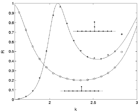
FIG. 2.: Reflection coefficient $\cal R$ as a function of $k$ (with $k$ between $\pi/2$ and $\pi$) when a chain with length $1$ (i.e., a single link) and $2$ are attached. Empty circles ($L=1$) and stars ($L=2$) correspond to the numerical solution of Eq.(11): in this figure, as well in the followings, as initial condition we choose a Gaussian with initial width $\gamma_{0}=40$ and momentum $k$. Solid lines correspond to the analytical prediction (27).

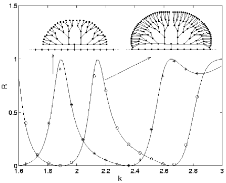
FIG. 3.: Reflection coefficient $\cal R$ as a function of $k$ when a Cayley tree with length $5$ and $6$ are attached. Empty circles ($L=6$) and stars ($L=5$) correspond to the numerical solution of Eq.(11). Solid lines correspond to the analytical prediction (see text). As required from the general argument in Section III, the values of $k$ for which one has perfect reflection (${\cal R}(k)=1$) for $L=5$ correspond to perfect transmission (${\cal R}(k)=0$) for $L=6$.

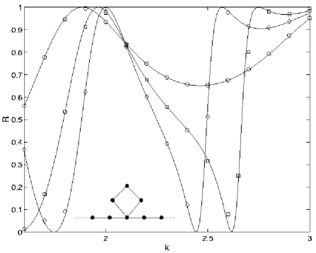
FIG. 4.: Reflection coefficient $\cal R$ as a function of $k$ when loops with $L=4$, $7$ and $10$ are inserted at a site of the unbranched chain. Empty circles ($L=4$), squares ($L=7$) and diamonds ($L=10$) are obtained from the numerical solution of Eq.(11). Solid lines correspond to the analytical prediction (33). The small figure represents a loop with $L=3$ inserted in the unbranched chain.

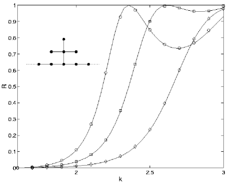
FIG. 5.: Reflection coefficient $\cal R$ as a function of $k$ when stars with $p=3$, $4$ and $6$ are inserted. Empty circles ($p=2$), squares ($p=3$) and diamonds ($p=5$) are obtained from the numerical solution of Eq.(11). Solid lines correspond to the analytical prediction (34). The inset represents the situation where the attached graph $G^{0}$ is a star with $p=3$.

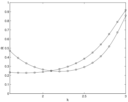
FIG. 6.: Reflection coefficient $\cal R$ as a function of $k$ when the complete graphs $K_{3}$ and $K_{11}$ are inserted at a site of an unbranched chain. Empty circles ($K_{3}$) and squares ($K_{11}$) are obtained from the numerical solution of Eq.(11). Solid lines correspond to the analytical prediction (35).

REFERENCES

- [1] S. Flach and C.R. Willis, Phys. Rep. 295, 181 (1998).
- [2] A. C. Scott, Nonlinear Science: Emergence and Dynamics of Coherent Structures, Oxford University Press (1999).
- [3] D. Hennig and G. P. Tsironis, Phys. Rep. 307, 333 (1999).
- [4] T. Nakayama, K. Yakubo, and R. L. Orbach, Rev. Mod. Phys. 66, 381 (1994).
- [5] M. Peyrard and A. R. Bishop, Phys. Rev. Lett. 62, 2755 (1989).
- [6] Proceedings of the Conference on Future Directions of Nonlinear Dynamics in Physical and Biological Systems, Denmark edited by P. L. Christiansen, J. C. Eilbeck, and R. D. Parmentier [Physica D 68, 1-186 (1993)].
- [7] Y. S. Kivshar and G. P. Agrawal, Optical Solitons: from Fibers to Photonic Crystals, San Diego, Academic Press (2003).
- [8] D. N. Christodoulides and E. D. Eugenieva, Phys. Rev. Lett. 87, 233901 (2001); Opt. Lett. 26, 1876 (2001).
- [9] P. G. Kevrekidis, D. J. Frantzeskakis, G. Theocharis, and I. G. Kevrekidis, Phys. Lett. A 317, 513 (2003).
- [10] A. R. McGurn, Phys. Rev. B 61, 13235 (2000); ibid. 65, 075406 (2002).
- [11] P. G. Kevrekidis, K. Ø. Rasmussen, and A. R. Bishop, Int. J. Mod. B 15, 2833 (2001).
- [12] M. J. Ablowitz, B. Prinari, and A. D. Trubatch, Discrete and Continuous Nonlinear Schrödinger Systems, University Press (2004).
- [13] H. S. Eisenberg, Y. Silberberg, R. Morandotti, A. R. Boyd, and J. S. Aitchison, Phys. Rev. Lett. 81, 3383 (1998).
- [14] R. Morandotti, U. Peschel, J. S. Aitchison, H. S. Eisenberg, and Y. Silberberg, Phys. Rev. Lett. 83, 2726 (1999).
- [15] A. Trombettoni and A. Smerzi, Phys. Rev. Lett. 86, 2353 (2001).
- [16] B. A. Malomed and M. I. Weinstein. Phys. Lett. A 220, 91 (1996).
- [17] D. B. Duncan, J. C. Eilbeck, H. Feddersen, and J. A. D. Wattis, Physica D 68, 1 (1993).
- [18] S. Flach and K. Kladko, Physica D 127 61 (1999).
- [19] J. Gomez-Gardenes, L. M. Floria, M. Peyrard, and A. R. Bishop, Chaos 14, 1130 (2004).
- [20] K. Forinash, M. Peyrard and B. A. Malomed, Phys. Rev. E 49, 3400 (1994).
- [21] V. V. Konotop, D. Cai, M. Salerno, A. R. Bishop and N. Grønbech-Jensen, Phys. Rev. E 53, 6476 (1996).
- [22] W. Krolikowski, and Yu. S. Kivshar, J. Opt. Soc. Am. B 13, 876 (1996).
- [23] A. B. Aceves, C. De Angelis, T. Peschel, R. Muschall, F. Lederer, S. Trillo, and S. Wabnitz, Phys. Rev. E 53, 1172 (1996).
- [24] R. Morandotti, H. S. Eisenberg, D. Mandelik, Y. Silberberg, D. Modotto, M. Sorel, C. R. Stanley, J. S. Aitchison, Opt. Lett. 28, 834 (2003).
- [25] A. E. Miroshnichenko, S. Flach, and B. A. Malomed, Chaos 13, 874 (2003).
- [26] S. Flach, A. E. Miroshnichenko, V. Fleurov, and M. V. Fistul, Phys. Rev. Lett. 90, 084101 (2003).
- [27] A. E. Miroshnichenko, S. F. Mingaleev, S. Flach, and Y. S. Kivshar, Phys. Rev. E 71, 036626 (2005).
- [28] F. Harary, Graph Theory, Addison-Wesley, Reading (1969).
- [29] M. K. Oberthaler and T. Pfau, J. Phys.: Condens. Matter 15, R233 (2003).
- [30] R. Fazio and H. van der Zant, Phys. Rep. 355, 235 (2001).
- [31] A. Birner, R. B. Wehrspohn, U. M. Gösele, and K. Busch, Adv. Mater. 13, 377 (2001).
- [32] P. A. M. Dirac, Proc. Camb. Phil. Soc. 26, 376 (1930).
- [33] F. Cooper, H. Shepard, C. Lucheroni, and P. Sodano, Physica D 68, 344 (1993).
- [34] A. Trombettoni and A. Smerzi, J. Phys. B 34, 4711 (2001).
- [35] R. E. Graham, D. E. Knuth, and O. Patashnik, Concrete Mathematics: A Foundation for Computer Science, Addison-Wesley, 1989.
- [36] I. E. Papacharalampous, P. G. Kevrekidis, B. A. Malomed, and D. J. Frantzeskakis, Phys. Rev. E 68, 046604 (2003).
- [37] M. J. Ablowitz and J. F. Ladik, J. Math. Phys. 17, 1011 (1976).
- [38] J. C. Eilbeck, P. S. Lomdahl, and A. C. Scott, Physica D 16, 318 (1985).
- [39] X. D. Cao and B. A. Malomed, Phys. Lett. A 206, 177 (1995).
- [40] N. L. Biggs, Algebraic Graph Theory, Cambridge University Press (1974).
- [41] I. Brunelli, G. Giusiano, F. P. Mancini, P. Sodano, and A. Trombettoni, J. Phys. B 37, S275 (2004).
- [42] R. Burioni, D. Cassi, P. Sodano, A. Trombettoni, and A. Vezzani, cond-mat/0502280.