Exact nonparametric inference for detection of nonlinearity

Abstract

We propose an exact nonparametric inference scheme for the detection of nonlinearity. The essential fact utilized in our scheme is that, for a linear stochastic process with jointly symmetric innovations, its ordinary least square (OLS) linear prediction error is symmetric about zero. Based on this viewpoint, a class of linear signed rank statistics, e.g. the Wilcoxon signed rank statistic, can be derived with the known null distributions from the prediction error. Thus one of the advantages of our scheme is that, it can provide exact confidence levels for our null hypothesis tests. Furthermore, the exactness is applicable for finite samples. We demonstrate the test power of this statistic through several examples.

^{† ‡}, ^†, ^†, and ^‡

1 Introduction

Nonlinear statistics such as correlation dimension and Lyapunov exponent [1] have been widely adopted in many fields to identify the underlying dynamical systems. However, even for a linear stochastic process with simple autocorrelation, these statistics could have finite and predictable values [2], thus without careful treatment, one may mistake a linear stochastic process for a nonlinear deterministic system when simply examining whether these statistics are convergent. This observation requires us to examine the basic properties of the underlying system in order to apply nonlinear analysis methods with greater confidence. Based on this viewpoint, to discriminate (stationary) linear stochastic processes from nonlinear deterministic systems, various methods have been developed, for example, the idea to investigate the orientations of the tangents to the system trajectory within given regions [6], the proposal to test the continuity of the underlying systems [7], and the suggestion to measure the mutual information and redundancy within the framework of information theory [8], to name but a few (see [3] for an extensive study).

In general, these methods focus on exploring the difference of some characteristic behaviors or properties between linear stochastic and nonlinear (deterministic) systems. In addition, a confidence level is usually preferred in order to indicate the reliability of the results. In practical situations, if only a scalar time series from an unknown source is available, the conventional approach for inference of the underlying system with the confidence level, as proposed by Theiler et al. [4], is to first assign a null hypothesis to the underlying system, and then apply the bootstrap method to produce a set of constrained-realization surrogate data, which should have the same statistic distribution as the original time series under the null hypothesis. Hence based on the empirical distribution of the adopted statistic of the surrogates and the original time series, one then determines whether to reject the null or not. However, since the exact knowledge of the statistic distribution is often not available, one will resort to certain discriminating criterion to help make the decision more objectively and determine the corresponding confidence level (if to reject). The popular discriminating criteria appearing in the literature of nonlinear (chaotic) time series analysis usually include two classes: parametric and nonparametric.

The parametric criterion assumes that the statistic follows a Gaussian distribution, and the distribution parameters, i.e. the mean and the variance, are estimated from the finite samples. One can determine whether to reject the null by examining whether the statistic of the original time series follows the statistic distribution of the surrogates. The corresponding confidence level of inference can be calculated from the estimated statistic distribution (see our discussions later); The nonparametric criterion [9] examines the ranks of the statistic values of the original time series and its surrogates. Supposes that the statistic of the original time series is $s_{0}$ and the surrogate values are $\{s_{i}\}_{i=1}^{N}$ given $N$ surrogate realizations. Then if the statistic of both the original time series and the surrogates follows the same distribution, the probability is $1/(N+1)$ for $s_{0}$ to be the smallest or largest among all of the values $\{s_{0},s_{1}...s_{N}\}$. Thus if $N$ is large, when one finds that $s_{0}$ is smaller or larger than all of the values in $\{s_{i}\}_{i=1}^{N}$, it is likely that $s_{0}$ instead follows a different distribution from that of $\{s_{i}\}_{i=1}^{N}$. Hence the criterion rejects the null hypothesis whenever the original statistic $s_{0}$ is the smallest or largest among $\{s_{0},s_{1}...s_{N}\}$, the false rejection rate is considered as $1/(N+1)$ for one-sided tests and $2/(N+1)$ for two-sided ones.

Note that the above two simple criteria are often adopted thanks to the difficulty in calculating the exact distribution of the nonlinear statistic under test. Although these two criteria are heuristic, they are often questionable in practice. For example, for the first criterion, the normality assumption may not approximate the actual distribution well. For the second, suppose that $s_{0}$ and $\{s_{i}\}_{i=1}^{N}$ follow the same distribution and let the range of the surrogate statistic be $\mathbf{A}$, while the support of the null distribution be $\mathbf{B}$, and $\mathbf{C}=\mathbf{B}\backslash\mathbf{A}$ be the complement set of $\mathbf{A}$ given $\mathbf{B}$. Then according to the rule, one rejects the null hypothesis whenever the original statistic $s_{0}\in\mathbf{C}$, and the actual false rejection rate is the probability $\Pr(s_{0}\in\mathbf{C}|\{s_{i}\}_{i=1}^{N})$, which usually will not simply depend on the number of surrogate realizations.

In this communication we will propose a new statistic, namely the Wilcoxon signed rank statistic, for detection of the potential nonlinearity of a scalar time series in the framework of Theiler et al. [4]. This statistic could be derived from the linear prediction error of the time series and proves to be a Wilcoxon variate under weak conditions. As an advantage, it has a known null distribution, thus inference with exact confidence level becomes possible based on the knowledge of the statistic distribution. Furthermore, this statistic could be applied to a wider range of linear stochastic process, including the stationary Gaussian colored noise discussed in [4]. We will introduce the detail of the derivation of the Wilcoxon signed rank statistic in Section 2. For demonstration, we will apply this statistic to several examples in Section 3. Finally we will summarize the whole work in Section 4.

2 Methodology

Now let us begin the introduction of the new statistic. As the first step, we would like to specify the null hypothesis $H_{0}$ to be tested. Given a stationary time series $\{x_{i}\}$ with finite coherence time [5], our objective is to detect if there exists nonlinearity of the underlying system. To perform a hypothesis test, we instead assume that the time series $\{x_{i}\}$ is from a linear stochastic process with independent jointly symmetric innovations, which is the null hypothesis $H_{0}$ to be tested in our work. For the processes that are not consistent with $H_{0}$, they will be attributed to the alternative null hypothesis $H_{1}$. For clarity, let us explain with more detail (readers are also referred to the original works [4]). In general, the data generation processes can be classified into linear or nonlinear stochastic processes and linear or nonlinear deterministic systems. However, for linear deterministic systems such as a sine wave, since they usually appear very regular (their portraits in phase spaces are fixed points or limit cycles), it is not difficult to detect the underlying mechanism. Thus in this work we will exclude them from our discussions .

Also note that, theoretically it is possible that a linear stochastic process has asymmetric innovation terms. However, linear stochastic processes with symmetric innovations are often good approximations in many practical situations, e.g., the Gaussian distributions of the driving force of a Browning motion, the thermal noise in an electronic circuit, the channel noise in telecommunication etc. Thus within the scope of our discussion, when we reject the null hypothesis $H_{0}$, we will say that there is a high possibility that the time series is generated from a nonlinear system (either deterministic or stochastic) . And this result can be taken as the primitive step for further investigation of the underlying system, for example, model building.

For any stationary linear stochastic process, it can be presented by an autoregressive moving average (ARMA) process thanks to the Wold’s decomposition theorem. For convenience in the later discussion, whenever feasible, we will use a $p$-th order autoregressive ($AR(p)$) processes instead to describe a linear stochastic process with the concrete forms of

$$x_{i}=a_{0}+\sum\nolimits_{j=1}^{p}a_{j}x_{i-j}+\epsilon_{i}\text{,}$$ (1)

where $\epsilon_{i}$ denotes the innovation terms, which are assumed in our null hypothesis to be independent of $x_{i}$, mutually independent of each other and have a distribution with joint symmetry. By “joint symmetry” of a stochastic process $\{\epsilon_{i}\}$ we mean that there exists some constant $\mu$ so that $\{\epsilon_{i}-\mu\}$ and $\{\mu-\epsilon_{i}\}$ have the same joint distributions, i.e. the probability density function (PDF) $f(\epsilon_{1}-\mu,\epsilon_{2}-\mu,...)=f(\mu-\epsilon_{1},\mu-\epsilon_{2},...)$ [11]. Clearly, linear autocorrelated Gaussian processes examined in [4] are consistent with our null hypothesis. Yet the coverage could be extended to a wider range, e.g. the linear stationary processes with independent (not necessarily identical) and jointly symmetric innovations.

With the above null hypothesis, we then need to choose a discriminating statistic to determine whether to reject the null or not. To derive our statistic, let us first consider the problem of predicting $k$-step ahead value of a linear stochastic process $\{x_{i}\}$ with jointly symmetric innovations $\{\epsilon_{i}\}$. Let $\hat{x}_{i}^{k}$ be the prediction at time $i$ ($\hat{x}_{i}^{k}=x_{i+k}$ if $k\leqslant 0$), and $e_{i}^{k}=x_{i+k}-\hat{x}_{i}^{k}$ denote the corresponding prediction error. For the purpose of prediction, we choose the ordinary least square (OLS) linear predictor $\hat{x}_{i}^{k}=a_{i,0}+\sum\nolimits_{j=1}^{p^{\prime}}a_{i,j}\hat{x}_{i}^{k-j}$ with $a_{i,j}$ being the the $(j+1)$th coefficient of the OLS predictor, estimated based on the history $\{x_{i},x_{i-1},x_{i-2},...\}$. In general situations, the OLS predictor may not perform as well as other procedures like the forward/backward least-square algorithm, however, it does possess an interesting property that might not be shared by other algorithms. The fact is that, as proved in [11], when an OLS linear predictor is used to predict the $k$-step ahead value of a linear stochastic processes $\{x_{i}\}$ with jointly symmetric innovations, even if the fitting order of the predictor is misspecified (either lower or higher), and thus inaccurate estimated parameters are adopted for prediction, the distributions of the prediction error $e_{i}^{k}$ will still be symmetric about zero, i.e. $e_{i}^{k}$ and $-e_{i}^{k}$ share the same distribution. This fact immediately implies that the probability $\Pr(e_{i}^{k}>0)=\Pr(-e_{i}^{k}>0)=\Pr(e_{i}^{k}<0)=1/2$ when the distribution of $e_{i}^{k}$ is continuous so that the probability $\Pr(e_{i}^{k}=0)=0$ in the sense of Lebesgue measure (see [12] and [13, Lemma 10.1.24] for more details).

Let $\{I_{i}\}_{i=1}^{m}$ be an indicator series with $m$ data points so that $I_{i}(e_{i}^{k})=1$ if $e_{i}^{k}>0$ and $I_{i}(e_{i}^{k})=-1$ if $e_{i}^{k}<0$. Clearly $I_{i}$ is a Bernoulli variate uniformly distributed on $\{-1,1\}$, i.e. $\Pr(I_{i}=-1)=\Pr(I_{i}=1)=1/2$. With this knowledge, we can derive a class of linear signed rank statistics

$$SR_{m}=\sum\nolimits_{i=1}^{m}I_{i}(e_{i}^{k})\times S_{i}(rank(|e_{i}^{k}|))$$ (2)

to test our null hypothesis, where $\{S_{i}(\cdot)\}$ is the set of scores of the series $\{|e_{i}^{k}|\}_{i=1}^{m}$ with $rank(|e_{i}^{k}|)$ denoting the rank (in the ascending order) of the absolute value $|e_{i}^{k}|$ among $\{|e_{i}^{k}|\}_{i=1}^{m}$ [13, p. 252]. Here we choose $S_{i}(rank(|e_{i}^{k}|))=rank(|e_{i}^{k}|)$ so that

$$SR_{m}=\sum\nolimits_{i=1}^{m}i\times I_{i}(e_{i}^{k})$$ (3)

is the widely used Wilcoxon signed rank statistic, which is discretely distributed. One could obtain the full knowledge of the distribution by enumerating all of its possible values, however, this is an ineffective way especially when $m$ is large. A remedy to this problem is to use the Gaussian distribution $N(0,m(m+1)(2m\,+1)/6)$ for approximation based on the limit central theorem. In [14, chaper 2] it is shown that the approximation works well even for small numbers, say, $m=6$. Therefore in this work we will adopt the strategy of distribution approximation.

Since we know the distribution of the test statistic, based on the realization value of $SR_{m}$, we can determine whether to reject the null hypothesis with an exact confidence level. Take two-sided test as an example, if we want the type-I error (the false rejection rate of a correct null) to be less than $\alpha$, then we first find two critical values $n_{u}$ and $n_{l}$ such that $n_{u}$ is the largest integer satisfying $\Pr(SR_{m}>n_{u})<\alpha/2$ and $n_{l}$ is the smallest integer satisfying $\Pr(SR_{m}<n_{l})<\alpha/2$. If for a time series in test, its statistic $SR_{m}>n_{u}$ or $SR_{m}<n_{l}$, then we reject the null hypothesis. The false rejection rate is $\alpha$, or in other words, the confidence level to reject the null hypothesis is $1-\alpha$. The procedures to perform one-sided tests are similar, except that we need to locate only one critical value, $n_{u}$ or $n_{l}$, which instead satisfies $\Pr(SR_{m}>n_{u})<\alpha$ or $\Pr(SR_{m}<n_{l})<\alpha$ separately for right or left side test.

For a linear stochastic process consistent with our null hypothesis, in principle one would expect that the actual rejection rate will be the same as the nominal (pre-specified) one. However, for a nonlinear system violating the hypothesis, it would generally engender higher rejection rates because of the asymmetry of the prediction errors (especially for the surrogate data, see the discussion in the next section), which is the essential idea inside our method.

3 Numerical results

We will apply the above idea to test our null hypothesis for nonlinearity detection. The whole procedures go as follows: For each time series $\{x_{i}\}$ in test, we first predict its one-step ahead values $\{\hat{x}_{i}^{1}\}$ via the OLS linear predictor and calculate the prediction error . Suppose the error series $\{e_{i}^{1}\}_{i=1}^{m}$ has $m$ data points, then we use the normal distribution $N(0,m(m+1)(2m\,+1)/6)$ to find the critical values ($n_{u}$ and $n_{l})$ for two-sided test at the nominal confidence level of $95\%$. If the calculated Wilcoxon statistic $SR_{m}\notin$ $[n_{l}$, $n_{u}]$, then we can reject the null hypothesis with the false rejection rate of $5\%$. In the following we will demonstrate through several examples the power of our scheme for the null hypothesis test.

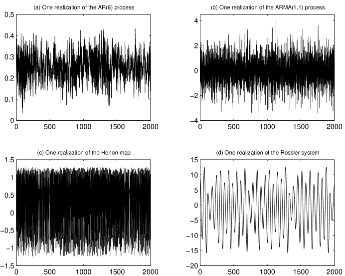
Figure 1: Waveform of a realization of: (a) the $AR(6)$ process, (b) the $ARMA(1,1)$ process, (c) the Henon map, and (d) the Rössler system.

The first example is an $AR(6)$ process $x_{i}=\sum\nolimits_{j=1}^{6}a_{j}x_{i-j}+\epsilon_{i}$ with coefficients $(a_{1},...,a_{6})=$ $(0.6$, $0$, $0.5$, $0$, $-0.6$, $0.3)$, where innovations $\{\epsilon_{i}\}$ are uniformly distributed on interval $[0$, $0.1]$ (symmetric about $0.05$). The second is an $ARMA(1,1)$ process, i.e. $x_{i}=a_{1}x_{i-1}+\epsilon_{i}-b_{1}\epsilon_{i-1}$ with parameters $a_{1}=b_{1}=0.5$, where innovation terms $\{\epsilon_{i}\}$ follow the normal distribution $N(0,1)$. The third data generation process (DGP) is the Hénon map [15] $H(x,y)=(y+1-\alpha x^{2},0.3x)$, where parameter $\alpha$ is uniformly drawn from the interval $[1.35$, $1.4]$. We will take out the first coordinate $x$ for test. The final case is the Rössler system [16] with continuous description equations of $(\dot{x},\dot{y},\dot{z})=(-y-z,x+0.15y,0.2+xz-cz)$, where parameter $c$ is uniformly drawn from the interval $[9.5$, $10]$. The sampling time is $0.1$ time units, and the observations for calculation are taken from the second coordinate $y$. The waveforms of the realizations of each DGP are plotted in Fig. 1.

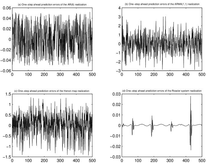
Figure 2: One-step ahead prediction errors ($p^{\prime}=6$) of a realization of: (a) the $AR(6)$ process, (b) the $ARMA(1,1)$ process, (c) the Henon map, and (d) the Rössler system.

Since usually one does not know the true order of an underlying process, a fitting order has to be specified for prediction. For this purpose, one may adopt the Akaike or Schwarz information criterion [22]. However, as aforementioned, if the underlying process of the test time series is linear stochastic with jointly symmetric innovations, misidentification of the fitting order would also lead to the symmetric prediction error. Thus we need not seek the optimal fitting order for our prediction. Instead, we could simply choose several fitting orders for all of the DGPs, say, those starting from $6$ to $10$. To indicate the power of our test scheme, for all of the DGPs in examination, we produce $1000$ realizations with $2000$ data points for each, and predict the one-step ahead values for the last $500$ data points. For demonstration, the prediction errors with $p^{\prime}=6$ are illustrated in Fig. 2 for each DGP (The results with other fitting orders are similar and thus not reported here). With the prediction errors, we calculate the Wilcoxon signed rank statistic to determine whether to reject the null or not. We record the rejection numbers of our null hypothesis and indicate them in Table 1. For the $AR(6)$ and $ARMA(1,1)$ processes, the rejection rates are nearly $5\%$, as we expect. For the Rössler system, although the rejection rates are various for different fitting orders, in general they are much higher than $5\%$, thus we can reject the null hypothesis. While for the Henon map, we see that the rejection rates are only slightly higher than the nominal one. The explanation may be that, in principle there is no universal scores in Eq. (2) that bring the most powerful signed rank statistic for all systems ([13, Theorem 10.1.19.]), and the sensitivity of this class of statistics might dramatically decrease for certain systems. The problem, however, could be relieved to some extent when we apply our framework to surrogate tests, as to be shown below.

In practical situations, one often has only a scalar time series on hand. Therefore, for the reliability of the test, we suggest that one first uses the bootstrap method, such as [4] and [17], to generate a number of surrogates, and then calculates the test statistic of the surrogates and determines whether to reject the null hypothesis or not. If the actual rejection rate is higher than the nominal one (i.e. the rate when the original time series is consistent with our null hypothesis), then we can safely reject the null hypothesis. For illustration, let us examine the previous examples again. For each example, we generate only one sample, and use the bootstrap method to generate $1000$ of its surrogates. In our test scheme, we adopt the temporal-shift algorithm in [17, 21] to generate surrogates since this algorithm does not require the Fourier transform and thus avoids some of its shortcomings . The main idea of the algorithm is that, if a time series $\{x_{i}\}$ is linear stochastic with the form of $x_{i}=a_{0}+\sum\nolimits_{j=1}^{p}a_{j}x_{i-j}+\epsilon_{i}$, then for any coefficients $\beta$ and $\gamma$, the surrogates $\{y_{i}^{\tau}=\beta x_{i}+\gamma x_{i+\tau}\}$ also follow linear stochastic forms with the constants of $(\beta+\gamma)a_{0}$ and the innovations of $\{\beta\epsilon_{i}+\gamma\epsilon_{i+\tau}\}$ respectively. A linear stochastic time series $\{x_{i}\}$ will always produce linear stochastic surrogates $\{y_{i}^{\tau}=\beta x_{i}+\gamma x_{i+\tau}\}$, therefore in principle we cannot reject the null hypothesis test via the Wilcoxon statistic. Following the suggestion in [21], in our calculations we let parameter $\beta$ be uniformly drawn from the interval $[0.6$, $0.8]$ and parameter $\gamma=(1-\beta^{2})^{1/2}$ to produce surrogates. The results of null hypothesis test are presented in Table 2, which appear different from those in Table 1. For the two linear stochastic processes, the rejection numbers decrease to zero. This is because that the original samples of the linear stochastic processes are not rejected in the tests (as $95\%$ of the samples are), therefore all its surrogates, which are essentially the addition of two segments of the original samples, will also not be rejected in the tests. However, the situation for nonlinear systems is different. Adding together two segments of the original samples from nonlinear systems increases the complexity, thus the rejection rates of the surrogates increase correspondingly compared to those in Table 1.

For comparison, we also generate $1000$ surrogates through the constrained-realization method [4], which preserves the linear correlation of the original time series but introduce some randomization to the phase of the Fourier transform. The computation results are indicated in Table 3, from which we could see that, the rejection rates of linear cases drop as well in contrast to those in Table 1. However, the rates of nonlinear cases remain close to those in Table 1, this is because, with the preservation of the linear correlation, the phase perturbation of the surrogates does not significantly affect the data structure, thus the rejection rates of the nonlinear systems are close to those in Table 1.

An further question is that: what will happen if the data in test is linear but with asymmetric innovation terms? To answer this question, let us see an example. We construct the following process

$$x_{i}=0.1+0.8x_{i-1}-0.5x_{i-2}+0.2x_{i-3}+\epsilon_{i}$$ (4)

with the innovation term $\epsilon_{i}$ following the $beta(2,5)$ distribution. Here

$$beta(\alpha,\beta)\equiv\frac{1}{B(\alpha,\beta)}s^{\alpha-1}(1-s)^{\beta-1}$$ (5)

with $B(\alpha,\beta)$ denoting the beta function. We choose the same computation settings as previously adopted. The results are summarized as follows,

1. For 1000 realizations generated by Eq. (4), the rejection numbers corresponding to the fitting orders ($6$ to $10$) are $98,99,103,105,109$ respectively.

2. For 1000 surrogates produced by the temporal shift algorithm based on one realization of Eq. (4), the rejection numbers corresponding to fitting orders are $0,0,0,0,0$ respectively.

3. For 1000 surrogates produced by the conventional constrained realization algorithm, the rejection numbers are $109,97,100,117,129$ respectively.

Based on the results, one can see that in $(3)$ one can correctly reject the null hypothesis but in $(2)$ one fails. Because the temporal shift algorithm is simply based on the linear superposition principle, although failing to reject the null hypothesis in $(2)$, it does tell us some useful information, i.e., the data in test is unlikely to be nonlinear (otherwise the rejection rate might obviously exceed the nominal, 5%, because of the superposition of the surrogates). In contrast, rejecting the null hypothesis in $(3)$ says that the data in test cannot be generated by a linear process with jointly symmetric innovation terms. Thus conbining the results in $(2)$ and $(3)$ might shed light on the underlying process, which is to be investigated in a future work.

As an application, we apply our scheme to examine an electrocardiogram (ECG) record during ventricular fibrillation (VF), a segment of which is plotted in Fig. 3 (for the details of data acquisition, see [19]). The segment in examination has $50,000$ data points, thus we use the temporal-shift method to generate $1000$ surrogates since it needs less computations than the constrained-realization algorithm. We also adopt the same fitting orders, from $6$ to $10$, to predict $100$ one-step ahead values. As the results, the correspondingly rejections of our null hypothesis are $566,$ $541,$ $530,$ $550,$ and $521$ (all out of $1000$ tests), a strong hint of nonlinearity.

4 Conclusion

To summarize, we have proposed an exact nonparametric inference scheme to detect the potential nonlinearity in a scalar time series. The exactness of our inference comes from the knowledge of the exact distribution of the adopted discriminating statistic, i.e., the Wilcoxon signed rank statistic, which indicates remarkable test power through the several examples examined in this communication. The advantages of this statistic include: it possesses the known null distribution. Thus it is easy for us to find the exact confidence interval for the inference of the underlying process. Furthermore, the exactness of the statistic distribution does not rely on the size of the sample time series in test. Comparatively, for many nonlinear discriminating statistics adopted in the literature, e.g. the correlation dimension, computations with too short samples may cause serious distortions.

XL was supported by a Hong Kong University Grants Council Competitive Earmarked Research Grant (CERG) number PolyU 5216/04E.

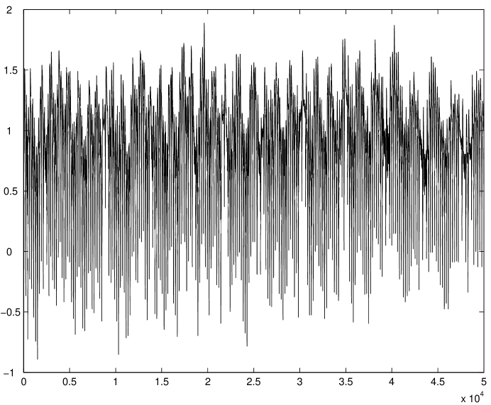
Figure 3: Waveform of a human electrocardiogram (ECG) record during ventricular fibrillation (VF)

Table 1: Numbers of rejections of the null hypothesis (out of 1000 replica) for data generation processes (DGPs) with different fitting orders.

DGP	Rejections for the fitting order of
	6	7	8	9	10
AR(6)	55	54	54	53	50
ARMA(1,1)	44	41	43	44	48
Henon	76	55	60	62	67
Rössler	990	442	752	298	458

Table 2: Rejections of the null hypothesis for $1000$ temporal-shift surrogates of DGPs with different fitting orders.

DGP	Rejections for the fitting order of
	6	7	8	9	10
AR(6)	0	0	0	0	0
ARMA(1,1)	0	0	0	0	0
Henon	432	307	308	203	207
Rössler	1000	553	1000	593	626

Table 3: Rejections of the null hypothesis for $1000$ constrained-realization surrogates of DGPs with different fitting orders.

DGP	Rejections for the fitting order of
	6	7	8	9	10
AR(6)	14	14	10	11	9
ARMA(1,1)	1	1	2	1	2
Henon	83	56	63	61	83
Rössler	992	449	753	301	460

References

- [1] H. Kantz, T. Schreiber, Nonlinear Time Series Analysis (Cambridge Univ. Press, Cambridge, 1997).
- [2] A. R. Osborne and A. Provenzale, Physica D 35, 357 (1989).
- [3] T. Schreiber and A. Schmitz, Phys. Rev. E 55, 5443 (1997).
- [4] J. Theiler, S. Eubank, A. Longtin, B. Gaidrikian and J. D. Farmer, Physica D 58, 77 (1992); J. Theiler and D. Prichard, Physica D 94, 221 (1996).
- [5] J. Theiler, P. S. Linsay, and D. M. Rubin, in Time Series Prediction: Forecasting the Future and Understanding the Past, ed. by A. S. Weigend and N. A. Gersbenfeld. Perseus Books, 1994, pp. 429-455.
- [6] D. T. Kaplan and L. Glass, Phys. Rev. Lett. 68, 427 (1992);
- [7] R. Wayland, D. Bromley, D. Pickett, and A. Passamante, Phys. Rev. Lett. 70, 580 (1993); D. T. Kaplan, Physica D 73, 38 (1994).
- [8] M. Paluš, V. Albrecht, and I. Dvořák, Phys. Lett. A 175, 203 (1993).
- [9] J. Theiler and D. Prichard, Fields Inst. Commun. 11, 99 (1997).
- [10] M. Pourahmadi, Foundations of Time Series Analysis and Prediction Theory (Wiley, New York, 2001).
- [11] J. M. Dufour, Econometrica 52, 209 (1984).
- [12] R. Luger, Journal of Econometrics 115, 259 (2003).
- [13] R. H. Randles and D. A. Wolfe, Introduction to the Theory of Nonparametric Statistics (Wiley, New York, 1979).
- [14] J. S. Maritz, Distribution-free Statistical Methods (Chapman &Hall, 1995).
- [15] M. Hénon, Comm. Math. Phys. 50, 69 (1976).
- [16] O. E. Roessler, Phys. Lett. A 57, 397 (1976).
- [17] T. Nakamura, X. Luo and M. Small, Phys. Rev. E 72, in press (2005).
- [18] A. Galka, Topics in Nonlinear Time Series Analysis with Implications for EEG Analysis (World Scientific, 2000).
- [19] M. Small, D. J. Yu, N. Grubb, J. Simonotto, K. Fox, and R. G. Harrison, Computers in Cardiology 27, 147 (2000).
- [20] M. Small, D. J. Yu, and R. G. Harrison, Phys. Rev. Lett. 87, 188101 (2001).
- [21] X. Luo, T. Nakamura, and M. Small, Phys. Rev. E 71, 026230 (2005).
- [22] K. P. Burnham, and D. R. Anderson, Model Selection and Multimodel Inference: A Practical-Theoretic Approach 2nd Edition (Springer, 2002).