Nonlocal competition and logistic growth: patterns, defects and fronts

Abstract

Logistic growth of diffusing reactants on spatial domains with long range competition is studied. The bifurcations cascade involved in the transition from the homogenous state to a spatially modulated stable solution is presented, and a distinction is made between a modulated phase, dominated by single or few wavenumbers, and the spiky phase, where localized colonies are separated by depleted region. The characteristic defects in the periodic structure are presented for each phase, together with the invasion dynamics in case of local initiation. It is shown that the basic length scale that controls the bifurcation is the width of the Fisher front, and that the total population grows as this width decreases. A mix of analytic results and extensive numerical simulations yields a comprehensive examination of the possible phases for logistic growth in the presence of nonlocal competition.

I Introduction

Recently, there is a growing interest in the spatial properties of logistic growth with nonlocal interactions Sakai ; Doebeli ; Bolker ; Tokita ; Hoopes ; Anderson ; Sayama ; Fuentes ; Birch ; shnerb ; Garcia . A variety of models have been introduced, including various types of interaction kernels, deterministic and stochastic evolution and growth or death rate that depends on the local population. A common feature found in all these models is the segregation transition, i.e., for small enough diffusion and for certain interaction kernels the homogenous state of the system becomes unstable and the steady state is spatially heterogenous. This feature turns out to be stable against the stochasticity induced by the discrete nature of the reactants, and the total carrying capacity (per unit volume) of the stochastic system depends on the details of the spatial segregation Birch ; Garcia .

In previous work shnerb , the general conditions for the integral kernel to allow for spatial segregation have been presented, and the existence of topological defects between ordered domains has been analyzed in detail for a logistic growth on a one dimensional array of patches with nearest-neighbor competition. Here, a comprehensive study of this reaction-diffusion equation is presented: short-range interactions are shown to yield spatial modulation of arbitrary large wavelength and different type of defects, the total population of the system admits nontrivial dependence upon the diffusion rate, and the dynamics of the system is studied, both for global initiation and for local initiation. The appearance of domains with different order parameter and the features of the boundaries between them is considered in detail for various situations.

Our starting point is the well-investigated Fisher-KPP equation fisher ; kol , first introduced by Fisher to describe the spread of a favored gene in population:

$$\frac{\partial c(x,t)}{\partial t}=D\nabla^{2}c(x,t)+ac(x,t)-bc^{2}(x,t).$$ (1)

Clearly, this equation is a straightforward generalization of the logistic growth to spatial domains, and allows for two steady states: an unstable state with $c(x)=0\ \forall x$ and the stable steady state $c(x)=a/b$. It was shown that, for any local initiation of the instability (i.e., $c(x)\neq 0$ on a compact domain) the invasion of the stable phase into the unstable region takes place via a front that moves in a constant velocity $v_{F}=2\sqrt{Da}$. The stability of this solution, the fact that the velocity is determined by the leading edge (”pulled front”) and the corrections to this expression due to stochastic noise associated with the discrete nature of the reactants derrida has been reviewed, recently, by various authors saarloos .

The FKPP equation is the simplest equation that describes the transition from unstable to stable steady state on spatial domains, and as such it fits many situations, from the spread of a disease by infection to the advance of a fire or new technology. Accordingly, this model has been widely studied from many points of view and has been generalized in many directions such as modified interaction terms, non linear diffusion and so on.

The process considered here, logistic growth with nonlocal competition, is described by the generalized FKPP equation:

$$\frac{\partial c(x,t)}{\partial t}=D\nabla^{2}c(x,t)+ac(x,t)-c(x,t)\int^{\infty}_{-\infty}\gamma(x,y)c(y,t)dy,$$ (2)

where $\gamma(x,y)$ is the interaction kernel, and the original FKPP process corresponds to the limit $\gamma(x,y)=\delta(x-y)$.

The motivation for the study of this process comes from one of the basic mechanisms in population growth, namely, the competition for common resource. In any autocatalytic system the multiplication of agents depends on various resources (energy, chemicals, water etc.). If there is only limited amount of the resource, its consumption leads to extinction, so generally any crucial resource should be deposited, and its availability dictates the saturation value for the population. As a concrete example let us look at vegetation merron ; lavee : the common resource needed for vegetation is water, and the rain corresponds to deposition of this resource. If the resource dynamics is much faster than that of the agents (shrubs, trees etc.), there is, at any time, a soil moisture profile that reflects the instantaneous vegetation configuration, and there is a depletion of this moisture at the spatial region around a biomass unit. Accordingly, the environmental conditions for a new agent at this region becomes hostile. Following arguments of this type one suggests that competition for common resource induces long range competition among agents via the depletion of the resource in the surroundings of an agent. Another examples may involve the competition for light huisman and cooperation among agents (symbiosis) that may yield ”negative competition” among the reactants.

Numerical simulations of the dynamics corresponds to Eq. (2) require space and time discretization. In this work the time evolution of the system is generated via forward Euler integration, where the time step is taken small enough such that further reduction of it do not effect the results. We simulate a system of discrete patches, where the hopping rate is proportional to the diffusion constant.

Let us present some a-priori considerations related to this system. There are few basic types of steady state solutions: first, it may happens that the steady state is homogenous: this may be the case if the long range competition is too small, or if the interaction kernel do not allow for the instability to occur shnerb ; Sayama . At some point in the parameter region a bifurcation may occur, and the homogenous states becomes unstable to modulation of wavelength $2\pi/k$. Right above the bifurcation one expects, though, to see an inhomogeneous (modulated) steady state. Far from the bifurcation point there are many unstable wavelengthes and some sort of mode competition takes place. In the other limit, i.e., very strong competition, one may expect that ”life” at a single patch forces all the other patches at finite range to be (almost) empty, so the steady state is sort of ”spiky” phase, where many active wavelengthes participate in the formation of localized bumps.

As we are looking at a dynamic system with no noise, few stable steady states may exist simultaneously, each admits its own basin of attraction in the space of possible initial conditions. Numerically, however, it turns out that only one important distinction should be made, namely, between local and global initiation: the initiation is ”local” if at $t=0$ there is finite support to the colony, while if the system begins with random small biomass that spreads all around it corresponds to global initiation. Within each of these subclasses, the numerics suggests that a generic initial condition will flow into a unique steady state.

This paper is organized as follows: in the second section the stable spatial configurations (steady states stable against small fluctuations) are presented: the conditions for an instability of the homogenous solution are reviewed and discussed, and the properties of the final state are identified in different parameter regions, leading to a characteristic ”phase diagram”. In the next section the appearance of defects (separating spatial regions with different order parameter phase) is studied. The fourth section deals with the ”spiky” phase, where many excited modes superimposed to yield a pattern of spikes and the typical defect is a combination of two depletion regions. In the fifth section there is a brief description of phases and defects in two spatial dimensions, and next the effect of the spatial segregation on the global population is considered. In the seventh section the dynamic properties of the model are discussed, including the velocity of the primary and the secondary Fisher fronts and the appearance of topological defect in the invaded region. Some comments and conclusions are presented at the end.

II Static properties

In this section we consider the steady state solutions for equation (2) on spatial domain of coupled, identical patches. The initiation is assumed to be global, i.e., the initial conditions are small, randomly spread, reactant population at each spatial patch. The model considered here allows for nontrivial spatial organization even in the absence of diffusion, due to the long range competition, and global initiation helps to see these features within reasonable simulation times. The differences, if any, between global and local initiation will be considered in the last section.

II.1 The bifurcation cascade

Let us consider the spatially discretized version of (2), i.e., an infinite one dimensional array of identical patches coupled to each other by diffusion and long range competition. The time evolution of the reactant density at the n-th site, $\widetilde{c}_{n}$, is given by:

$$\frac{\partial\widetilde{c}_{n}(t)}{\partial t} = \frac{\widetilde{D}}{l_{0}^{2}}[-2\widetilde{c}_{n}(t)+\widetilde{c}_{n+1}(t)+\widetilde{c}_{n-1}(t)]+a\widetilde{c}_{n}(t)$$ (3)

$$- b\widetilde{c}_{n}^{2}(t)-\widetilde{c}_{n}(t)\sum_{r=1}^{\infty}\widetilde{\gamma}_{r}[\widetilde{c}_{n+r}(t)+\widetilde{c}_{n-r}(t)].$$

where $\widetilde{D}$ is the diffusion constant and $a,b,\widetilde{\gamma}$ are the corresponding reaction coefficients. One may precede to define the dimensionless quantities,

$$\tau=at,\qquad c=b\widetilde{c}/a,\qquad\gamma_{r}=\widetilde{\gamma}_{r}/b,\qquad D=\frac{\widetilde{D}}{al_{0}^{2}}.$$ (4)

Note that the new ”diffusion constant” is $D=W^{2}/l_{0}^{2}$, where $W\equiv\sqrt{D/a}$ is the width of the Fisher front, so the dimensionless diffusion is determined by the ratio between the front width and the lattice constant. The continuum limit, though, is the limit where the front width is large in units of lattice spacing. With these definitions Eq. (3) takes its dimensionless form,

$$\frac{\partial c_{n}}{\partial\tau} = D[-2c_{n}+c_{n+1}+c_{n-1}]$$ (5)

$$+ c_{n}\left(1-c_{n}-\sum_{r=1}^{\infty}\gamma_{r}[c_{n+r}+c_{n-r}]\right),$$

that may be expressed in Fourier space [with $A_{k}\equiv\sum_{n}c_{n}e^{iknl_{0}}$] as,

$$\dot{A}_{k}=\alpha_{k}A_{k}-\sum_{q}\beta_{k-q}A_{q}A_{k-q},$$ (6)

where

$$\alpha_{k}\equiv 1-2D[1-cos(kl_{0})]$$ (7)

$$\beta_{k}\equiv 1+2\sum_{r=1}^{\infty}\gamma_{r}cos(rkl_{0}).$$ (8)

Following ns , one observes that $c_{n}$ is positive semi-definite so $A_{0}$ is always ”macroscopic”. Any mode is suppressed by $A_{0}$; accordingly, for small $\gamma_{r}$ one expects only the zero mode to survive. If, on the other hand, $\gamma_{r}$ increases above some threshold, bifurcation may occur with the activization of some other $k$ mode(s), and the homogenous solution becomes unstable. The condition for occurrence of such bifurcation is that:

$$g(k)=\beta_{k}+2\beta_{0}D[1-cos(kl_{0})]<0$$ (9)

fulfilled by some k. This is the situation where patterns appear and translational symmetry breaks. Right above the bifurcation there is only one active $k$ mode that dictates the modulation of the system. As $g(k)$ decreases further there are many active modes that compete with each other via the nonlinear terms of (6), and the linear stability analysis of the homogenous state may be irrelevant to the final spatial configuration.

II.2 Nearest neighbors interactions

In previous work, the properties of the system have been considered for the extreme case where the competition takes place only between neighboring sites ($\gamma_{r}=\gamma$ for $r=1$ AND $\gamma_{r}=0$ if $r>1$). For nearest neighbors (n.n) interaction of that type the only stable wave number is $k=\pi/l_{0}$, where $l_{0}$ is the lattice constant, and the bifurcation takes place at $\gamma<1/2$. The spatial state at this wave number is $u_{n}=A_{0}+A_{\pi}cos(n\pi/l_{0})$ and the spatial structure is of the form …ududud… (u=up, large amount of biomass, d=down, small amount). In the absence of diffusion spatial segregation takes the form 101010 , i.e., only the even (odd) sites are populated. Obviously, starting from generic random state different domains are crated with odd or even ”order parameter” and kinks (domain walls) emerge between different domains. As shown in shnerb , the structure of these topological defects, including their size (that diverges at the segregation transition) and their exact form may be calculated analytically.

II.3 Next nearest neighbors (n.n.n)

Quiet surprisingly, the increase of the competition radius by a single site takes us to a completely different regime. While in the case of nearest neighbors interaction the spatial modulation length and the competition length are the same, next nearest neighbors competition (and, accordingly, any interaction of longer range) may yield, upon tuning the parameters, spatial modulation of arbitrary large wavelength. This situation resembles the case of magnetic systems, e.g., an Ising chain: if the exchange interaction is only between nearest neighbors the equilibrium state admits only an up-down modulations, while n.n.n. interaction may yield large solitons, as shown by bak . In that sense the next n.n. case demonstrate the essential features of the long range competition model in a generic way, while at least part of the results may be inferred analytically.

The most general form of next nearest neighbors interactions is given by Eq. (5) with:

$$\gamma_{r}=\left\{\begin{array}[]{cc}\gamma_{1}&r=1\\ \gamma_{2}&r=2\\ 0&\texttt{else}\\ \end{array}\right.$$ (10)

The bifurcation threshold is defined now by the equation:

$$g(k)=1+2\gamma_{1}cos(kl_{0})+\gamma_{2}cos(2kl_{0})\beta_{k}+2\beta_{0}D[1-cos(kl_{0})]=0.$$ (11)

where $g$ has extremum points at $k_{1,2}=0,\pi$ and

$$k_{3}=arcos(\frac{-\gamma_{1}+\beta_{0}D}{4\gamma_{2}}).$$ (12)

If a real wavevector $k_{3}$ exists (i.e., at $|\frac{-\gamma_{1}+\beta_{0}D}{4\gamma_{2}}|<1$) it will be the minimum of $g(k)$ while $k_{1,2}$ are maxima. For the range of parameters where $k_{3}$ is imaginary the minima may be at $k=\pi$ and the modulation is of ”up-down” type, or $k=0$, where the homogenous state is stable. The resulting phase diagram, in the $\gamma_{1}-\gamma_{2}$ plane with zero diffusion, is presented in figure (1): In region I the homogenous state is stable, while in region II the bifurcation takes the system to the up-down mode, like the situation for n.n. interaction. In region III, however, $k_{3}$ dominate and modulations of any size may occur. The bifurcation line is given (in the presence of diffusion) by the two branches of the equation:

$$\gamma_{2}=\frac{1+2D-D^{2}+\gamma_{1}(5D-2D^{2})\pm\sqrt{1+4D+14D\gamma_{1}-2\gamma_{1}^{2}+12D\gamma_{1}^{2}}}{2D^{2}+4-16D}$$ (13)

that reduces, at the $D=0$ case, to the simple form:

$$\gamma_{2}=\frac{1\pm\sqrt{1-2\gamma_{1}^{2}}}{4}.$$ (14)

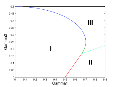
Figure 1: Phase diagram for next nearest neighbors competition at $D=0$. Region I is the homogenous, while II marks the up-down stable solution region similar to the n.n. case. In region III the wavevector $k_{3}$ (defined in the text) is stable and various wavenumbers may be active.

II.3.1 wavelength selection, mode competition and the spiky phase

From (12) it seems that the bifurcation wavelength is bounded from above by the interaction length. This, however, is not the actual situation on a discrete lattice: the wavelength inferred from Eq. (12), although bounded, is generically incommensurate with the lattice constant, and the system should choose a commensurate one. It turns out that, if the wavelength is rational (i.e., if $k_{3}=2\pi m/n$, where $m$ and $n$ admits no common denominator) the spatial modulation repeats itself after $n$ lattice sites. A typical example is the steady state obtained numerically for the case $m=7,n=20$ where a period-20 modulation appears, as demonstrated in Figure (2). At finite system the maximal $n$ allowed is of order of the system size, and only in an infinite system all rational fractions may be activated. Note that in an infinite system any change of the interaction parameters yields different wavelength, a phenomena that resembles the ”devil staircase” situation in spin systems bak .

Figure 2: Spatial structure of wavevector $k=14\pi/20l_{0}$. According to Eq. (12) one expects the modulation length to be $\lambda=20l_{0}/7$, but but discreteness of the lattice allows only for commensurate periodicity of 20 sites.

For finite system, though, there is a set of points along the bifurcation line that correspond to the allowed wavelengthes. Numerical simulation indicates that there is a basin of attraction around each of these points, i.e., if the interaction parameters $\gamma_{1}$ and $\gamma_{2}$ yields a prohibited wavelength the system flows into one of the closest allowed modulations. The overall structure is demonstrated in figure (3): close to an isolated point there is a basin of attraction, but further away from the bifurcation line these regions begin to overlap, and the system flows into some mixture of the closest allowed states, depending on its initial conditions. Deep in region III many wavenumbers are involved; the interaction parameters are relatively large, and instead of simple harmonic modulation the system flows, generically, into a spiky steady where the ”living colonies” are separated by the interaction length and are not effected by the competition between patches.

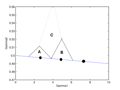
Figure 3: Basins of attraction for allowed states close to the bifurcation line (sketched). The straight line is an enlarged portion of the bifurcation line (I - III interface) of figure (1). The bold points on this line correspond to an allowed states, i.e., states with wavelength commensurate with the lattice size. Each possible wavevector admits a basin of attraction, like those denoted by A and B in the figure. Starting from $\gamma_{1}$,$\gamma_{2}$ values inside region A, for example, the system flows to the modulation corresponds to the bold point inside the triangle. Away from the bifurcation line (region C) few basins of attraction overlap and mode competition takes place. Even further away, deep in region III, the system is in the spiky phase: many active modes exist and their superposition yields the ”wave packet” characteristics of the spikes

Although the numerical examples presented here are for a system with next nearest neighbor competition and without diffusion, it is easy to extract from it the properties of the steady state in general. The effect of diffusion is to increase the size of the stable region so the bifurcation line of Figure (1) moves outward together with the pure and the spiky states. For interactions of longer range the parameter space is of higher dimensionality but all other features are essentially the same.

III Defects

The transition from the homogenous to the modulated state involves spontaneous breakdown of translational symmetry, and upon global initiation one may expect domain walls, or kinks, that separate spatial regions with different order parameter. The presence of these defect and their character is crucial for the understanding of the system response functions, e.g., its behavior under small noise: as there is no preference to one phase of the order parameter the kinks may move freely, while the ”bulk” of the domain is much more stiff. In the following paragraphs the characteristic defects for various phases are presented.

III.1 Domain walls

As mentioned above, the nearest neighbors competition leads, above the bifurcation threshold, to to appearance of an up-down modulation ($k=\pi$), and if there is no diffusion the steady state is the 0101010 configuration. Clearly there are two equivalent segregation of this type, namely, filled odd sites and empty even sites and vise versa. Accordingly, in case of global initiation (random ”seeds” are spread all around) one finds domains of the stable patterns with different parity, and domain walls (technically known as kinks or solitons) that separate these regions, as seen in figure (4). The nearest neighbor interaction is simple enough to allow for an analytic solution for the kink, and the numerical results confirm the predictions shnerb .

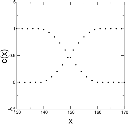
Figure 4: A typical kink of length $L=20$, an outcome of forward Euler integration of Eq. (5) (with n.n. competition) on 1024 lattice points with periodic boundary conditions and random initial conditions at $\gamma=0.505$ (just above the bifurcation).

In the presence of diffusion there is a ”smearing” of the above results: the homogenous state is stable for larger $\gamma$, and above the segregation threshold the steady state is ”smeared” from $...01010...$ to an ”up - down - up -down” form, and the kinks are not of finite size but admit exponentially decaying tails. See shnerb for details.

III.2 Phase shift

Unlike the nearest neighbor case, competition of longer range leads to instabilities with wavelength of more than one site, i.e., $c_{n}=A_{0}+A_{k}cos(nkl_{0})$ with general $k$. This opens the problem of defects between ordered regions. Inspired by the nearest neighbors example one may expect another types of kinks that separate different regions of ordered state. Surprisingly, this is not the case. Instead of getting kinks between different oriented regions of the activated wavenumber, one gets single oriented region with phase shift, namely, the spatial structure is of the form $c_{n}=A_{0}+Bcos(nkl_{0}+\phi)$, where $\phi$ is the phase shift between the actual solution and the predicted modulation $c_{n}=A_{0}+A_{k}cos(nkl_{0})$ and $B=A_{k}/cos\phi$.

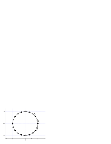
Figure 5: The set of different values of population size at different site is presented on the unit circle where the linear analysis predicts an instability with wavenumber $k=3\pi/5l_{0}$. The filled circles are the values of $cos(3n\pi/5l_{0})$, the solution predicted by the naive argument, and this is indeed a stable solution with finite basin of attraction [see Figure (7)]. It turns out, however, that generic initial conditions flow into a phase shifted solution where the population of the form $cos(3n\pi/5l_{0}+\phi)$ (shown in Figure (8). The value of $\phi$ is half of the angular distance between two close sites, here corresponds to the open triangles on the unit cycle.

On the unit cycle (Figure [5]) the meaning of this additional phase is a shift of all point by $\phi$. This shift may reduce the number distinct values in one cycle by one, as indicated in the example of Figure (5): here, instead of six distinct values taken by $c_{n}$ along one wavelength, there are only five. Both numerical simulations of the system dynamics, starting from random initial conditions, and stability analyzes of the possible steady state for arbitrary $\phi$ indicates that, although any $\phi$ corresponds to locally stable solution, the most stable $\phi$ equals to half of the angular distance between two adjusting points on the circle. In Figure (5) the actual phase shifted pattern is shown for $k=3\pi/5l_{0}$, while Figure (6) indicates that the most stable phase corresponds to $\phi/\phi_{0}=1/2$. As the Lyapunov exponent of any $\phi$ is negative, small perturbations around any $\phi$ value (in particular, $\phi=0$) decay. Figure (7) shows the corresponding stable mode with $\phi=0$ where the initial conditions are small perturbation around it. Figure (8), on the other hand, shows the final state with generic initial conditions, where the system flows to the most stable pattern with $\phi/\phi_{0}=1/2$.

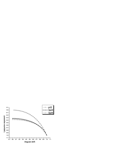
Figure 6: The Lyapunov exponent (in arbitrary units) for states of the form $cos(nk+\phi)$ is shown against $\phi$ (in units of $k/2$) for various wavenumbers. While the steady state is stable for any $\phi$, the most stable state corresponds to $k/2$, and

Figure 7: The steady state for the same parameters of figure (5), where the initial conditions are close to the $\phi=0$ solution, i.e., $c_{n}(t=0)=A_{0}+A_{k}cos(3\pi n/5)+\delta_{n}$, where $\delta_{n}$ is a small random number. The system flows into the $\phi=0$ case, in agreement with the local stability analysis presented in Figure (6).

Figure 8: Same as Figure (7), but now the initial conditions are generic $c_{n}(t=0)=\delta_{n}$. The system flows to the most stable steady state that corresponds, in this case, to $c_{n}=A_{0}+Bcos(3n\pi/5+\phi)$, with $\phi=3\pi/10$.

IV The spiky phase

Deep in region III of the phase diagram [Figure (1)] many wavevectors are excited, with strong mode competition between them, and the linear analysis picture based on Fourier decomposition becomes ineffective. Better insight into the system comes from a real space analysis: deep into region III the long range competition is strong, and within the effective interaction range new colony can not develop in the presence of a fully grown one. Accordingly, this phase is characterized by fully developed colonies separated by ”dead regions” of constant length that reflects the effective interaction length. In Fourier space, this corresponds to many active modes that build together a periodic structure of ”bumps”.

In case of global initiation, of course, defects may appear in the stable steady state as the system flows to different order parameter in different regions. Again, it is better to use the real space picture in order to describe these defects. The situation is close to what observed in the case of random sequential adsorption ads ; lavee : while an ”optimal” filling of the system admits a periodic structure of living patches with periodicity of, say, $L$ lattice points, it may happens that the distance between two fully developed sites is between L and 2L, and all the site in between should remain empty due to the long range competition. The emerging spatial configuration is of ordered regions (with coherence size that depends upon the dynamics) separated by ”domain walls”, where the width of these walls is taken from some distribution function between zero and the interaction effective length.

V Two dimensional system

Although all the analysis presented was in one dimension, the basic picture is the same for higher dimensionality. In particular, the bifurcation condition is similar, nearest neighbor interactions yields a ”checkerboard” phase above the bifurcation line, and the spiky phases is also observed.

For nearest neighbors interaction kinks between different regions (checkerboard parity) occurs. Because of the two dimensionality of the lattice the kinks might have any arbitrary spatial line, rather then straight line, as shown at figure (9). Those kinks are de-facto one dimensional topological defects, because of the periodic boundary conditions. On the other hand, the domain walls of Figure (10) seems to admit a real 2d features, although their topological character is not clear.

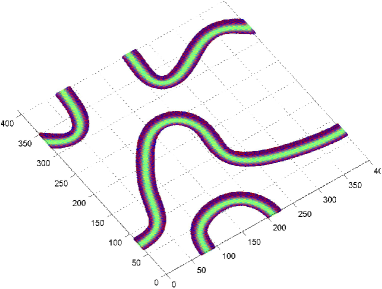
Figure 9: Spatial domains in two dimensional system, for logistic growth with nearest neighbors competition. The parameters are chosen to be above the bifurcation threshold, and the stable steady state is a ”checkerboard” with alternating filled and empty sites. Denoting a site by its coordinates $i,j$, there are two possible phases of the solution, correspond to filled $i+j\ \ odd$, empty $i+j\ \ even$ and vice versa. Here, the results of an Euler integration of the process for a $2d$ sample of $50x50$ sites with periodic boundary conditions is presented, where only the kinks separating regions of different order parameters are colored. The kinks here are non-contractible on the torus and correspond to one dimensional topological defects. The simulation parameters are $D=0,\ \gamma_{1}=0.2505$. Initial conditions are ”seed” population at each site taken randomly from a square distribution between $[0,0.01]$.

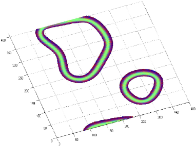
Figure 10: The same system and parameters as in Figure (9), for other choice of random initial conditions. Here the domain wall is contractible on the torus and the order parameter phases are different between the inside and the outside of the kink.

VI Global properties

VI.1 Upper critical diffusion

Let us turn back to the bifurcation condition, Eq. (9), in different representation:

$$\frac{\beta_{k}}{\beta_{0}}+2D[1-cos(kl_{0})]<0$$ (15)

where the $k$ considered is the one for which $\beta_{k}$ admits a global minimum. Clearly, this $k_{min}$ depends only on the form of the interaction kernel and is independent of its strength (if one multiplies all $\gamma_{r}$ by constant factor, the value of $k_{min}$ remains the same). Since the negative term in the instability condition $\frac{\beta_{k}}{\beta_{0}}$ cannot exceed $(-1)$, the absolute value of the right hand term should be even smaller to allow a periodic modulation of the stable steady state.

Assume, now, that the wavelength of the modulation is much larger than the lattice constant (as already required as one approaches the the continuum limit). In that case the approximation $2D[1-cos(kl_{0})]\approx Dk_{min}^{2}l_{0}^{2}$ holds, and since $D=(W_{F}/l_{0})^{2}$, this term is proportional to $(W_{F}/\lambda)^{2}$, where $\lambda$ is the period of the modulation. This implies that, independent of the strength of the long-range competition, bifurcation never takes place if the width of the Fisher front is larger than the period of the modulation. This statement holds up to a numerical factor (between zero and one) which determined by the form of the competition kernel.

Simple example that demonstrate these considerations is the case of nearest neighbors interaction. Here

$$g(k)=1+2\gamma cos(k)+2(1+2\gamma)D[1-cos(kl_{0})]$$ (16)

and the global minima is $k=\pi$. $g(k_{min})$ is

$$g(\pi)=1-2\gamma+4(1+2\gamma)D$$ (17)

so for any $\gamma$ there is an upper critical D

$$D_{c}=\frac{2\gamma-1}{4(1+2\gamma)}$$ (18)

above which no bifurcation takes place. This upper critical diffusion constant converges to a global value as $\gamma\to\infty$

$$D_{c}^{g}\equiv{D_{c},}_{\gamma->\infty}=\frac{1}{4}.$$ (19)

and no bifurcation takes place when the width of the Fisher front is of order of the modulation length. Intuitively this result may be understood as follows: suppose that the system is in its 010101 state, and suppose that the dynamics is discrete in time. If $D=1/4$ it implies that each filled site contribute $1/4$ to any of its neighbors, and then the system is frozen in its homogenous state with amplitude $1/2$ at each site. Generalizing this intuition to periodic modulation of arbitrary wavelength yields the same result, where the Fisher front width stands as a definition of an ”effective site”.

VI.2 Spatial segregation and total population

Given a system with long range competition, one may ask how the total population (integrated over all the spatial domain) or the average population density, depend on the phase of the system. Naively one expects the total population to grow with the diffusion constant, as faster spatial wandering helps an individual reactant to escape from the depleted region of an already existing colony. This, however, is not the case, as pointed out by Birch and Garcia : the size of the total population depends on the efficiency of segregation: strong segregation implies higher population (on average, since there are empty regions and living patches). Thus, decrease of diffusion implies higher total population density.

Clearly, the total population is given by the amplitude of the zero mode in Fourier decomposition of the population, (See Eq. 6). As long as the system is in its homogenous phase this quantity is diffusion independent and the total population depends only on the strength of the interaction, $A_{0}=1/\beta_{0}$. Right above the bifurcation, when only one excited mode ($k$) exists, the total population is proportional to $A_{0}=\alpha_{k}/(\beta_{0}+\beta_{k})$, and since $\alpha_{k}$ increases as $D$ decreases, so is the total population. In the case of one dimensional lattice with nearest neighbors interaction, for example, the dependence of the total occupancy of the sample on the diffusion constant may be calculated explicitly, since there is only one excited mode $k=\pi/l_{0}$. Here even far from the bifurcation point the amplitude of the zero mode is given by $A_{0}=\alpha_{k}/(\beta_{0}+\beta_{k})$. The total sum versus diffusion is, accordingly,

$$A_{0}=\left\{\begin{array}[]{cc}(1-4D)/2&D<D_{c}\\ 1/(1+2\gamma)&D>D_{c}.\end{array}\right.$$ (20)

Figure (11) shows the total sum versus diffusion for few situations. The numerical results indicate that the decay of average population is approximately linear. Note that, for the ”top hat” competition presented here, there seems to be a discontinuity at $D_{c}$ in two dimensions, while in $1d$ the total population is continuous at the transition.

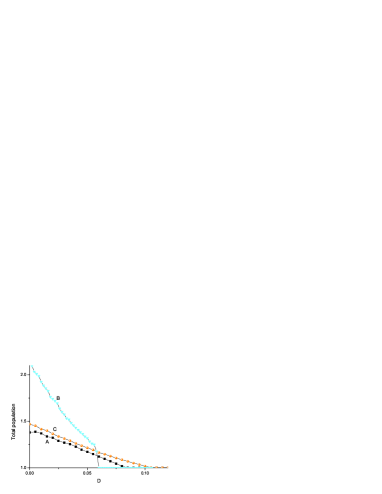
Figure 11: Total population versus diffusion coefficient for several situations. (A): $1d$ with nearest neighbors interaction (squares). (C): $1d$, n.n.n. interaction (circles). (B): $2d$, top hat interaction (triangles). The ”top hat” is constant interaction with all sites inside a circle of radius $3l_{0}$, and zero outside. In order to present all the results in the same panel, the population has been normalized, for each system, by its homogenous solution.

VII Local initiation: the dynamics of invasion and segregation

Along this paper, an analysis of the stable steady states of the logistic growth with long range competition was presented. As few stable steady solutions may exist simultaneity for the same set of parameters, the generic situation was identified numerically using global initiation, i.e., small random population at each site. In this section, the dynamics of growth is analyzed, where the initial conditions are a colony with compact support. For local logistic growth this problem was considered years ago by Fisher fisher and Kolomogorov kol . The invasion of the stable solution into the unstable one takes place via a front (the Fisher front) that propagates in constant velocity. This problem was considered by many authors in different contexts and was generalized to other cases of invasion into unstable state, see comprehensive review by van Saarloos saarloos .

As emphasized above, the system considered here may admit [in region II and III of figure (1)] two instabilities: the empty state is unstable against the homogenous one, while the homogenous solution breaks and yields a spatial modulation. Accordingly, if the system is initiated locally from a small colony of compact support one expects that two fronts propagate into the empty region: first the front associated with the homogenous state, and then the modulation (secondary instability) front hohenberg . These two fronts travel in different velocities. Generally, it is known that the Fisher velocity is determined by the leading edge (”pulled” fronts) and is related to the Lyapunov exponent that characterizes the relevant instability. Accordingly, the dynamics of our system is determined by two velocities: $v_{p}$, the velocity of the primary front (that interpolates between the empty and the homogenous state) and the modulation velocity $v_{s}$. While $v_{p}$ is $\gamma$ independent, the secondary front velocity $v_{s}$ depends on the characteristics of the long range competition. By tuning of $\gamma$, though, one may change the relative velocity between the primary and the secondary front. Both velocities may be calculated analytically using a saddle point method and taking into account the discreteness of the lattice points, as discussed in Appendix A. Generically, there are two possible scenarios for the takeover of an empty region by spatially modulated steady state: in the first case $v_{p}>v_{s}$ (see Figure 12) and the homogenous region between the primary and the secondary front grows linearly in time. This situation is very sensitive, as small perturbations (induced by the leading front) lead to spontaneous bifurcation of the homogenous region, a process that yields many structural defects (e.g., kinks) along the chain.

Figure 12: Snapshot of the one dimensional system, initiated locally from the left, where the primary velocity is higher then the secondary velocity. The two fronts are clearly shown, and the homogenous region between them is widening as time elapsed. The simulation assumes nearest neighbors competition with: D=0.04 and $\gamma=0.8$. Along time, defects (not shown) are generated at the tip of the secondary front due to the noise induced by the primary front.

In the second case the situation is different: if $v_{p}<v_{s}$ there is no homogenous region, and only one front exists. Its velocity is determined, of course, by the primary front velocity, but its shape is different (see Figure 13). In that case the sensitive homogenous region never exists, and the pattern formation process is robust, with no defects associated with the front kinetics.

Figure 13: Same as Figure 12, but now the velocity of the secondary front is higher than the velocity of the primary front. Since the secondary instability may appear only after the primary, the velocity of the whole front is determined by $v_{p}$. The parameters used are: D=0.04, $\gamma=2$.

VIII Conclusions and remarks

This paper attempt to present the various phases associated with the steady states of the logistic process on spatial domains with nonlocal competition. The main feature is, of course, the segregation transition that happens, as was shown, where the width of the Fisher front (associated with the homogenous solution) becomes shorter than the instability wavelength. Right above the bifurcation one finds a pattern dominated by a single wavelength, while far away from the bifurcation line the stable steady state becomes spiky. Each phase is associated with its own defects: phase shift close to the bifurcation, empty regions in the spiky phase, and domain walls (kinks) for the up-down phase of the nearest-neighbors interaction. It turns out that the segregation transition increase the overall carrying capacity per unit volume. In $1d$ the population is continues at the transition while in two dimensions discontinuity might occur.

Upon local initiation the system dynamics is governed by the relations between the velocities of the primary (empty to homogenous) and the secondary (homogenous to modulated) fronts. The numerics suggests that, while global initiation may yield ”disordered” structure with many defects per unit length, local initiation with the same parameters yields ordered structure unless the secondary front velocity is smaller that the primary one.

While in this work only rate equations of reaction-diffusion type has been considered, in recent numerical works of Birch and Young Birch and Garcia et. al. Garcia the stochastic motion of the individual reactants is taken into account. These stochastic models add two ingredients to the description presented here. First, the introduction of individual reactants (”Brownian bugs” young2 ) implies a threshold on the reactant concentration on single patch. Secund, there is a multiplicative noise associated with the stochastic motion of individual reactants. As shown in this work, many of the features associated with long range competition are independent of the discrete nature of individual reactants.

IX acknowledgements

The authors thank Prof. David Kessler for many helpful discussions. This work was supported by the Israeli Science Foundation, grant no. 281/03, and by Yeshaya Horowitz Fellowship.

X Appendix A

In this appendix the analytic expression for the secondary front velocity on a discrete lattice is obtained, via the saddle point argument (see levin ). For the sake of simplicity, only the case of nearest neighbors interaction is considered. In order to preform the same calculations for competition beyond the n.n. limit, one should first find numerically the steady state modulation and then follow the same procedure.

The evolution of a population is given by:

$$\frac{\partial c_{n}}{\partial t}=D[-2c_{n}+c_{n+1}+c_{n-1}]+c_{n}-c_{n}^{2}+c_{n}\gamma(c_{n+1}+c_{n-1}).$$ (21)

Denoting by $\delta_{n}$ the deviations from the homogenous solution, $c_{n}=A_{0}+\delta_{n}$, Eq. (21) is linearized to yield:

$$\frac{\partial\delta_{n}}{\partial t}=\alpha\delta_{n}+\beta(\delta_{n+1}+\delta_{n-1})$$ (22)

Where $\alpha=a-2bA_{0}+2A_{0}\gamma-2D/l_{0}^{2}$ and $\beta=D/l_{0}^{2}-A_{0}\gamma$. Assuming modulated solution of the form,

$$\delta_{n}=\left\{\begin{array}[]{cc}Ae^{ikl_{0}n+\Gamma(k)t}&\ \ n\ odd\\ Be^{ikl_{0}n+\Gamma(k)t}&\ \ n\ even\\ \end{array}\right.$$ (23)

and plugging (23) into (22) one gets

$$\Gamma(k)\left[\begin{array}[]{c}A\\ B\\ \end{array}\right]=\left[\begin{array}[]{cc}\alpha&\beta\cos(kl_{o})\\ \beta\cos(kl_{o})&\alpha\\ \end{array}\right]\left[\begin{array}[]{c}A\\ B\\ \end{array}\right].$$ (24)

The dispersion relations is given by:

$$\Gamma(k)=\alpha+\beta\cos(kl_{0}).$$ (25)

where the plus sign is chosen for the unstable modes. The solutions are of the form

$$\left[\begin{array}[]{c}c_{n}\\ c_{n+1}\\ \end{array}\right]=\left[\begin{array}[]{c}A\\ B\\ \end{array}\right]e^{ikx+\Gamma(k)t}.$$ (26)

If a solution represents a travelling front with velocity $v$ it is useful to define the coordinate system in the moving frame, $\zeta=x-vt$, to get

$$\left[\begin{array}[]{c}c_{n}\\ c_{n+1}\\ \end{array}\right]=\left[\begin{array}[]{c}A\\ B\\ \end{array}\right]e^{ik\zeta+ikvt+\Gamma(k)t}.$$ (27)

Using the saddle point method saarloos the two equations that determine the velocity are

$$f\equiv ivk+\alpha+2\beta cosh(kl_{0})=0$$ (28)

and

$$\frac{\partial f}{\partial k}=iv+2\beta_{0}sinh(kl_{0})=0.$$ (29)

In case of finite time steps one should replace $ivk$ by $(e^{-ikvdt}-1)/dt$ to get the appropriate corrections. Figure (14) shows the perfect fit between the solution of (28) and (29) and the numerical solution.

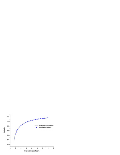
Figure 14: Comparison of the numerical simulation (triangles) and the theoretical prediction based on the saddle point method [Eqs. (28) and (29), solid line] for the velocity of the secondary front as a function of the interaction strength. The diffusion used is $D=0.04$ and the lattice constant is $l_{0}=1$, $dt=0.01$

XI Acknowledgements

We thank Prof. David Kessler for many helpful discussions and comments. This work was supported by the Israel Science Foundation (grant no. 281/03) and by the Yeshaya Horowitz Fellowship.

References

- (1) H. Sayama, M.A.M. de Aguiar, Y. Bar-Yam and M. Baranger, Phys. Rev. E 65, 051919 (2002).
- (2) M. A. Fuentes, M. N. Kuperman and V.M. Kenkre, Phys. Rev. Lett. 91, 158104 (2003).
- (3) N.M.Shnerb, Phys. Rev. E 69, 061917 (2004).
- (4) E. H. Garcia and C. Lopez. , Phys. Rev. E 70, 016216 (2004).
- (5) A. Sakai, Jour. Theor. Biol. 186 , 415 (1997).
- (6) M. Doebeli and T. Killingback, Theo. Population Biology 64, 397 (2003).
- (7) B.M. Bolker, Theoretical Population Biology 64, 255 (2003).
- (8) K. Tokita and A. Yasutomi, Theoretical Population Biology 63, 131 (2003).
- (9) K. Anderson and C. Neuhauser, Ecological modeling 155, 19 (2002).
- (10) F. Hoops at el., Jour. Theor. Biol. 210, 201 (2001).
- (11) D. Birch , W.R. Young, Private communication.
- (12) R. A. Fisher, Ann. Eugenics 7, 353, (1937).
- (13) A. Kolomogoroff, I. Petrovsky and N. Piscounoff, Moscow Univ. Bull. Math. 1,1 (1937).
- (14) E. Brunet, B. Derrida, J. Stat. Phys. 103, 269-282 (2001).
- (15) See, e.g., W. van Saarloos, Physics Reports 386, 29,(2003).
- (16) J.B. Wilson and A.D.Q. Agnew, Adv. Ecol. Res. 23, 263 (1992); R. Lefever and O. Lejeune, Bull. Math. Biol. 59, 263 (1997); J. von Hardenberg, E. Meron, M. Shachak and Y. Zarmi, Phys. Rev. Lett. 87 198101 (2001).
- (17) N.M. Shnerb, P. Sarah, H Lavee and S. Solomon, Phys. Rev. Lett. 90, 038101 (2003).
- (18) F.J. Weissing and J. Huisman, Jour. Theo. Biol. 168, 323 (1994).
- (19) P. Bak and R. Bruinsma, Phys. Rev. Lett. 49, 249 (1982).
- (20) D.R. Nelson and N.M. Shnerb, Phys. Rev. E 58, 1383 (1998), Appendix B.
- (21) See, e.g., J. Talbot, G. Tarjus, P. R.Van-Tassel, and P.Viot, Colloids Surf. A 165, 287 (2000), and references therein.
- (22) E. H. Garcia, C. Lopez. , Physica. D 199, 223-234 (2004).
- (23) See, e.g., M.C. Cross and P. Hohenberg, Rev. Mod. Phys. 65, 3, 851 (1993) and references therin.
- (24) W.R. Young , A.J. Roberts and G. Stuhne , Nature 412 328 (2001).
- (25) L. Pechenik, H Levine. cond-mat/9811020, (1998).