Dynamics of Small Perturbations of Orbits on a Torus in a Quasiperiodically Forced 2D Dissipative Map

Abstract

We consider the dynamics of small perturbations of stable two-frequency quasiperiodic orbits on an attracting torus in the quasiperiodically forced Hénon map. Such dynamics consists in an exponential decay of the radial component and in a complex behaviour of the angle component. This behaviour may be two- or three-frequency quasiperiodicity, or it may be irregular. In the latter case a graphic image of the dynamics of the perturbation angle is a fractal object, namely a strange nonchaotic attractor, which appears in auxiliary map for the angle component. Therefore, we claim that stable trajectories may approach the attracting torus either in a regular or in an irregular way. We show that the transition from quasiperiodic dynamics to chaos in the model system is preceded by the appearance of an irregular behaviour in the approach of the perturbed quasiperiodic trajectories to the smooth attracting torus. We also demonstrate a link between the evolution operator of the perturbation angle and a quasiperiodically forced circle mapping of a special form and with a Harper equation with quasiperiodic potential.

I Introduction

From the beginning of 1980s, much attention has been paid to studies of quasiperiodically forced systems. Indeed, systems with controllable ratios of incommensurate frequencies represent convenient models for the analysis of bifurcations of quasiperiodic regimes and of the mechanisms of transition from quasiperiodicity to chaos. Attention to this class of systems emerged also due to strange nonchaotic attractors (SNAs), which can generically occur there. A large number of works was devoted to the investigation of mechanisms of regular bifurcations [12, 13, 14, 15, 16, 17, 18, 19], irregular dynamical transitions [15, 16, 17, 18, 19, 20, 21, 22, 23, 24, 25] and attractor crises [26, 27, 28, 29, 30, 31, 32, 33] in quasiperiodically forced systems of different nature.

In most cases, interest in the dynamical systems is focused on the analysis of stationary dynamical regimes and their transformations. Researchers deliberately leave aside the dynamics of transient processes. In our humble opinion, such an approach is not wholly justified, since transient trajectories may visit wide regions of the phase space before drawing near the attractor. As a consequence, transient processes may contain extra information about the structure of invariant sets in the phase space of any dynamical system. Moreover, a change of the character of the transient process under variation of the controlling parameters of the system may precede transformations of the stationary dynamical regimes. In particular, a change of the character of the transient process may signal possible bifurcations and crises of attractors under further variation of the parameters of the system.

Here, we proceed with the investigation of the bifurcations and dynamical transitions in quasiperiodically forced systems, although we focus on dynamics of transient processes and their transformations. Our main goal is to show that a regular attractor may have an irregular transient process in its vicinity, and a complication of the transient may signal imminent destruction of the regular attractor under variation of the parameters of the system.

In the present work we consider the dynamics of small perturbations of stable quasiperiodic orbits with two incommensurate frequencies on an attracting torus. As a model system, we consider the quasiperiodically forced Hénon map, which can be interpreted as a Poincaré map of a hypothetical nonlinear oscillator driven by external biharmonic signal with irrational frequency ratio. A smooth closed invariant curve in the 3D phase space of the model map corresponds to a Poincare section of a 2D torus in the 4D phase space of such an oscillator. Therefore, we shall refer to such a smooth closed invariant curve as a “torus”. Evolution of a small perturbation of a trajectory on a stable torus consists of exponentially decaying radial component of the perturbation (what corresponds to the approach of the perturbed trajectory to the attracting invariant curve) and complex behaviour of the angle component of the perturbation, which characterizes a rotation of the perturbation vector around the invariant curve. We show that the dynamics of the angle component of the perturbation may have the character of a two- or three-frequency quasiperiodicity, or it may be irregular. In the first two cases a graphic image of such dynamics represents a two- or three-frequency torus, while in the latter case this image corresponds to a strange nonchaotic attractor. Note, that the attractor of the model system remains a smooth torus, while irregular transient process appears in its vicinity.

We analyse the global structure of the parameter space of the model system in the region of complex dynamical transitions consisting in the destruction of the smooth torus accompanied by the birth of a strange nonchaotic attractor or a divergence of trajectories. We demonstrate that the appearance of an irregular (in terms of angle) character of approach of stable trajectories to the attracting torus plays the role of a “precursor” of such transitions. Namely, the birth of a SNA via torus gradual fractalization [20, 21], intermittency [23, 24] and collision with a saddle torus [22], as well as the appearance of trajectory divergence via the collision of an attracting torus with a fractal basin boundary [26, 27], is preceded by the appearance of irregular dynamics of the perturbation angle. Note that the attractor of the system remains smooth while perturbed trajectories in its vicinity already demonstrate “strange” behaviour. On the other hand, regular torus bifurcations such as torus-doubling are accompanied by regular behaviour of the perturbation angle both before and after the bifurcation. We also discuss aspects of a link between the perturbation angle dynamics and a special circle mapping and with the Harper equation with a quasiperiodic potential.

The paper is organized as follows. In Sec. II we briefly observe the types of attractors and dynamical transitions in the parameter space of the model system. In Sec. III we obtain the equation of the evolution of the perturbation angle in explicit form, and discuss its connection with the Harper equation (Sec. IV). In Sec. V we analyse numerically different kinds of the perturbation angle dynamics and demonstrate their relationship with the types of dynamical transitions in the parameter space of the model system.

II Bifurcations and dynamical transitions in the quasiperiodically forced Hénon map

Our model system has the form:

$$\begin{array}[]{lll}x_{n+1}=f(x_{n},y_{n},\theta_{n})\equiv a-x_{n}^{2}-b\,y_{n}+\varepsilon\cos{\theta_{n}},\\ y_{n+1}=g(x_{n},y_{n},\theta_{n})\equiv x_{n},\\ \theta_{n+1}=\theta_{n}+2\pi\omega\pmod{2\pi},\end{array}$$ (1)

where the quasiperiodic force frequency parameter is chosen equal to the inverse golden mean value: $\omega=(\sqrt{5}-1)/2$.

The examples of typical attractors of the map (1) are presented in Fig. 1. At $a=1.09$, $\varepsilon=0.2$ (here and hereafter we set $b=0.3$) the attractor is a smooth closed invariant curve (“torus” T, Fig. 1(a)). With an increase of the nonlinearity parameter $a$, the torus T may bifurcate into a “double torus” 2T, which consists of a pair of smooth closed curves mapping into each other under iteration of the map, as shown in Fig. 1(b) where $a=1.445$, $\varepsilon=0.095$. (If $\varepsilon$ is small enough, one can also observe a second torus-doubling bifurcation, which gives four smooth closed curves. Note, that the number of torus-doubling bifurcations on the route to chaos depends upon the quasiperiodic force amplitude $\varepsilon$; this number may increase and tend to infinity as $\varepsilon$ goes to zero [34]. The mechanism for the termination of torus-doubling cascades in invertible systems is discussed in Ref. [35].) On the other hand, a different kind of torus-doubling bifurcation (torus “length-doubling” bifurcation [29]) can occur for sufficiently large values of $\varepsilon$. This bifurcation produces a special type of torus, which is characterised by the existence of two wraps of a single invariant curve; we will refer it to as a “double-wrapped torus” ${\rm T}_{2}$ (see Fig. 1(c) where $a=0.728$, $\varepsilon=0.36$). Strange nonchaotic and chaotic attractors of the map (1) are presented in Fig. 1(d) ($a=0.94$, $\varepsilon=0.312$) and Fig. 1(e) ($a=1.6$, $\varepsilon=0.135$), respectively.

The phase diagram of the map (1) in the $a-\varepsilon$ parameter plane ($b=0.3$) is shown in Fig. 2(a). The regions of different types of dynamical behaviour are shown in different tones. Torus T (white), double torus 2T (light-grey), double-wrapped torus ${\rm T}_{2}$ (light-grey). Regions of chaotic dynamics are shown in black. On the border between quasiperiodicity and chaos regions of SNA (dark-grey) exist. In the patterned area the map (1) has no attractor, and the trajectories go to infinity.

In Fig. 2(b) an enlarged fragment of the phase diagram in the region of complex dynamical transitions is presented. Different lines passing along the border of the region of quasiperiodic dynamics correspond to different dynamical transitions occurring at the exit from this region. The dashed line F corresponds to the birth of a SNA via gradual fractalization of the smooth torus T [20]. The dotted line I corresponds to the intermittent mechanism of the birth of a SNA [23] via collision of torus T with a saddle chaotic invariant set [24]. The combined line M corresponds to the birth of a SNA via band-merging collision of a double torus 2T with a saddle parent torus [22]. A transition B from the region of quasiperiodicity to divergence of trajectories occurs when the torus T destroys and transforms into a chaotic transient via collision with a saddle chaotic set on the fractal basin boundary [26, 27]. Arrows give the direction of movement in the parameter space for each transition to be observed.

III Perturbation angle dynamics and a special circle mapping

Let us take a smooth attracting torus of the map (1), given by invariant curve of the form

$${\rm T}_{\{a,b\}}:\{(x,y,\theta)\in{\bf R}^{2}\times{\bf T}^{1}|x=X_{\{a,b\}}(\theta),y=Y_{\{a,b\}}(\theta),\theta\in[0,2\pi)\}.$$ (2)

The pair of continuous and smooth functions $\{X_{\{a,b\}}(\theta),Y_{\{a,b\}}(\theta)\}$ can be obtained by solving the system of nonlinear functional equations

$$\left\{\begin{array}[]{ll}X(\theta+2\pi\omega)=a-X^{2}(\theta)-b\,Y(\theta)+\varepsilon\cos{\theta},\\ Y(\theta+2\pi\omega)=X(\theta).\end{array}\right.$$ (3)

In what follows we can omit mention of the dependence of these functions upon the parameters $\{a,b\}$ and write simply $\{X(\theta),Y(\theta)\}$, although we should keep in mind the link of $\{X(\theta),Y(\theta)\}$ with the system (3).

Take a reference quasiperiodic trajectory $\{(x_{n},y_{n},\theta_{n})\}_{n=0,1,\ldots,\infty}\in{\rm T}$, and consider a perturbed trajectory close to it starting with the same initial phase: $\{(x_{n}+\delta x_{n},y_{n}+\delta y_{n},\theta_{n})\}_{n=0,1,\ldots,\infty}$. Evolution of a small perturbation $\delta{\bf r}_{n}=(\delta x_{n},\delta y_{n})(n=0,1,\ldots,\infty)$ of the trajectory on torus in linear approximation is given by the following map

$$\begin{array}[]{ll}\left[\begin{array}[]{cc}\delta x_{n+1}\\ \delta y_{n+1}\end{array}\right]=\hat{\bf J}(x_{n},y_{n},\theta_{n})\left[\begin{array}[]{cc}\delta x_{n}\\ \delta y_{n}\end{array}\right],\\ \theta_{n+1}=\theta_{n}+2\pi\omega\pmod{2\pi},\end{array}$$ (4)

where

$$\hat{\bf J}(x,y,\theta)=\left[\begin{array}[]{cc}\frac{\partial f(x,y,\theta)}{\partial x}&\frac{\partial f(x,y,\theta)}{\partial y}\\ \frac{\partial g(x,y,\theta)}{\partial x}&\frac{\partial g(x,y,\theta)}{\partial y}\end{array}\right].$$ (5)

Coordinates $x_{n}$ and $y_{n}$ in the map (4) are taken at the corresponding points of the trajectory on the torus T: $x_{n}=X(\theta_{n})$, $y_{n}=Y(\theta_{n})$. For convenience, let us introduce terms

$$\begin{array}[]{ll}F_{x}(\theta_{n})=\left.\frac{\partial f(x_{n},y_{n},\theta_{n})}{\partial x_{n}}\right|_{x_{n}=X(\theta_{n}),\;y_{n}=Y(\theta_{n})},&F_{y}(\theta_{n})=\left.\frac{\partial f(x_{n},y_{n},\theta_{n})}{\partial y_{n}}\right|_{x_{n}=X(\theta_{n}),\;y_{n}=Y(\theta_{n})},\\ G_{x}(\theta_{n})=\left.\frac{\partial g(x_{n},y_{n},\theta_{n})}{\partial x_{n}}\right|_{x_{n}=X(\theta_{n}),\;y_{n}=Y(\theta_{n})},&G_{y}(\theta_{n})=\left.\frac{\partial f(x_{n},y_{n},\theta_{n})}{\partial y_{n}}\right|_{x_{n}=X(\theta_{n}),\;y_{n}=Y(\theta_{n})}.\end{array}$$

Now the map (4) can be rewritten as

$$\begin{array}[]{lll}\delta x_{n+1}=F_{x}(\theta_{n})\delta x_{n}+F_{y}(\theta_{n})\delta y_{n},\\ \delta y_{n+1}=G_{x}(\theta_{n})\delta x_{n}+G_{y}(\theta_{n})\delta y_{n},\\ \theta_{n+1}=\theta_{n}+2\pi\omega\pmod{2\pi}.\end{array}$$ (6)

In polar coordinates

$$\delta x=\delta r\cos{\varphi},\quad\delta y=\delta r\sin{\varphi}$$

the map (6) becomes

$$\begin{array}[]{lll}\delta r_{n+1}\cos{\varphi_{n+1}}=F_{x}(\theta_{n})\delta r_{n}\cos{\varphi_{n}}+F_{y}(\theta_{n})\delta r_{n}\sin{\varphi_{n}},\\ \delta r_{n+1}\sin{\varphi_{n+1}}=G_{x}(\theta_{n})\delta r_{n}\cos{\varphi_{n}}+G_{y}(\theta_{n})\delta r_{n}\sin{\varphi_{n}},\\ \theta_{n+1}=\theta_{n}+2\pi\omega\pmod{2\pi}.\end{array}$$ (7)

Substituting into (7) the values

$$\begin{array}[]{ll}F_{x}(\theta_{n})=-2X(\theta_{n}),&F_{y}(\theta_{n})=-b,\\ G_{x}(\theta_{n})=1,&G_{y}(\theta_{n})=0,\end{array}$$

we have

$$\begin{array}[]{lll}\delta r_{n+1}\cos{\varphi_{n+1}}=-\delta r_{n}[2X(\theta_{n})\cos{\varphi_{n}}+b\sin{\varphi_{n}}],\\ \delta r_{n+1}\sin{\varphi_{n+1}}=\delta r_{n}\cos{\varphi_{n}},\\ \theta_{n+1}=\theta_{n}+2\pi\omega\pmod{2\pi},\end{array}$$ (8)

and thus, eliminating the radius variable $\delta r$, we obtain

$$\begin{array}[]{ll}\cot{\varphi_{n+1}}=-[2X(\theta_{n})+b\tan{\varphi_{n}}],\\ \theta_{n+1}=\theta_{n}+2\pi\omega\pmod{2\pi}.\end{array}$$ (9)

In order to get an explicit map for the angle variable $\varphi$, one should take into account the conditions

$$\begin{array}[]{ll}\varphi_{n}\in[0,\pi/2)\cup[3\pi/2,2\pi)\Rightarrow\varphi_{n+1}\in[0,\pi),\\ \varphi_{n}\in[\pi/2,3\pi/2)\Rightarrow\varphi_{n+1}\in[\pi,2\pi),\end{array}$$ (10)

which immediately follow from the second equation of the system (8). Then, from (9) and (10) one can finally obtain the explicit mapping for the evolution of the perturbation angle variable $\varphi$:

$$\begin{array}[]{ll}\varphi_{n+1}=f(\varphi_{n},X(\theta_{n})),\\ \theta_{n+1}=\theta_{n}+2\pi\omega\pmod{2\pi},\end{array}$$ (11)

where

$$f(\varphi,X(\theta))=\left\{\begin{array}[]{ll}\arctan{[2X(\theta)+b\tan{\varphi}]}+(\pi/2),\quad\varphi\in[0,\pi/2)\cup[3\pi/2,2\pi),\\ \arctan{[2X(\theta)+b\tan{\varphi}]}+(3\pi/2),\;\varphi\in[\pi/2,3\pi/2).\end{array}\right.$$

Recall that $X(\theta)$ is a function of period $2\pi$. The map (11) represents a kind of a circle mapping under external quasiperiodic forcing. Note, that attractors of the map (11) must be symmetric with respect to a shift $\pi$ along the $\varphi$-axis. Therefore, the map (11) could be simplified to the form

$$\begin{array}[]{ll}\varphi_{n+1}=\arctan{[2X(\theta_{n})+b\tan{\varphi_{n}}]}+(\pi/2),\\ \theta_{n+1}=\theta_{n}+2\pi\omega\pmod{2\pi},\end{array}$$

by the choice of $\varphi\in[0,\pi)$.

Returning to the radial coordinate $\delta r$, one can see, that its dynamics is trivial. Indeed, for any small perturbation in a vicinity of the attracting torus T we immediately have:

$$\delta r_{n}=\sqrt{(\delta x_{n})^{2}+(\delta y_{n})^{2}}\sim\exp{(n\lambda_{1})}\sqrt{(\delta x_{0})^{2}+(\delta y_{0})^{2}}=\delta r_{0}\exp{(n\lambda_{1})},$$

where $\lambda_{1}<0$ is the largest nontrivial Lyapunov exponent, which characterizes stability of the torus T.

The analysis of the dynamics of the perturbation angle $\varphi$ on complex tori of the form $k\,{\rm T}\;(k=2,4,8,\ldots)$ in the map (1) requires trivial modification of the map (11). The last becomes cyclic:

$$\begin{array}[]{ll}\varphi_{n+1}=f(\varphi_{n},X^{(m)}(\theta_{n})),\\ \theta_{n+1}=\theta_{n}+2\pi\omega\pmod{2\pi},\end{array}$$

where $n=kp+m$, $p$ is integer, $m=1,2,\ldots,k$, and $\{X^{(m)}(\theta)\}$ is a set of functions determining a set of $k$ smooth closed curves which the complex torus $k\,{\rm T}$ consists of. On the other hand, for analysis of the dynamics of the perturbation angle $\varphi$ on the double-wrapped torus ${\rm T}_{2}$ it is convenient to redefine the phase variable $\theta$ on the interval $[0,4\pi)$ and to rewrite the map (11) in the following form:

$$\begin{array}[]{ll}\varphi_{n+1}=f(\varphi_{n},X_{(2)}(\theta_{n})),\\ \theta_{n+1}=\theta_{n}+2\pi\omega\pmod{4\pi},\end{array}$$

where $X_{(2)}(\theta)$ is a function of the period $4\pi$ defining the double-wrapped torus ${\rm T}_{2}$.

IV A link to the Harper equation

Let us make a change of the variable in the map (9): $\tilde{u}_{n}=\tan{\varphi_{n}}$. Then, one can write:

$$\begin{array}[]{ll}\tilde{u}_{n+1}=-[b\tilde{u}_{n}+2X(\theta_{n})]^{-1},\\ \theta_{n+1}=\theta_{n}+2\pi\omega\pmod{2\pi}.\end{array}$$ (12)

Then, introducing $u_{n}=b^{1/2}\tilde{u}_{n}$, one obtains:

$$\begin{array}[]{ll}u_{n+1}=-[u_{n}+2b^{-1/2}X(\theta_{n})]^{-1},\\ \theta_{n+1}=\theta_{n}+2\pi\omega\pmod{2\pi}.\end{array}$$ (13)

Since the function $X(\theta)$ is $2\pi$-periodic, it can be decomposed into Fourier series:

$$X(\theta)=a_{0}/2+\sum_{k=1}^{\infty}{A_{k}\cos{k(\theta+\phi_{k})}}.$$ (14)

Fourier coefficients $\{A_{k}\}_{k=1\ldots\infty}$ and $\{\phi_{k}\}_{k=1\ldots\infty}$ can be obtained from numerical solution of the functional equation (3). For the case of small values of the quasiperiodic force amplitude $\varepsilon$ (see the map (1)), one may take into account the first terms of the Fourier series only and obtain

$$\begin{array}[]{ll}u_{n+1}=-[u_{n}+b^{-1/2}a_{0}+2b^{-1/2}A_{1}\cos{(\theta_{n}+\phi_{1})}]^{-1},\\ \theta_{n+1}=\theta_{n}+2\pi\omega\pmod{2\pi}.\end{array}$$ (15)

Introducing parameters $E=-b^{-1/2}a_{0}$, $\lambda=b^{-1/2}A_{1}$, the map becomes

$$\begin{array}[]{ll}u_{n+1}=-[u_{n}-E+2\lambda\cos{(\theta_{n}+\phi_{1})}]^{-1},\\ \theta_{n+1}=\theta_{n}+2\pi\omega\pmod{2\pi},\end{array}$$ (16)

which reduces to the Harper equation with a quasiperiodic potential after a standard change of the variables $u_{n}=\psi_{n-1}/\psi_{n}$:

$$\psi_{n+1}+\psi_{n-1}+2\lambda\cos{(2\pi\omega n+\phi)}\psi_{n}=E\psi_{n},$$ (17)

where $\phi=\theta_{0}+\phi_{1}$ is a phase shift.

The states of the wave function in the Harper equation are known to be related to the dynamical regimes of the map (16). The extended states in the subcritical region ($\lambda<1$) correspond to tree-frequency tori, while the localized states in the supercritical region ($\lambda>1$) are associated with SNAs in the map (16). A two-frequency torus of the map (16) corresponds to the non-normalizable wave function and to the gap in the energy spectrum.

In Fig. 3 the standard phase diagram of the Harper map (16) is presented. The extended phase (Ext.) is shown in white, and the localized phase (Loc.) is denoted by gray. The Gap regions are shown in the light-gray tone. In order to obtain this diagram, we used the following technique. Each dynamical regime of the map (16) was characterized by the non-trivial Lyapunov exponent $\sigma$ and the phase sensitivity exponent $\delta$ [11]. These exponents take values $\sigma=0$ and $\delta=0$ for a three-frequency torus, $\sigma<0$ and $\delta=0$ for a two-frequency torus, and $\sigma<0$ with $\delta>0$ for the case of a SNA.

The link from the Harper equation to the map (11) suggests that the configuration of the phases on the diagram (Fig. 3) can be related to the structure of sets in the parameter space of the quasiperiodically forced Hénon map. Indeed, in the next section we will show that regions of different perturbation angle dynamics are organized as “tongues” of two- and three-frequency quasiperiodicity or of a complex behaviour corresponding to a SNA.

V Angular dynamics of perturbations in the context of torus bifurcations

Now we will focus on the angle dynamics of small perturbations in a vicinity of the torus T. Suppose we have a trajectory starting from the initial phase $\theta_{0}$ on the torus and examine its small perturbation with an arbitrarily chosen initial angle $\varphi_{0}$. Further evolution of the perturbation angle $\varphi$ is determined by the map (11). In what follows, we choose a few sets of the parameters $(a,\varepsilon)$ such that a smooth torus T exists in the map (1) and consider a dynamics of the map (11) at the same parameter values.

At $a=0.8$, $\varepsilon=0.1$ the attractor of the map (11) represents a smooth torus $\varphi=\Phi(\theta)$ shown in Fig. 4(a). Note that tori of the map (11) may have different topology, demonstrate one or many wraps on the circle $\varphi\in[0,2\pi)$ and consist of one or two segments, as shown in the Fig. 4(b) where $a=1.3$, $\varepsilon=0.5$. The 2D map (11) is characterized by two Lyapunov exponents. A trivial Lyapunov exponent associated with the quasiperiodic variable $\theta$ is equal to zero, while a nontrivial Lyapunov exponent in our cases takes the value $\sigma=-0.1170$ for the first set of parameter values and $\sigma=-0.9755$ for the second set. The angle variable $\varphi_{n}$ of an arbitrarily chosen perturbation on the torus T asymptotically behaves as $(\varphi_{n}-\Phi(\theta_{n}))\sim\exp(\sigma n)$, tending to $\Phi(\theta_{n})$ as $n\rightarrow\infty$. Thus, asymptotic dynamics of the perturbation angle $\varphi_{n}$ in our cases represents a regular two-frequency quasiperiodic motion.

As the parameters of the maps are varied to $a=0.85$, $\varepsilon=0.077$, the two-frequency torus of the map (11) disappears via the backward saddle-node bifurcation, and a three-frequency torus appears. A trajectory generated by the map (11) then uniformly fills a 2D torus $\{\varphi\in[0,2\pi),\theta\in[0,2\pi)\}$ (see Fig.4(c)). Strictly speaking, in this situation the map (11) does not possess an attractor, since it is characterized by two zero Lyapunov exponents. Thus, the dynamics of the perturbation angle $\varphi_{n}$ is regular and represents a three-frequency quasiperiodic motion.

On the other hand, as the parameters change to $a=0.9$, $\varepsilon=0.28$, the two-frequency torus of the map (11) destroys via phase-dependent mechanism with the birth of a strange nonchaotic attractor shown in Fig. 4(d). Note that the nontrivial Lyapunov exponent remains negative ($\sigma=-0.7747$). The angle variable $\varphi_{n}$ of an arbitrarily chosen perturbation in a vicinity of the torus T asymptotically behaves as $(\varphi_{n}-\Phi(\theta_{n}))\sim\exp(\sigma n)$ as $n\rightarrow\infty$, where $\Phi(\theta)$ is a fractal-like function characterized by non-differentiability and upper/lower semicontinuity [4]. As a result, the dynamics of the perturbation angle $\varphi_{n}$ is irregular. A graphic image of such dynamics is a trajectory on a strange nonchaotic attractor of the map (11).

In order to observe a configuration of regions corresponding to different types of dynamics of the perturbation angle variable $\varphi$ in the $a-\varepsilon$ parameter plane we need to combine the results obtained for the attractors of the maps (1) and (11). Such a combined phase diagram is presented in Fig. 5(a). The regions of chaos, SNA and chaotic transient in the map (1) are shown in black, dark-grey and pattern, respectively (the same as in Fig. 2(a)). The regions of the existence of a smooth attractor (i.e. T, 2T and ${\rm T}_{2}$ ) of the map (1) are subdivided according to the following principle: the white tone (1,4) denotes regions of three-frequency quasiperiodic dynamics of the angle variable $\varphi$ (three-frequency torus in the map (11)), the light-grey tone (2,5,7) shows regions of two-frequency quasiperiodicity of the perturbation angle $\varphi$ (two-frequency torus in the map (11)), and the grey tone (3,6,8) corresponds to regions of irregular dynamics of the angle $\varphi$ (SNA in the map (11)). An enlarged fragment of the diagram in the region of complex dynamical transitions in the model map (1) is shown in Fig. 5(b).

From Fig. 5(a) one can see that the configuration of regions of different behaviour of $\varphi$ is rather specific. The regions of a two- or three-frequency quasiperiodicity and of a SNA are organized as Arnold tongues. Recall that analogous tongues of the localized and extended phases were observed for the Harper equation (Fig. 3). However, the shapes of the tongues in Fig. 5(a) are distorted compared with those in Fig. 3. This distortion is associated with the non-rigorous transition from the Eq. (13) to Eq. (15), where only first terms of the Fourier series (14) were taken into account.

The line D (${\rm T}\rightarrow 2{\rm T}$) on the phase diagrams (Fig. 5(a),(b)) correspond to the usual torus-doubling bifurcation in the map (1). The line L (${\rm T}\rightarrow{\rm T}_{2}$) denotes the torus length-doubling bifurcation, which leads to the birth of a double-wrapped torus ${\rm T}_{2}$. The lines F, I, M and B in Fig. 5(b) denote the same dynamical transitions on the exit from the quasiperiodicity region that in Fig. 2(b).

Proceeding from Figs. 5(a),(b), let us analyze the dynamics of perturbations on the tori T and 2T at the threshold of the complex transitions F, I, M and B. On the phase diagrams one can see that all the regions of SNA, chaos and chaotic transient adjoin to the quasiperiodicity regions shown in the gray tone (and denoted by the numbers 3 and 6), corresponding to the existence of irregular dynamics of the perturbation angle variable $\varphi$. Thus, we can claim that the onset of irregular behavior of the perturbation angle $\varphi$ on the torus T precedes the following transitions: destruction of a smooth torus T and the birth of a SNA via fractalization (route F) and intermittency (route I) scenarios, destruction of a smooth torus T and the appearance of a chaotic transient via collision of the smooth torus T with a fractal basin boundary (route B). In the same way, the appearance of irregular behavior of the perturbation angle $\varphi$ on the double torus 2T precedes the destruction of the double torus 2T and the birth of a SNA via collision of 2T with the saddle parent torus (route M). It is important to note that all the transitions mentioned have phase-dependent mechanisms, as follows from their analysis in terms of rational approximations [21, 24, 27].

On the other hand, the lines of regular bifurcations such as torus doubling (D) and torus length-doubling (L) separate regions shown in light-gray tone corresponding to the existence of two-frequency quasiperiodic dynamics of the perturbation angle variable $\varphi$. Note, that regular tori bifurcations have phase-independent character (for instance see Ref. [13]). Thus, numerical analysis shows that phase-independent bifurcations of tori in the model map (1) are accompanied by regular behavior of small perturbations on a torus.

In our opinion, the connection between the behaviour of perturbations on a torus and the types of torus bifurcations is a problem of significant mathematical interest. Recently, two of us (Jalnine and Osbaldestin) suggested a partial solution of this problem for the case of torus-doubling bifurcation [35]. We introduced Lyapunov vectors as basis directions of contraction for an element of phase volume in a vicinity of the torus and shown that torus-doubling can occur only if the dependence of the Lyapunov vectors upon the angle coordinate $\theta$ on torus is smooth. We have also shown that the appearance of a non-smooth dependence of the Lyapunov vectors upon the angle coordinate on torus terminates the line of torus-doubling bifurcation on the parameter plane. Note that, after sufficiently large number of iterations, an arbitrarily chosen initial perturbation vector of the form $\delta{\bf r}_{0}=(\delta x_{0},\delta y_{0},0)$ on the torus T (see Sec. III) in a typical case tends to the leading Lyapunov vector, i.e., that corresponding to the largest Lyapunov exponent. Obviously, the regular dynamics of perturbations on the torus is associated with a smooth dependence of the Lyapunov vectors upon the angle coordinate $\theta$ on the torus, while the appearance of a SNA in the dynamics of the perturbation angle $\varphi$ manifests the onset of a non-differentiable dependence of the Lyapunov vector upon the coordinate $\theta$. The latter observation reveals the reason for regularity of the dynamics of $\varphi$, which accompanies regular torus bifurcations (e.g. doubling or length-doubling of a torus). However, the reason for irregularity in the behaviour of $\varphi$ on the threshold of phase-dependent transitions (such as torus fractalization, intermittency etc.) is still unrevealed and worthy of further study.

VI Conclusion

In the present work we investigated the dynamics of small perturbations of trajectories on an attracting torus in the quasiperiodically forced Hénon map. We have shown that dynamics of the angle variable of a perturbation may be a two- or three-frequency quasiperiodicity, or it may have irregular character. In the last case the graphic image of such dynamics is a trajectory on a strange nonchaotic attractor. It was also shown that the appearance of irregular character in the approach of trajectories to an attracting torus precedes the destruction of such a torus via phase-dependent mechanisms with the birth of a strange nonchaotic attractor or of a chaotic transient.

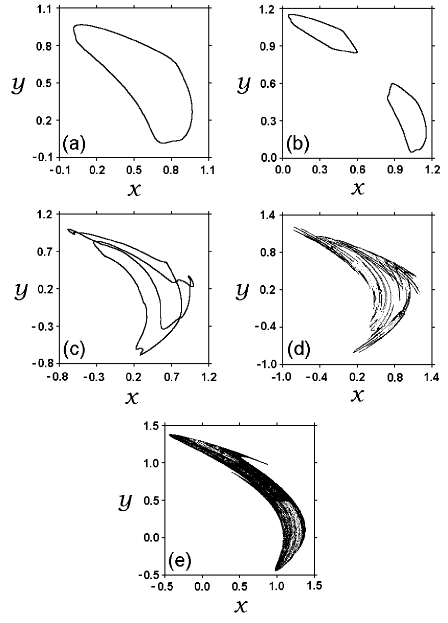
FIG. 1.: The typical attractors of the map (1): (a) torus T, (b) double torus 2T, (c) “double-wrapped” torus ${\rm T}_{2}$, (d) SNA, (e) chaotic attractor.

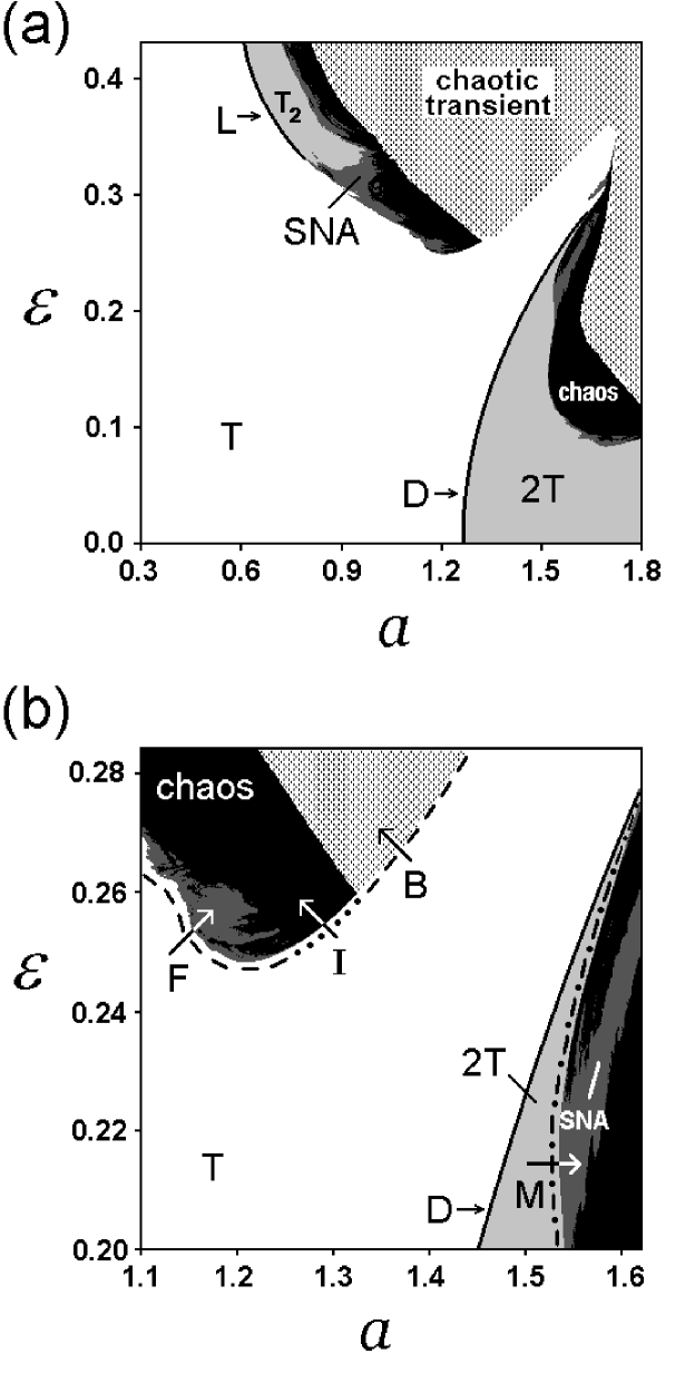
FIG. 2.: (a) The phase diagram of the map (1). (b) An enlarged fragment of the same diagram in the region of complex dynamical transitions.

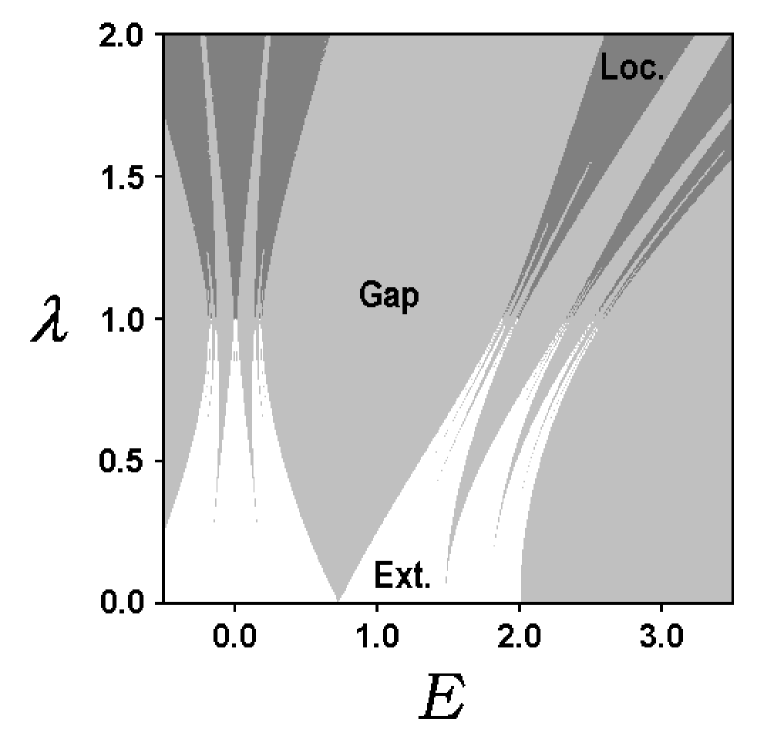
FIG. 3.: The phase diagram of the Harper equation with a quasiperiodic potential (17).

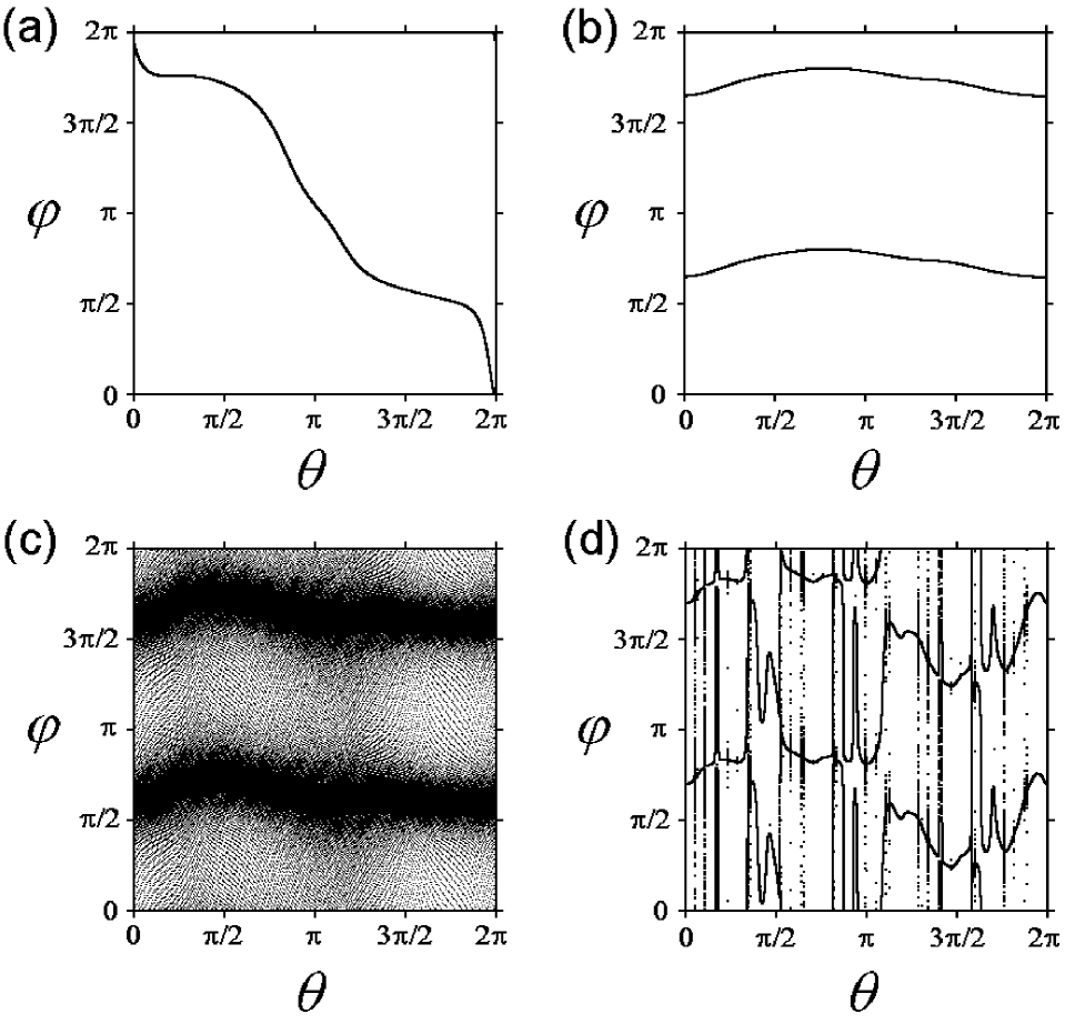
FIG. 4.: Attractors of the map (11) as graphic images of the dynamics of the perturbation angle $\varphi$: (a),(b)  two-frequency tori, (c) tree-frequency torus, (d) SNA.

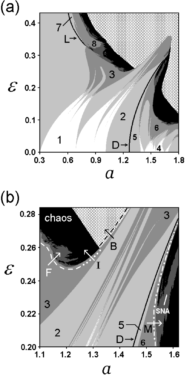
FIG. 5.: The combined phase diagram of the maps (1) and (11). See text of the Sec. V for details.

- [1] C. Grebogi, E. Ott, S. Pelikan, J. A. Yorke, Physica D 13, 261 (1984).
- [2] M. Ding, C. Grebogi, E. Ott, Phys. Lett. A 137, 167 (1989).
- [3] B. R. Hunt, E. Ott, Phys. Rev. Lett. 87, 254101 (2001).
- [4] J. Stark, Physica D 109, 163 (1997).
- [5] G. Keller, Fundamenta Mathematicae 151, 139 (1996).
- [6] S.P. Kuznetsov, A.S. Pikovsky, U. Feudel, Phys. Rev. E 51, R1629 (1995).
- [7] A. Pikovsky, U. Feudel, J. Phys. A: Math. Gen. 27, 5209 (1994).
- [8] A. S. Pikovsky, M. A. Zaks, U. Feudel, J. Kurths, Phys. Rev. E 52, 285 (1995).
- [9] U. Feudel, A. Pikovsky, A. Politi, J. Phys. A: Math. Gen. 29, 5297 (1996).
- [10] J. W. Shuai, K. W. Wong, Phys. Rev. E 57, 5332 (1998).
- [11] A. Pikovsky, U. Feudel, CHAOS 5, 253 (1995).
- [12] K. Kaneko, Prog. Theor. Phys. 69, 1806 (1983).
- [13] H. Broer, G. B. Huitema, F. Takens, B. L. J. Braaksma, Mem. Amer. Math. Soc. 83, 1 (1990).
- [14] P. R. Chastell, P. A. Glendinning, J. Stark, Phys. Lett. A 200, 17 (1995).
- [15] P. Glendinning, Discrete and Continuous Dynamical Systems - Series B Vol. 6, No 4, P. 1 (2002).
- [16] H. Daido, Prog. Theor. Phys. 71, 402 (1984).
- [17] U. Feudel, A. S. Pikovsky, J. Kurths, Physica D 88, 176 (1995).
- [18] H. Osinga, J. Wiersig, P. Glendinning, U. Feudel, Int. J. of Bifurcations and Chaos Vol. 11, No 12, P. 3085 (2001).
- [19] S. P. Kuznetsov, Phys. Rev. E 65, 066209 (2002).
- [20] T. Nishikawa, K. Kaneko, Phys. Rev. E 54, 6114 (1996).
- [21] S. Datta, R. Ramaswamy, A. Prasad, Phys. Rev. E 70, 046203 (2004).
- [22] J. F. Heagy, S. M. Hammel, Physica D 70, 140 (1994).
- [23] A. Prasad, V. Mehra, R. Ramaswamy, Phys. Rev. Lett. 79, 4127 (1997).
- [24] S.-Y. Kim, W. Lim, E. Ott, Phys. Rev. E 67, 056203 (2003).
- [25] T. Yalcinkaya, Y.-C. Lai, Phys. Rev. Lett. 77, 5039 (1996).
- [26] H. M. Osinga, U. Feudel, Physica D 141, 54 (2000).
- [27] S.-Y. Kim, W. Lim, Phys. Lett. A 334, 160 (2005).
- [28] O. Sosnovtseva, U. Feudel, J. Kurths, A. Pikovsky, Phys. Lett. A 218, 255 (1996).
- [29] J. Heagy, W. L. Ditto, J. Nonlinear Sci. 1, 423 (1991).
- [30] J. J. Stagliano, J.-M. Wersmger, E. E. Slaminka, Physica D 92, 164 (1996).
- [31] A. Witt, U. Feudel, A. S. Pikovsky, Physica D 109, 180 (1997).
- [32] A. Prasad, R. Ramaswamy, I. I. Satija, N. Shah, Phys. Rev. Lett. 83, 4530 (1999).
- [33] S. S. Negi, A. Prasad, R. Ramaswamy, Physica D 145, 1 (2000).
- [34] S. P. Kuznetsov, JETP Lett. 39, 113 (1984).
- [35] A. Yu. Jalnine, A. H. Osbaldestin, Phys. Rev. E 71, 016206 (2005).