Estimating von-Kármán’s constant from Homogeneous Turbulence

Abstract

A celebrated universal aspect of wall-bounded turbulent flows is the von Kármán log-law-of-the-wall, describing how the mean velocity in the streamwise direction depends on the distance from the wall. Although the log-law is known for more than 75 years, the von Kármán constant governing the slope of the log-law was not determined theoretically. In this Letter we show that the von-Kármán constant can be estimated from homogeneous turbulent data, i.e. without information from wall-bounded flows.

Introduction. The theoretical understanding of wall-bounded turbulent flows lags behind homogeneous turbulence, in which a number of universal constants and exponents can be estimated rather accurately on the basis of approximate arguments of considerable success Fri . One glaring such example of a lack of theoretical power concerns the apparently universal log law-of-the-wall which was discovered by von Kármán in 1930 79MY ; Pope . The law pertains to the mean velocity profile ${\bm{V}}(\bm{r})=\widehat{\bf{x}}\,V(\widehat{\bf{y}}\,y)$ in wall bounded Newtonian turbulence ($\widehat{\bf{x}}$, $\widehat{\bf{y}}$ and $\widehat{\bf{z}}$ are unit vectors in the stream-wise, wall-normal and span-wise directions respectively). In wall units the law is written as

$$V^{+}(y^{+})=\frac{1}{\kappa_{\rm K}}\ln y^{+}+B\,,\ \mbox{for}\ 30\leq y^{+}\ll Re_{\lambda}\ .$$ (1)

Here the Reynolds number ${{{\mathcal{R}}}\mkern-3.1mue}_{\lambda}$, the normalized distance from the wall $y^{+}$, and the normalized mean velocity $V^{+}(y^{+})$ (which is in the $\widehat{\bf{x}}$ direction with a dependence on $y$ only) are defined by

$${{{\mathcal{R}}}\mkern-3.1mue}_{\lambda}\equiv\frac{L\sqrt{\mathstrut p^{\prime}L}}{\nu_{0}}\,,\quad y^{+}\equiv\frac{y{{{\mathcal{R}}}\mkern-3.1mue}_{\lambda}}{L}\,,\quad V^{+}\equiv\frac{V}{\sqrt{\mathstrut p^{\prime}L}}\ .$$ (2)

Here $p^{\prime}$ be the fixed pressure gradients $p^{\prime}\equiv-\partial p/\partial x$, $\nu_{0}$ the kinematic viscosity. The law (1) is universal, independent of ${{{\mathcal{R}}}\mkern-3.1mue}_{\lambda}$, the nature of the Newtonian fluid and of the flow geometry over a smooth surface, providing that ${{{\mathcal{R}}}\mkern-3.1mue}_{\lambda}$  is large enough.

It is one of the shortcomings of the theory of wall-bounded turbulence that the von Kármán constant $\kappa_{\rm K}=0.44\pm 0.03$ and the intercept $B\approx 6.13$ are only known from experiments and simulations 79MY ; 97ZS . In this Letter we propose that $\kappa_{\rm K}$ can be estimated using universal constants that appear in homogenous turbulence. As such, we can draw on the relative power of homogeneous turbulence theory to improve our understanding of the characteristics of wall-bounded flows. We will not draw on any experimental information about wall-bounded flows.

In constructing our argument we rely heavily on known facts, including recent results, concerning homogeneous isotropic turbulence and homogeneous anisotropic turbulence with a constant shear: $\partial V(y)/\partial y=S$. Due to Galilean invariance the statistics of the turbulent velocity field ${{\bm{u}}}(\bm{r},t)$ (from which the mean $\left\langle{\bm{u}}(\bm{r},t)\right\rangle$ is subtracted) are independent of position. In other words, in such homogeneous and anisotropic ensemble all statistical object computed at any point, like the density of the kinetic energy $K$ and the Reynolds stress $W$,

$$K\equiv\left\langle|{\bm{u}}(\bm{r},t)|^{2}\right\rangle/2\,,\quad W\equiv-\left\langle u_{x}(\bm{r},t)u_{y}(\bm{r},t)\right\rangle\,,$$ (3)

are space independent. On the other hand, two-point correlation functions, like the second order longitudinal and transverse structure functions,

$$S_{2}({\bm{r}}) \equiv \big{\langle}\big{(}u_{\parallel}({\bm{r}}^{\prime}+{\bm{r}},t)-{\bm{u}}_{\parallel}({\bm{r}}^{\prime},t)\big{)}^{2}\big{\rangle}\,,$$ (4)

$$\widetilde{S}_{2}({\bm{r}}) \equiv \big{\langle}(u_{\perp}({\bm{r}}^{\prime}+{\bm{r}},t)-u_{\perp}({\bm{r}}^{\prime},t)\big{)}^{2}\big{\rangle}\,,$$ (5)

depend only on the vector separation $\bm{r}$. In Eq. (4) and (5) $u_{\parallel}$ and $u_{\perp}$ are components of ${\bm{u}}$, parallel and orthogonal to $\bm{r}$. The physical reason for the homogeneity of the turbulent statistics is that the energy flux $\varepsilon$ generated by the pressure head

$$\varepsilon=S\,W$$ (6)

is independent of the mean velocity itself (again, due to Galilean invariance) and is determined only by the space independent shear $S$ and Reynolds stress $W$.

I. Similarity of wall-bounded and constant-shear turbulence. We base our argument on the realization that wall-bounded turbulence in the log-law region and constant-shear turbulence are very similar. To be more precise, constant-shear homogeneous turbulence serves as a very good approximation to wall-bounded turbulence; various characteristics of turbulent statistics appear to coincide in the two flows within the available accuracy of physical experiments and numerical simulations. The basic reason for this similarity is precisely that the rate of the energy production  (6) depends on the shear itself and not on its space derivatives, which obviously differ in these two flows. The cenral point of this Letter is that the similarity between wall-bounded and constant-shear turbulence allows one to estimate the von-Kármán constant for wall-bounded turbulence using information from homogeneous constant-shear turbulence.

The first result that we quote is long standing, stating a universal relation between $W$ and $K$ in a constant-shear flow,

$$W\big{/}K\equiv W^{+}\big{/}K^{+}=c^{2}_{\rm N}\ ,\quad c_{\rm N}\approx 0.53\ .$$ (7)

The the same value of $c_{\rm N}$, within the available accuracy (of about 5%), is measured also in the outer layer of channel flow DNS . This serves as additional support for the similarity between these two types of turbulence.

Next we use the exact balance equation of mechanical momentum in a channel geometry,

$$\nu_{0}S(y)+W(y)=p^{\prime}(L-y)\ .$$ (8)

In wall units (2) this equation reads

$$S^{+}(y^{+})+W^{+}(y^{+})=1-y^{+}/{{{\mathcal{R}}}\mkern-3.1mue}_{\lambda}\ .$$ (9)

For ${{{\mathcal{R}}}\mkern-3.1mue}_{\lambda}\gg 1$ the mean shear $S^{+}$ in the log-law region (1) is governed by

$$S^{+}(y^{+})=1\big{/}(\kappa_{\rm K}\,y^{+})\,,$$ (10)

For large values of $y^{+}$ such that $y^{+}\ll{{{\mathcal{R}}}\mkern-3.1mue}_{\lambda}$ Eq. (9) reduces to

$$W^{+}=1\,,$$ (11)

meaning that in the log-law region the total momentum flux toward the wall is independent of the distance to the wall and is entirely accounted for by turbulent fluctuations (i.e. the Reynolds stress). Equations (7) and (11) show that in this region the kinetic energy is independent of the distance to the wall and has a universal value

$$K^{+}=c_{\rm N}^{-2}\ .$$ (12)

This constant value is shared by wall-bounded and constant-shear turbulence.

II. Anisotropy in wall-bounded and constant-shear turbulent flows. The knowledge of the total kinetic energy density (12) is not sufficient for our purposes, we need to know the distribution of $K$ between the different components of turbulent velocity, i.e. the values of

$$K_{x}\equiv\left\langle u_{x}^{2}\right\rangle/2\,,\quad K_{y}\equiv\left\langle u_{y}^{2}\right\rangle/2\,,\quad K_{z}\equiv\left\langle u_{z}^{2}\right\rangle/2\ .$$ (13)

The anisotropy of turbulent boundary layers, characterized by the dimensionless ratios $K_{j}/K$, plays an important role in various phenomena and was a subject of experimental and theoretical interest for many decades, see, e.g. 79MY ; Pope . Nevertheless, up to now the dispersion of results on this subject is too large. There is a widely spread opinion, based on old experiments, that the wall-normal turbulent fluctuations $K_{y}$ are much smaller than the other ones. For example, in the classical textbook by A.S. Monin and A.M. Yaglom 79MY it was reported that in a neutrally stratified log-boundary layer $K_{x}=0.54\,K$, $K_{y}=0.06\,K$ and $K_{z}=0.40\,K$. This appears to be in contradiction with simulation results at the largest Re_λ, ${{{\mathcal{R}}}\mkern-3.1mue}_{\lambda}$=590, which are available in Ref. DNS . These results are reproduced in Fig. 1. Note the region of $y^{+}$ values, about $100<y^{+}<\frac{2}{3}{{{\mathcal{R}}}\mkern-3.1mue}_{\lambda}$, where the plots of $K_{j}/K$ are nearly horizontal, as expected in the log-law region. From these plots we can conclude that is this region $K_{x}\approx 0.53\,K$ which is close to the ratio $0.54$, stated in 79MY . In contrast, the simulational data for $K_{y}/K$ and $K_{z}/K$ are completely different. From Fig. 1 one gets $K_{j}\approx 0.22\,K$ and $K_{z}\approx 0.27\,K$. Roughly speaking $K_{y}$ is almost equal to $K_{z}$. We propose that the difference between $K_{y}$ and $K_{z}$, observed in Fig. 1, is due to the effect of the spatial energy flux, that is expected to vanish in the asymptotic limit ${{{\mathcal{R}}}\mkern-3.1mue}_{\lambda}\to\infty$, but is still present at ${{{\mathcal{R}}}\mkern-3.1mue}_{\lambda}$ values available in direct numerical simulations DNS . Indeed, for both ${{{\mathcal{R}}}\mkern-3.1mue}_{\lambda}$ shown in Fig. 1 $K_{y}=K_{z}$ in the center of the channel, where the energy flux vanishes by symmetry. Clearly, there is no spatial energy flux also in a homogeneous constant shear turbulent flow. Based on the similarity between the wall bounded and constant shear turbulent flows we expect the values of $K^{+}_{i}$ to be the same for both flows in the limit ${{{\mathcal{R}}}\mkern-3.1mue}_{\lambda}\to\infty$. The expectation $K_{y}=K_{z}$ is confirmed by Large Eddy Simulation (LES) of a constant shear flow LES . As one sees in Fig. 2 in this flow $K_{x}\approx 0.46\,K$, while $K_{y}\approx K_{z}\approx 0.27\,K$. For both flows $K_{z}\approx 0.27\,K$, while in the stream-wise and and the wall-normal directions there is some difference in the ratios $K_{x}/K$ (0.53 vs. 0.46) and $K_{y}/K$ (0.22 vs. 0.27). We believe that these differences are again finite ${{{\mathcal{R}}}\mkern-3.1mue}_{\lambda}$ effects. This viewpoint is supported by a recent laboratory experiment by A. Agrawal, L. Djenidi and R.A. Antonia Exp in a vertical water channel with Re${}_{\lambda}=1000$ which is reproduced in Fig. 3. Indeed the experimental values of $K_{x}/K$, $K_{y}/K$ and $K_{z}/K$ distribute similarly to channel simulations and constant-shear LES:

$$K_{x}=K/2\,,\qquad K_{y}=K_{z}=K/4\ .$$ (14)

The operational conclusion of this discussion is that there are experimental and simulational grounds to believe that for both constant-shear and wall-bounded turbulent flows in the log-law region the turbulent kinetic energy is distributed in a very simple manner: the stream-wise component contains a half of total energy, the rest is equally distributed between wall-normal and cross-stream components. We propose that Eq. (14) is asymptotically exact.

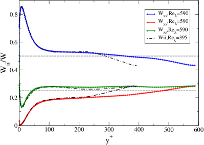
Figure 1: DNS profiles of the relative kinetic energies in the streamvise direction, $K_{x}/K$, lines denoted as “$xx$”, wall-normal, $K_{y}/K$, and spanwise, $K_{z}/K$, directions denoted as “$yy$” and “$zz$”. Solid lines: ${{{\mathcal{R}}}\mkern-3.1mue}_{\lambda}=590$, dot-dashed lines: ${{{\mathcal{R}}}\mkern-3.1mue}_{\lambda}=395$.

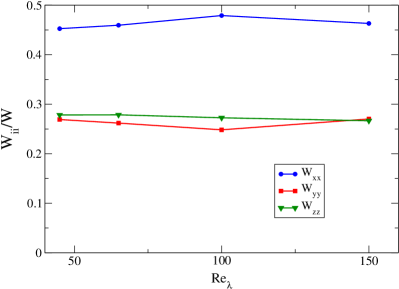
Figure 2: Relative components of the kinetic energies $K_{i}/K$ for for constant-shear flow. Results of the LES LES . Lines serve only to guide the eye.

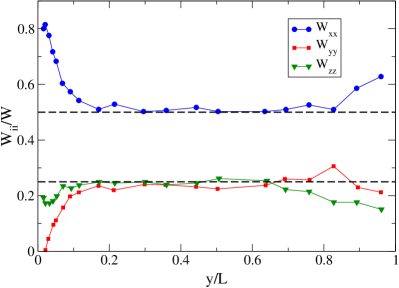
Figure 3: Experimental profiles of the relative kinetic energies in the vertical water channel with ${{{\mathcal{R}}}\mkern-3.1mue}_{\lambda}=1000$ according to Ref. Exp . Solid lines serve only to guide the eye. Dashed lines show the energy distribution (14).

III. Structure functions in isotropic, constant-shear, and wall bounded flows. In isotropic homogeneous turbulence the second order velocity structure functions, $S_{2}(\bm{r})$, [Eq. (4)] and $\widetilde{S}_{2}(\bm{r})$ [Eq. (5)] are very well studied. They are invariant to the direction of the separation vector ${\bm{r}}$ and up to intermittency corrections they read

$$S_{2}(r)=C_{2}(\epsilon r)^{\zeta_{2}}\,,\quad\widetilde{S}_{2}(r)=\widetilde{C}_{2}(\epsilon r)^{\zeta_{2}}\,,\quad\zeta_{2}=2/3\ .$$ (15)

The ratio of the dimensionless constants $\widetilde{C}_{2}/C_{2}=4/3$ follows from the incompressibly constraint, while the values of $\widetilde{C}_{2}$, $C_{2}$ are known from extensive experiments and simulationsFri ; 79MY :

$$\widetilde{C}_{2}=4\,C_{2}/3\,,\qquad C_{2}\approx 2.0\ .$$ (16)

For $r$ larger than the outer scale of turbulence, the correlations between velocities in $r$-separated points vanishes and the structure functions (15) saturate at their asymptotic values:

$$S_{2}(r)\to 2\big{<}u_{\parallel}^{2}\big{>}\,,\quad\widetilde{S}_{2}(r)\to 2\big{<}u_{\perp}^{2}\big{>}\ .$$ (17)

It is useful to define crossover scales $\ell_{2}$ and $\widetilde{\ell}_{2}$ for the longitudinal and transversal structure functions as follows:

$$S_{2}(\ell_{2})=2\big{<}u_{\parallel}^{2}\big{>}\,,\quad\widetilde{S}_{2}(\widetilde{\ell}_{2})=2\big{<}u_{\perp}^{2}\big{>}\ .$$ (18)

Clearly, in isotropic turbulence $\big{<}u_{\parallel}^{2}\big{>}=\big{<}u_{\perp}^{2}\big{>}$ and therefore the scales $\ell_{2}$ and $\widetilde{\ell}_{2}$ are related:

$$\widetilde{\ell}_{2}=\big{(}C_{2}\big{/}\widetilde{C}_{2}\big{)}^{3/2}\ell_{2}=3\sqrt{3}\,\ell_{2}/8\approx 0.65\,\ell_{2}\ .$$ (19)

The issue of the structure functions in anisotropic turbulent flows is considerably more involved 99ALP ; 05BP . In addition to the isotropic contribution (15), the structure functions have anisotropic components, $S_{2,j}$, belonging to irreducible representations of the SO(3) group with $j\neq 0$,

$$S_{2}(\bm{r})=\sum_{j=0}^{\infty}\sum_{m=-j}^{j}S^{(2)}_{jm}(\bm{r})$$ (20)

The various anisotropic sectors exhibit $\ell$ dependent scaling exponents:

$$S^{(2)}_{jm}(\bm{r})\propto r^{\zeta^{(2)}_{j}}Y_{jm}(\bm{r}/r)\,,$$ (21)

where the angular behavior of $S^{(2)}_{j,m}(\bm{r})$ is carried by the spherical harmonic $Y_{jm}(\bm{r}/r)$. The leading correction to the isotropic sector  (15) is given the $j=2$ contribution with $\zeta^{(2)}_{2}\approx\frac{4}{3}$. The mixture of contributions with different different exponents, each with an amplitude that depends on the distance to the wall, may give the false impression that the scaling exponents of $S_{2}$ and $\widetilde{S}_{2}$ are different; this impression disappears once the structure functions are projected on the various sectors of the symmetry group, where their exponents are the same (appearing universal) , but their amplitudes are of course non-universal, and see full details in 05BP .

Importantly, all the anisotropic contributions (21) can be eliminated by averaging over all the directions of $\bm{r}$ because

$$\int Y_{jm}\left(\bm{r}/r\right)d(\bm{r}/r)=0\,,\quad\mbox{for}\ j\neq 0\ .$$ (22)

After the elimination of the anisostropic sectors, the isotropic parts of $S_{2}(\bm{r})$, $\widetilde{S}_{2}(\bm{r})$, i.e. $S_{2,0}(\bm{r})$, $\widetilde{S}_{2,0}(\bm{r})$ exhibit the same scaling behavior as structure functions in isotropic turbulence, even in relatively low ${{{\mathcal{R}}}\mkern-3.1mue}_{\lambda}$ channel flows 99ABMP . The situation for high ${{{\mathcal{R}}}\mkern-3.1mue}_{\lambda}$ constant-shear and wall-bounded turbulence is even simpler. As demonstrated by Eq. (14), in these flows only the streamwise direction $\widehat{\bf{x}}$ is special, the partial kinetic energies in two other directions are equal: $K_{z}=K_{y}$. Therefore in the limit ${{{\mathcal{R}}}\mkern-3.1mue}_{\lambda}\to\infty$ the symmetry of these two flows can be considered as axisymmetric with the axis in the $\widehat{\bf{x}}$ direction, and one can eliminate the anisotropic contributions by averaging only in the $(\widehat{\bf{x}},\widehat{\bf{z}})$-plane, parallel to the wall.

This idea is supported by experiments in the atmospheric turbulent boundary layer 00KLPS ), in which the ground normal velocity component $u_{y}$ was measured at point of fixed height $y$ above the ground, separated by ${\bm{\rho}}$ which was parallel to the ground. Denote the resulting structure function as $\widetilde{S}_{2}(y,{\bm{\rho}})$. After averaging over the azimuthal angle $\phi$ in the $(\widehat{\bf{x}},\widehat{\bf{z}})$-plane, this function exhibits homogeneous scaling behavior (15) for all scales up to separations $\rho$ in the $(\widehat{\bf{x}},\widehat{\bf{z}})$-plane which are close to the wall distance $y$:

$$\left\langle\widetilde{S}_{2}(y,\rho)\right\rangle_{\phi}=\widetilde{C}_{2}(\epsilon\rho)^{2/3}\,,\quad\rho\leq y\ .$$ (23)

The constant $\widetilde{C}_{2}$ here is the same as in isotropic turbulence. Inspired by this experiment (and see Fig. 3 in Ref. 00KLPS ) we make the assumption that the largest of the two crossover scales (18), namely $\ell_{2}$, is determined by the distance to the wall:

$$\ell_{2}=y\ .$$ (24)

In other words, the assumption is that the structure function $\left\langle\widetilde{S}_{2}(y,\rho)\right\rangle_{\phi}$ changes sharply from a scaling law in $\rho$ to its asymptotic constant value precisely at $\rho=y$. This assumption introduces an unknown factor of the order of unity to our arguments; we take this factor to be exactly unity.

Relationship between $C_{2}$, $c_{\rm N}$ and $\kappa_{\rm K}$. We have presented all the ingredients necessary to estimate the von Kármán constant. This constant will be related to the Kolmogorov constant $C_{2}$ which appears in homogeneous isotropic flows and to the ratio $c_{\rm N}$ which appears in homogeneous constant shear flows. Using Eqs, (14), (18), (19) and (24) in Eq. (23) one gets:

$$K=4K_{y}=2\left\langle u_{y}^{2}\right\rangle=\widetilde{C}_{2}(\epsilon\widetilde{\ell}_{2})^{2/3}=C_{2}(\epsilon y)^{2/3}\ .$$ (25)

In wall units $K^{+}=C_{2}(\epsilon^{+}y^{+})^{2/3}$. Taking $\epsilon$ from Eq. (6) and $K^{+}$ from Eq. (12) we have

$$c_{\rm N}^{-2}=C_{2}\,(S^{+}W^{+}y^{+})^{2/3}\ .$$ (26)

Together with Eqs. (10) and (11) this leads to the relationship:

$$\kappa_{\rm K}=\left(\,c_{\rm N}\sqrt{C_{2}}\,\right)^{3}\ .$$ (27)

Using the experimental values $c_{\rm N}\approx 0.53$ and $C_{2}\approx 2.0$ we get $\kappa_{\rm N}\approx 0.42$ in excellent agreement with the known value of this constant, $\kappa_{\rm N}\approx 0.44\pm 0.03$. It should be stressed that in fact we have used only one assumption (24) about the cross-over scale of the structure function. All the other input is taken from homogeneous data without any wall in sight. We propose that the numerical agreement with known value of $\kappa_{\rm K}$ reflects the quality of the input values of $C_{2}$ and $c_{\rm N}$.

- (1) U. Frisch, Turbulence, the legacy of A.N. Kolmogorov, (Cambridge, 1995).
- (2) A. S. Monin and A. M. Yaglom, Statistical Fluid Mechanics (MIT, 1979, vol. 1 chapter 3).
- (3) S. B. Pope, Turbulent Flows, University Press, (Cambridge, 2000).
- (4) M.V. Zagarola and A.J. Smits, Phys. Rev. Lett. 78, 239 (1997).
- (5) R.B. Bird, C.F. Curtiss, R.C. Armstrong, O. Hassager, Dynamics of Polymeric Fluids (Wiley, NY 1987).
- (6) V. S. L’vov, A. Pomyalov and V. Tiberkevich, “Simple analytical model for entire turbulent boundary layer over flat plane”, Environmental Fluid Mechanics, in press, (2005). Also:nlin.CD/0404010.
- (7) Moser, R. G., Kim, J., and Mansour, N. N.: 1999, Direct numerical simulation of turbulent channel flow up to , Phys. Fluids 11, 943; DNS data at http://www.tam.uiuc.edu/Faculty/Moser/channel.
- (8) C. M. Casciola, pivate communication.
- (9) A. Agrawal, L. Djenidi and R.A. Antonia, “Evolution of the anisotropy over a fla plane with suction”, 12th International symposium on application of the laser technology to fluid mechanics, Lisbon, Portugal, July 2004. Available at URL http://in3.dem.ist.utl.pt/lxlaser2004/pdf/paper_28_1.pdf
- (10) I. Arad, V. S. L’vov and I. Procaccia. PRE 59, 6753 (1999)
- (11) L. Biferale and I. Procaccia, Phys. Rep. 414, 43 2005, and references therein.
- (12) I. Arad, L. Biferale, I. Mazzitelli and I. Procaccia, Phys. Rev. Lett. 82, 5040 (1999)
- (13) S. Kurien, V.S. L’vov, I. Procaccia, K.R. Sreenivasan, Phys. Rev. E, 61, 407-421 (2000).