Chaotic Dynamics of N–degree of Freedom Hamiltonian Systems

Abstract

We investigate the connection between local and global dynamics of two $N$–degree of freedom Hamiltonian systems with different origins describing one–dimensional nonlinear lattices: The Fermi–Pasta–Ulam (FPU) model and a discretized version of the nonlinear Schrödinger equation related to the Bose–Einstein Condensation (BEC). We study solutions starting in the immediate vicinity of simple periodic orbits (SPOs) representing in–phase (IPM) and out–of–phase motion (OPM), which are known in closed form and whose linear stability can be analyzed exactly. Our results verify that as the energy $E$ increases for fixed $N$, beyond the destabilization threshold of these orbits, all positive Lyapunov exponents $L_{i},\ i=1,\ldots,N-1$, exhibit a transition between two power laws, $L_{i}\propto E^{B_{k}}$, $B_{k}>0,\ k=1,2$, occurring at the same value of $E$. The destabilization energy $E_{c}$ per particle goes to zero as $N\rightarrow\infty$ following a simple power–law, $E_{c}/N\propto N^{-\alpha}$, with $\alpha$ being 1 or 2 for the cases we studied. However, using the SALI, a very efficient indicator we have recently introduced for distinguishing order from chaos, we find that the two Hamiltonians have very different dynamics near their stable SPOs: For example, in the case of the FPU system, as the energy increases for fixed $N$, the islands of stability around the OPM decrease in size, the orbit destabilizes through period–doubling bifurcation and its eigenvalues move steadily away from $-1$, while for the BEC model the OPM has islands around it which grow in size before it bifurcates through symmetry breaking, while its real eigenvalues return to $+1$ at very high energies. Furthermore, the IPM orbit of the BEC Hamiltonian never destabilizes, having finite–sized islands around it, even for very high $N$ and $E$. Still, when calculating Lyapunov spectra, we find for the OPMs of both Hamiltonians that the Lyapunov exponents decrease following an exponential law and yield extensive Kolmogorov–Sinai entropies per particle $h_{KS}/N\propto\mathrm{const.}$, in the thermodynamic limit of fixed energy density $E/N$ with $E$ and $N$ arbitrarily large.

¹Department of Mathematics
and
Center for Research and Applications of Nonlinear Systems (CRANS),
University of Patras,
GR–$26500$, Rio, Patras, Greece
²Research Center for Astronomy and Applied Mathematics
Academy of Athens,
Soranou Efesiou $4$, GR–$11527$, Athens, Greece
³Department of Applications of Informatics and Management in Finance,
Technological Institute of Mesologhi,
GR–$30200$, Mesologhi, Greece

Keywords: Hamiltonian systems, Simple Periodic Orbits, regular and chaotic behavior, Lyapunov spectra, Kolmogorov entropy, SALI method.

1 Introduction

Chaotic behavior in Hamiltonian systems with many degrees of freedom has been the subject of intense investigation in the last fifty years, see e.g. [Lichtenberg & Lieberman, 1991; MacKay & Meiss, 1987; Wiggins, 1988] and Simó ed., [1999]. By degrees of freedom (dof) we are referring to the number of canonically conjugate pairs of positions and momentum variables, $q_{k}$ and $p_{k}$ respectively, with $k=1,2,\ldots,N$. The relevance of these systems to problems of practical concern cannot be overemphasized. Their applications range from the stability of the solar system Contopoulos, [2002] and the containment of charged particles in high intensity magnetic fields Lichtenberg & Lieberman, [1991] to the blow–up of hadron beams in high energy accelerators Scandale & Turchetti, eds. [1991] and the understanding of the properties of simple molecules and hydrogen–bonded systems Bountis ed., [1992]; Prosmiti & Farantos, [1995].

One of the most fundamental areas in which the dynamics of multi–degree of freedom Hamiltonian systems has played (and continues to play) a crucial role is the study of transport phenomena in one–dimensional ($1$D) lattices and the role of chaos in providing a link between deterministic and statistical behavior Chirikov, [1979]; Lichtenberg & Lieberman, [1991]; Ford, [1992]. In this context, a lattice of $N$ dof is expected, in the thermodynamic limit ($N\rightarrow\infty$ at fixed energy density $E/N$) to exhibit chaotic behavior for almost all initial configurations, satisfying at least the property of ergodicity. This would allow the use of probability densities, leading from the computation of orbits to the study of statistical quantities like ensemble averages and transport coefficients.

Chaotic regions, where nearby solutions diverge exponentially from each other, provide an excellent “stage” on which such a desired transition from classical to statistical mechanics can occur. However, the presence of significantly sized islands (or tori) of quasiperiodic motion, in which the dynamics is “stable” for long times, preclude the success of this scenario and make any attempt at a globally valid statistical description seriously questionable. These tori occur e.g. around simple periodic orbits which are stable under small perturbations and, if their size does not shrink to zero as $N$ or $E$ increases, their presence can attribute global consequences to a truly local phenomenon.

That such important periodic orbits do exist in Hamiltonian lattices, even in the $N\rightarrow\infty$ limit, could not have been more dramatically manifested than in the remarkable discovery of discrete breathers (see e.g. Flach & Willis, [1998]), which by now have been observed in a great many experimental situations [Eisenberg et al., 1998; Schwarz et al., 1999; Fleischer et al., 2003; Sato et al., 2003]. Discrete breathers are precisely one such kind of stable periodic orbits, which also happen to be localized in space, thus representing a very serious limitation to energy transport in nonlinear lattices.

Then, there were, of course, the famous numerical experiments of Fermi, Pasta and Ulam of the middle $1950$’s Fermi et al., [1955], which demonstrated the existence of recurrences that prevent energy equipartition among the modes of certain $1$D lattices, containing nonlinear interactions between nearest neighbors. These finite, so–called FPU Hamiltonian systems were later shown to exhibit a transition to “global” chaos, at high enough energies where major resonances overlap Izrailev & Chirikov, [1966]. Before that transition, however, an energy threshold to a “weak” form of chaos was later discovered that relies on the interaction of the first few lowest frequency modes and, at least for the FPU system, does appear to ensure equipartition among all modes [De Luca et al., $1995$; De Luca & Lichtenberg, $2002$]. Interestingly enough, very recently, this transition to “weak” chaos was shown to be closely related to the destabilization of one of the lowest frequency nonlinear normal mode of this FPU system Flach et al., [2005]. Thus, today, $50$ years after its famous discovery, the Fermi–Pasta–Ulam problem and its transition from recurrences to true statistical behavior is still a subject of ongoing investigation Berman & Izrailev, [2004].

In this paper, we have sought to approach the problem of global chaos in Hamiltonian systems, by considering two paradigms of $N$ dof, $1$D nonlinear lattices, with very different origins.

One is the famous FPU lattice mentioned above, with quadratic and quartic nearest neighbor interactions, described by the Hamiltonian

$$H=\frac{1}{2}\sum_{j=1}^{N}\dot{x}_{j}^{2}+\sum_{j=0}^{N}\biggl{(}\frac{1}{2}(x_{j+1}-x_{j})^{2}+\frac{1}{4}\beta(x_{j+1}-x_{j})^{4}\biggr{)}=E$$ (1)

where $x_{j}$ is the displacement of the $j$th particle from its equilibrium position, $\dot{x}_{j}$ is the corresponding canonically conjugate momentum of $x_{j}$, $\beta$ is a positive real constant and $E$ is the value of the Hamiltonian representing the total energy of the system.

The other one is obtained by a discretization of a partial differential equation (PDE) of the nonlinear Schrödinger type referred to as the Gross–Pitaevskii equation Dalfovo et al., [1999], which in dimensionless form reads

$$i\hslash\frac{\partial\Psi(x,t)}{\partial t}=-\frac{\hslash^{2}}{2}\frac{\partial^{2}\Psi(x,t)}{\partial x^{2}}+V(x)\Psi(x,t)+g|\Psi(x,t)|^{2}\Psi(x,t),\ i^{2}=-1$$ (2)

where $\hslash$ is the Planck constant, $g$ is a positive constant (repulsive interactions between atoms in the condensate) and $V(x)$ is an external potential.

Equation (2) is related to the phenomenon of Bose–Einstein Condensation (BEC) Ketterle et al., [1999]. Here we consider the simple case $V(x)=0$, $\hslash=1$ and discretize the $x$–dependence of the complex variable $\Psi(x,t)\equiv\Psi_{j}(t)$ in (2), approximating the second order derivative by $\Psi_{xx}\simeq\frac{\Psi_{j+1}+\Psi_{j-1}-2\Psi_{j}}{\delta x^{2}}$. Setting then $\Psi_{j}(t)=q_{j}(t)+i\cdot p_{j}(t),\ i^{2}=-1,\;j=1,2,\ldots,N$ and $|\Psi(x,t)|^{2}=q_{j}^{2}(t)+p_{j}^{2}(t)$, one immediately obtains from the above PDE (2) a set of ordinary differential equations (ODEs) for the canonically conjugate variables, $p_{j}$ and $q_{j}$, described by the BEC Hamiltonian Trombettoni & Smerzi, [2001]; Smerzi & Trombettoni, [2003]

$$H=\frac{1}{2}\sum_{j=1}^{N}(p_{j}^{2}+q_{j}^{2})+\frac{\gamma}{8}\sum_{j=1}^{N}(p_{j}^{2}+q_{j}^{2})^{2}-\frac{\epsilon}{2}\sum_{j=1}^{N}(p_{j}p_{j+1}+q_{j}q_{j+1})=E$$ (3)

where $\gamma>0$ and $\epsilon=1$ are constant parameters, $g=\frac{\gamma}{2}>0$ with $\delta x=1$ and $E$ is the total energy of the system.

In Sec. 2, we study these Hamiltonians, focusing on some simple periodic orbits (SPOs), which are known in closed form and whose local (linear) stability analysis can be carried out to arbitrary accuracy. By SPOs, we refer here to periodic solutions where all variables return to their initial state after only one maximum and one minimum in their oscillation, i.e. all characteristic frequencies have unit ratios. In particular, we examine first their bifurcation properties to determine whether they remain stable for arbitrarily large $E$ and $N$, having perhaps finitely sized islands of regular motion around them. This was found to be true only for the so–called in–phase–mode (IPM) of the BEC Hamiltonian (3).

SPOs corresponding to out–of–phase motion (OPM) of either the FPU (1) or the BEC system (3) destabilize at energy densities $\frac{E_{c}}{N}\propto N^{-\alpha}$, with $\alpha=1$ or $2$ (for the SPOs we studied), as $N\rightarrow\infty$. The same result was also obtained for what we call the OHS mode of the FPU system Ooyama et al., [1969], where all even indexed particles are stationary and all others execute out–of–phase oscillation, under fixed or periodic boundary conditions. All these are in agreement with detailed analytical results obtained for families of SPOs of the same FPU system under periodic boundary conditions (see e.g. Poggi & Ruffo, [1997]).

Then, in Sec. 3, we vary the values of $E$ and $N$ and study the behavior of the Lyapunov exponents of the OPMs of the FPU and BEC Hamiltonians. We find that, as the eigenvalues of the monodromy matrix exit the unit circle on the real axis, at energies $0<E_{c}\equiv E_{1}<E_{2}<\ldots$, for fixed $N$, all positive Lyapunov exponents $L_{i},\ i=1,\ldots,N-1$, increase following two distinct power laws, $L_{i}\propto E^{B_{k}}$, $B_{k}>0,\ k=1,2$, with the $B_{k}$’s as reported in the literature, Rechester et al., [1979]; Benettin, [1984] and Livi et al., [1986]. Furthermore, as the energy $E$ grows at fixed $N$, the real eigenvalues of the OPM orbit of FPU continue to move away from $-1$, unlike the OPM of the BEC Hamiltonian, where for very large $E$ all these eigenvalues tend to return to $+1$. Interestingly enough, the IPM of the BEC Hamiltonian remains stable for all the energies and number of dof we studied!

In Sec. 4, we turn to the question of the “size” of islands around stable SPOs and use the Smaller Alignment Index (SALI), introduced in earlier papers Skokos, [2001]; Skokos et al., 2003a ; Skokos et al., 2003b ; Skokos et al., [2004] to distinguish between regular and chaotic trajectories in our two Hamiltonians. First, we verify again in these multi–degree of freedom systems the validity of the SALI dependence on the two largest Lyapunov exponents $L_{1}$ and $L_{2}$ in the case of chaotic motion, to which it owes its effectiveness and predictive power. Then, computing the SALI, at points further and further away from stable SPOs, we determine approximately the “magnitude” of these islands and find that it vanishes (as expected) at the points where the corresponding OPMs destabilize. In fact, for the OPM of the FPU system the size of the islands decreases monotonically before destabilization while for the BEC orbit the opposite happens! Even more remarkably, for the IPM of the BEC Hamiltonian (3), not only does the “size” of the island not vanish, it even grows with increasing energy and remains of considerable magnitude for all the values of $E$ and $N$ we considered.

Finally, in Sec. 5, using as initial conditions the unstable SPOs, we compute the Lyapunov spectra of the FPU and BEC systems in the so–called thermodynamic limit, i.e. as the energy $E$ and the number of dof $N$ grow indefinitely, with energy density $\frac{E}{N}$ fixed. First, we find that Lyapunov exponents, fall on smooth curves of the form $L_{i}\approx L_{1}e^{-\alpha i/N}$, for both systems. Then, computing the Kolmogorov–Sinai entropy $h_{KS}$, as the sum of the positive Lyapunov exponents Pesin, [1976]; Hilborn, [1994], in the thermodynamic limit, we find, for both Hamiltonians, that $h_{KS}$ is an extensive quantity as it grows linearly with $N$, demonstrating that in their chaotic regions the FPU and BEC Hamiltonians behave as ergodic systems of statistical mechanics.

2 Simple Periodic Orbits (SPOs) and Local Stability Analysis

2.1 The FPU model

2.1.1 Analytical expressions of the OHS mode

We consider a $1$D lattice of $N$ particles with nearest neighbor interactions given by the Hamiltonian Fermi et al., [1955]

$$H=\frac{1}{2}\sum_{j=1}^{N}\dot{x}_{j}^{2}+\sum_{j=0}^{N}\biggl{(}\frac{1}{2}(x_{j+1}-x_{j})^{2}+\frac{1}{4}\beta(x_{j+1}-x_{j})^{4}\biggr{)}$$ (4)

where $x_{j}$ is the displacement of the $j$th particle from its equilibrium position, $\dot{x}_{j}$ is the corresponding canonically conjugate momentum of $x_{j}$ and $\beta$ is a positive real constant.

Imposing fixed boundary conditions

$$x_{0}(t)=x_{N+1}(t)=0,\;\forall t$$ (5)

one finds a simple periodic orbit first studied by Ooyama et al., [1969], taking $N$ odd, which we shall call the OHS mode (using Ooyama’s, Hirooka’s and Saitô’s initials)

$$\hat{x}_{2j}(t)=0,\;\hat{x}_{2j-1}(t)=-\hat{x}_{2j+1}(t)\equiv\hat{x}(t),\;j=1,\ldots,\frac{N-1}{2}.$$ (6)

Here, we shall examine analytically the stability properties of this mode and determine the energy range $0\leq E\leq E_{c}(N)$ over which it is linearly stable.

The equations of motion associated with Hamiltonian (4) are

$$\ddot{x}_{j}(t)=x_{j+1}-2x_{j}+x_{j-1}+\beta\Bigl{(}(x_{j+1}-x_{j})^{3}-(x_{j}-x_{j-1})^{3}\Bigr{)},\;j=1,\ldots,N$$ (7)

whence, using the boundary condition (5) and the expressions (6) for every $j=1,3,\ldots,N-2,N$, we arrive at a single equation

$$\ddot{\hat{x}}(t)=-2\hat{x}(t)-2\beta\hat{x}^{3}(t)$$ (8)

describing the anharmonic oscillations of all odd particles of the initial lattice. The solution of (8) is, of course, well–known in terms of Jacobi elliptic functions Abramowitz & Stegun, [1965] and can be written as

$$\hat{x}(t)=\mathcal{C}\mathop{\operator@font cn}(\lambda t,{\kappa}^{2})$$ (9)

where

$$\mathcal{C}^{2}=\frac{2{\kappa}^{2}}{\beta(1-2{\kappa}^{2})},\ \lambda^{2}=\frac{2}{1-2{\kappa}^{2}}$$ (10)

and ${\kappa}^{2}$ is the modulus of the $\mathop{\operator@font cn}$ elliptic function. The energy per particle of this SPO is then given by

$$\frac{E}{N+1}=\frac{1}{4}\mathcal{C}^{2}(2+\mathcal{C}^{2}\beta)=\frac{{\kappa}^{2}-{\kappa}^{4}}{(1-2{\kappa}^{2})^{2}\beta}.$$ (11)

2.1.2 Stability analysis of the OHS mode

Setting $x_{j}=\hat{x}_{j}+y_{j}$ in (7) and keeping up to linear terms in $y_{j}$ we get the corresponding variational equations for the OHS mode (6)

$$\ddot{y}_{j}=(1+3\beta\hat{x}^{2})(y_{j-1}-2y_{j}+y_{j+1}),\;j=1,\ldots,N$$ (12)

where $y_{0}=y_{N+1}=0$.

Using the standard method of diagonalization of linear algebra, we can separate these variational equations to $N$ uncoupled independent Lamé equations [Abramowitz & Stegun, 1965]

$$\ddot{z}_{j}(t)+4(1+3\beta\hat{x}^{2}){\sin}^{2}\biggl{(}\frac{\pi j}{2(N+1)}\biggr{)}z_{j}(t)=0,\;j=1,\ldots,N$$ (13)

where the $z_{j}$ variations are simple linear combinations of $y_{j}$’s. Using (9) and changing variables to $u=\lambda t$, Eq. (13) takes the form

$${z_{j}^{\prime\prime}}(u)+2\bigl{(}1+4{\kappa}^{2}-6{\kappa}^{2}{\mathop{\operator@font sn}}^{2}(u,{\kappa}^{2})\bigr{)}{\sin}^{2}\biggl{(}\frac{\pi j}{2(N+1)}\biggr{)}z_{j}(u)=0,\;j=1,\ldots,N$$ (14)

where we have used the identity ${\mathop{\operator@font cn}}^{2}(u,{\kappa}^{2})=1-{\mathop{\operator@font sn}}^{2}(u,{\kappa}^{2})$ and primes denote differentiation with respect to $u$.

Equation (14) is an example of Hill’s equation [Copson, $1935$; Magnus & Winkler, $1966$]

$${z^{\prime\prime}}(u)+Q(u)z(u)=0$$ (15)

where $Q(u)$ is a $T$–periodic function ($Q(u)=Q(u+T)$) with $T=2\mathcal{K}$ and $\mathcal{K}\equiv\mathcal{K}(\kappa^{2})$ is the elliptic integral of the first kind.

According to Floquet theory Magnus & Winkler, [1966] the solutions of Eq. (15) are bounded (or unbounded) depending on whether the Floquet exponent $\alpha$, given by

$$\cos\Bigl{(}2\alpha\mathcal{K}(\kappa^{2})\Bigr{)}=1-2{\sin}^{2}\Bigl{(}\mathcal{K}(\kappa^{2})\sqrt{a_{0}}\Bigr{)}\det\Bigl{(}\mathbf{D}(0)\Bigr{)}$$ (16)

is real (or imaginary). The matrix $\mathbf{D}(\alpha)$ is called Hill’s matrix and in our case its entries are given by

$$[\mathbf{D}(\alpha)]_{n,m}\equiv\frac{a_{n-m}}{a_{0}-\Bigl{(}\alpha+\frac{n\pi}{\mathcal{K}(\kappa^{2})}\Bigr{)}^{2}}+\delta_{n,m}$$ (17)

where $\delta_{n,m}=\begin{cases}1,&n=m\cr 0,&n\neq m\cr\end{cases}$, is the Kronecker delta with $n$, $m\in\mathbb{Z}$ and the $a_{n}$’s are the coefficients of the Fourier series expansion of $Q(u)$,

$$Q(u)=\sum_{n=-\infty}^{\infty}a_{n}e^{\frac{in\pi u}{\mathcal{K}(\kappa^{2})}}.$$ (18)

Thus, Eq. (16) gives a stability criterion for the OHS mode (6), by the condition

$$\Bigl{|}1-2{\sin}^{2}\Bigl{(}\mathcal{K}(\kappa^{2})\sqrt{a_{0}}\Bigr{)}\det\Bigl{(}\mathbf{D}(0)\Bigr{)}\Bigr{|}=\begin{cases}<1,&\mathrm{stable\;mode}\cr>1,&\mathrm{unstable\;mode}\end{cases}.$$ (19)

In this case, the Fourier coefficients of Hill’s matrix $\mathbf{D}(0)$ are given by the relations [Copson, $1935$]

$$a_{0} = 2\Biggr{(}-5+4\kappa^{2}+6\frac{\mathcal{E}(\kappa^{2})}{\mathcal{K}(\kappa^{2})}\Biggl{)}{\sin}^{2}\Biggl{(}\frac{\pi j}{2(N+1)}\Biggl{)}$$ (20)

$$a_{n} = 2\frac{6n\pi^{2}q^{n}}{\mathcal{K}^{2}(\kappa^{2})(1-q^{2n})}{\sin}^{2}\Biggl{(}\frac{\pi j}{2(N+1)}\Biggl{)},\;n\neq 0$$ (21)

where $q\equiv e^{-\pi\frac{\mathcal{K}^{\prime}}{\mathcal{K}}}$, $\mathcal{K}\equiv\mathcal{K}(\kappa^{2})$ and $\mathcal{E}\equiv\mathcal{E}(\kappa^{2})$ are the elliptic integrals of the first and second kind respectively and $\mathcal{K}^{\prime}\equiv\mathcal{K}(\kappa^{\prime 2})$ with $\kappa^{\prime 2}\equiv 1-\kappa^{2}$.

In the evaluation of $\mathbf{D}(0)$ in Eq. (19) we have used $121$ terms in the Fourier series expansion of $\mathop{\operator@font sn}^{2}(u,\kappa^{2})$ (that is, $121\times 121$ Hill’s determinants of $\mathbf{D}(0)$). Thus, we determine with accuracy $10^{-8}$ the $\kappa^{2}\equiv\kappa^{2}_{j}$ values at which the Floquet exponent $\alpha$ in (16) becomes zero and the $z_{j}(u)$ in (14) become unbounded. We thus find that the first variation $z_{j}(u)$ to become unbounded as $\kappa^{2}$ increases is $j=\frac{N-1}{2}$ and the energy values $E_{c}$ at which this happens (see Eq. (11)) are listed in Table 1 for $\beta=1.04$. The $z_{j}(u)$ variation with $j=\frac{N+1}{2}$ has Floquet exponent $\alpha$ equal to zero for every $\kappa^{2}\in[0,\frac{1}{2}]$, that is $z_{\frac{N+1}{2}}(u)$ corresponds to variations along the orbit.

$N$	$5$	$7$	$9$	$11$	$13$	$15$
$E_{c}$	6.4932	3.0087	2.2078	1.8596	1.6669	1.5452

Table 1: The energies $E_{c}$, for $\beta=1.04$, at which the $z_{\frac{N-1}{2}}(u)$ in (14) becomes unbounded for some odd values of $N$.

Next we vary $N$ and calculate the destabilization energy per particle $\frac{E_{c}}{N}$ for $\beta=1.04$ at which the OHS nonlinear mode (6) becomes unstable. Plotting the results in Fig. 1, we see that $\frac{E_{c}}{N}$ decreases for large $N$ with a simple power–law, as $1/N$.

Figure 1: The solid curve corresponds to the energy per particle $\frac{E_{c}}{N}$, for $\beta=1.04$, of the first destabilization of the OHS nonlinear mode (6) of the FPU system (4) obtained by the numerical evaluation of the Hill’s determinant in (19), while the dashed line corresponds to the function $\propto\frac{1}{N}$. Note that both axes are logarithmic.

2.1.3 Analytical study of an OPM solution

We now turn to the properties of another SPO of the FPU Hamiltonian (4), studied in Budinsky & Bountis, [1983]; Poggi & Ruffo, [1997] and [Cafarella et al., 2003]. In particular, imposing the periodic boundary conditions

$$x_{N+1}(t)=x_{1}(t),\;\forall t$$ (22)

with $N$ even, we analyze the stability properties of the out–of–phase mode (OPM) defined by

$$\hat{x}_{j}(t)=-\hat{x}_{j+1}(t)\equiv\hat{x}(t),\;j=1,\ldots,N.$$ (23)

In this case the equations of motion (7) reduce also to a single differential equation

$$\ddot{\hat{x}}(t)=-4\hat{x}(t)-16\beta\hat{x}^{3}(t)$$ (24)

describing the anharmonic oscillations of all particles of the initial lattice. The solution of Eq. (24) can again be written as an elliptic $\mathop{\operator@font cn}$–function

$$\hat{x}(t)=\mathcal{C}\mathop{\operator@font cn}(\lambda t,{\kappa}^{2})$$ (25)

with

$$\mathcal{C}^{2}=\frac{{\kappa}^{2}}{2\beta(1-2{\kappa}^{2})},\ \ \ \lambda^{2}=\frac{4}{1-2{\kappa}^{2}}.$$ (26)

The energy per particle of the nonlinear OPM (23) is given by

$$\frac{E}{N}=2\mathcal{C}^{2}(1+2\mathcal{C}^{2}\beta)=\frac{{\kappa}^{2}-{\kappa}^{4}}{(1-2{\kappa}^{2})^{2}\beta}$$ (27)

in this case.

We study the linear stability of the OPM (23) following a similar analysis to the one performed in the case of the OHS mode of Sec. 2.1.2. In this case, the corresponding variational equations have the form

$$\ddot{y}_{j}=(1+12\beta\hat{x}^{2})(y_{j-1}-2y_{j}+y_{j+1}),\;j=1,\ldots,N$$ (28)

where $y_{1}=y_{N+1}$. After the appropriate diagonalization, the above equations are transformed to a set of $N$ uncoupled independent Lamé equations, which take the form

$${z}_{j}^{\prime\prime}(u)+\bigl{(}1+4{\kappa}^{2}-6{\kappa}^{2}{\mathop{\operator@font sn}}^{2}(u,{\kappa}^{2})\bigr{)}{\sin}^{2}\biggl{(}\frac{\pi j}{N}\biggr{)}z_{j}(u)=0,\;j=1,\ldots,N$$ (29)

after changing to the new time variable $u=\lambda t$. Primes denotes again differentiation with respect to $u$.

As in Sec. 2.1.2, Eq. (19) gives a stability criterion for the nonlinear mode (23) with

$$a_{0} = \Biggr{(}-5+4\kappa^{2}+6\frac{\mathcal{E}(\kappa^{2})}{\mathcal{K}(\kappa^{2})}\Biggl{)}{\sin}^{2}\Biggl{(}\frac{\pi j}{N}\Biggl{)},$$ (30)

$$a_{n} = \frac{6n\pi^{2}q^{n}}{\mathcal{K}^{2}(\kappa^{2})(1-q^{2n})}{\sin}^{2}\Biggl{(}\frac{\pi j}{N}\Biggl{)},\;n\neq 0.$$ (31)

Proceeding in the same way as with the OHS mode, we find that the first variation $z_{j}(u)$ in Eq. (29) that becomes unbounded (for $\beta=1$ and $N$ even) is $j=\frac{N}{2}-1$, in accordance with Budinsky & Bountis, [1983], Poggi & Ruffo, [1997], Cafarella et al., [2004] and that this occurs at the energy values $E_{c}$, listed in Table 2 for $\beta=1$. The $z_{j}(u)$ variation with $j=\frac{N}{2}$ corresponds to variations along the orbit.

$N$	$4$	$6$	$8$	$10$	$12$	$14$
$E_{c}$	4.4953	0.9069	0.5314	0.3843	0.3051	0.2532

Table 2: The energies $E_{c}$, for $\beta=1$, at which the $z_{\frac{N}{2}-1}(u)$ in (29) becomes unbounded for the first time for some even values of $N$.

Taking now many values of N (even) and computing the energy per particle $\frac{E_{c}}{N}$ for $\beta=1$ at which the OPM (23) first becomes unstable, we plot the results in Fig. 2 and find that it also decreases following a power–law of the form $\propto 1/N^{2}$.

Figure 2: The solid curve corresponds to the energy per particle $\frac{E_{c}}{N}$, for $\beta=1$, of the first destabilization of the nonlinear OPM (23) of the FPU system (4) obtained by the numerical evaluation of the Hill’s determinant, while the dashed line corresponds to the function $\propto\frac{1}{N^{2}}$. Note that both axes are logarithmic.

2.2 The BEC model

2.2.1 Analytical expressions for SPOs

The Hamiltonian of the Bose–Einstein Condensate (BEC) model studied in this paper is given by

$$H=\frac{1}{2}\sum_{j=1}^{N}(p_{j}^{2}+q_{j}^{2})+\frac{\gamma}{8}\sum_{j=1}^{N}(p_{j}^{2}+q_{j}^{2})^{2}-\frac{\epsilon}{2}\sum_{j=1}^{N}(p_{j}p_{j+1}+q_{j}q_{j+1})$$ (32)

where $\gamma$ and $\epsilon$ are real constants, which we take here to be $\gamma=\epsilon=1$. The Hamiltonian (32) possesses a second integral of the motion given by

$$F=\sum_{j=1}^{N}(p_{j}^{2}+q_{j}^{2})$$ (33)

and therefore chaotic behavior can only occur for $N\geq 3$.

Imposing periodic boundary conditions to the BEC Hamiltonian (32)

$$q_{N+1}(t) = q_{1}(t)\;\mathrm{and}$$

$$p_{N+1}(t) = p_{1}(t),\;\forall t$$ (34)

we analyze the stability properties of the in–phase–mode (IPM)

$$q_{j}(t) \equiv \hat{q}(t),$$

$$p_{j}(t) \equiv \hat{p}(t)\;\forall j=1,\ldots,N,\;N\in\mathbb{N}\;\mathrm{and}\;N\geq 2$$ (35)

and of the out–of–phase mode (OPM)

$$q_{j}(t) = -q_{j+1}(t)\equiv\hat{q}(t),$$

$$p_{j}(t) = -p_{j+1}(t)\equiv\hat{p}(t)\;\forall j=1,\ldots,N,\;\mathrm{with}\;N\;\mathrm{only\;even}$$ (36)

and determine the energy range $0\leq E\leq E_{c}(N)$ over which these two SPOs are linearly stable.

In both cases, the corresponding equations of motion

$$\dot{q}_{j} = p_{j}+\frac{\gamma}{2}(p_{j}^{2}+q_{j}^{2})p_{j}-\frac{\epsilon}{2}(p_{j-1}+p_{j+1}),$$

$$\dot{p}_{j} = -\Biggl{(}q_{j}+\frac{\gamma}{2}(p_{j}^{2}+q_{j}^{2})q_{j}-\frac{\epsilon}{2}(q_{j-1}+q_{j+1})\Biggr{)},\;\forall j=1,\ldots,N$$ (37)

give for the IPM solution

$$\dot{\hat{q}}=\hat{p}+\frac{\gamma}{2}(\hat{p}^{2}+\hat{q}^{2})\hat{p}-\epsilon\hat{p},\ \ \ \dot{\hat{p}}=-\biggl{(}\hat{q}+\frac{\gamma}{2}(\hat{p}^{2}+\hat{q}^{2})\hat{q}-\epsilon\hat{q}\biggr{)}$$ (38)

and for the OPM

$$\dot{\hat{q}}=\hat{p}+\frac{\gamma}{2}(\hat{p}^{2}+\hat{q}^{2})\hat{p}+\epsilon\hat{p},\ \ \ \dot{\hat{p}}=-\biggl{(}\hat{q}+\frac{\gamma}{2}(\hat{p}^{2}+\hat{q}^{2})\hat{q}+\epsilon\hat{q}\biggr{)}.$$ (39)

From Eq. (33) we note that the second integral becomes for both SPOs

$$F=N(\hat{q}^{2}+\hat{p}^{2})$$ (40)

yielding for the IPM solution

$$\dot{\hat{q}}=\Biggl{(}1-\epsilon+\frac{\gamma F}{2N}\Biggr{)}^{2}\hat{p},\ \ \ \dot{\hat{p}}=-\Biggl{(}1-\epsilon+\frac{\gamma F}{2N}\Biggr{)}^{2}\hat{q}$$ (41)

and for the OPM

$$\dot{\hat{q}}=\Biggl{(}1+\epsilon+\frac{\gamma F}{2N}\Biggr{)}^{2}\hat{p},\ \ \ \dot{\hat{p}}=-\Biggl{(}1+\epsilon+\frac{\gamma F}{2N}\Biggr{)}^{2}\hat{q}.$$ (42)

The above equations imply for both SPOs that their solutions are simple trigonometric functions

$$\ddot{\hat{q}}(t) = -\omega^{2}\hat{q}(t)\Rightarrow$$

$$\hat{q}(t) = C_{1}\cos(\omega t)+C_{2}\sin(\omega t)\Rightarrow$$ (43)

$$\hat{p}(t) = -C_{1}\sin(\omega t)+C_{2}\cos(\omega t)$$

with $\omega=1-\epsilon+\frac{\gamma F}{2N}$ for the IPM and $\omega=1+\epsilon+\frac{\gamma F}{2N}$ for the OPM with $C_{1}$ and $C_{2}$ real, arbitrary constants, where $F=NA$ and $A=C_{1}^{2}+C_{2}^{2}$.

The energy per particle for these two orbits is then given by

$$\frac{E}{N}=\frac{1-\epsilon}{2}A+\frac{\gamma}{8}A^{2}\;(\mathrm{IPM})\ \ \ \mathrm{and}\ \ \ \frac{E}{N}=\frac{1+\epsilon}{2}A+\frac{\gamma}{8}A^{2}\;\mathrm{(OPM)}.$$ (44)

Such SPOs have also been studied in the case of the integrable so–called dimer problem by other authors Aubry et al., [1996], who were interested in comparing the classical with the quantum properties of the BEC Hamiltonian (32).

2.2.2 Stability analysis of the SPOs

Setting now

$$q_{j} = \hat{q}_{j}+x_{j},$$

$$p_{j} = \hat{p}_{j}+y_{j},\;\forall j=1,\ldots,N$$ (45)

in the equations of motion (2.2.1) and keeping up to linear terms in $x_{j}$ and $y_{j}$ we get the corresponding variational equations for both SPOs

$$\dot{x}_{j} = \biggl{(}-\frac{\epsilon}{2}\biggr{)}y_{j-1}+L_{+}y_{j}-\biggl{(}\frac{\epsilon}{2}\biggr{)}y_{j+1}+Kx_{j},$$

$$\dot{y}_{j} = -\biggl{(}\biggl{(}-\frac{\epsilon}{2}\biggr{)}x_{j-1}+L_{-}x_{j}-\biggl{(}\frac{\epsilon}{2}\biggr{)}x_{j+1}+Ky_{j}\biggr{)},\;\forall j=1,\ldots,N$$ (46)

where $x_{0}=x_{N},y_{0}=y_{N}$ and $x_{N+1}=x_{1},y_{N+1}=y_{1}$ (periodic boundary conditions) and

$$K = \gamma\hat{p}_{j}\hat{q}_{j}=\frac{1}{2}\gamma(2C\cos(2\omega t)+B\sin(2\omega t)),$$

$$L_{+} = 1+\frac{\gamma}{2}(\hat{p}_{j}^{2}+\hat{q}_{j}^{2})+\gamma\hat{p}_{j}^{2}=1+A\gamma+\frac{1}{2}B\gamma\cos(2\omega t)-C\gamma\sin(2\omega t),$$ (47)

$$L_{-} = 1+\frac{\gamma}{2}(\hat{p}_{j}^{2}+\hat{q}_{j}^{2})+\gamma\hat{q}_{j}^{2}=1+A\gamma-\frac{1}{2}B\gamma\cos(2\omega t)+C\gamma\sin(2\omega t)$$

where $B=C_{2}^{2}-C_{1}^{2}$ and $C=C_{1}C_{2}$ are real constants.

Unfortunately, it is not as easy to uncouple this linear system of differential equations (2.2.2), as it was in the FPU case, in order to study analytically the linear stability of these two SPOs. We can, however, compute with arbitrarily accuracy for every given $N$ the eigenvalues of the corresponding monodromy matrix of the IPM and OPM solutions of the BEC Hamiltonian (32).

Thus, in the case of the OPM (2.2.1) we computed for some even values of $N$ the energy thresholds $E_{c}$ at which this SPO becomes unstable (see Table 3).

$N$	$2$	$4$	$6$	$8$	$10$	$12$
$E_{c}$	5.0000	4.5000	3.1875	2.4289	1.9554	1.6346

Table 3: The energy $E_{c}$ of the BEC Hamiltonian (32) at which the OPM (2.2.1) first becomes unstable for some even values of $N$.

Plotting the results in Fig. 3 we observe again that $E_{c}/N$ decreases with $N$ following a power–law $\propto 1/N^{2}$ as in the case of the OPM of the FPU model. On the other hand, the IPM orbit (2.2.1) was found to remain stable for all the values of $N$ and $E$ we studied (up to $N=54$ and $E\approx 10^{5}$).

Figure 3: The solid curve corresponds to the energy per particle $\frac{E_{c}}{N}$ of the first destabilization of the OPM (2.2.1) of the BEC Hamiltonian (32) obtained by the numerical evaluation of the eigenvalues of the monodromy matrix of Eq. (2.2.2), while the dashed line corresponds to the function $\propto\frac{1}{N^{2}}$. Note that both axes are logarithmic.

3 Destabilization of SPOs and Globally Chaotic Dynamics

Let us now study the chaotic behavior in the neighborhood of our unstable SPOs, starting with the well–known method of the evaluation of the spectrum of Lyapunov Exponents (LEs) of a Hamiltonian dynamical system, $L_{i},\;i=1,\ldots,2N$ where $L_{1}\equiv L_{\mathrm{max}}>L_{2}>\ldots>L_{2N}$. The LEs measure the rate of exponential divergence of initially nearby orbits in the phase space of the dynamical system as time approaches infinity. In Hamiltonian systems, the LEs come in pairs of opposite sign, so their sum vanishes, $\sum_{i=1}^{2N}L_{i}=0$ and two of them are always equal to zero corresponding to deviations along the orbit under consideration. If at least one of them (the largest one) $L_{1}\equiv L_{\mathrm{max}}>0$, the orbit is chaotic, i.e. almost all nearby orbits diverge exponentially in time, while if $L_{\mathrm{max}}=0$ the orbit is stable (linear divergence of initially nearby orbits). Benettin et al., [$1980a,\;b$] studied in detail the problem of the computation of all LEs and proposed an efficient algorithm for their numerical computation, which we use here.

In particular, $L_{i}\equiv L_{i}(\vec{x}(t))$ for a given orbit $\vec{x}(t)$ is computed as the limit for $t\rightarrow\infty$ of the quantities

$$K_{t}^{i} = \frac{1}{t}\,\ln\frac{\parallel\vec{w_{i}}(t)\parallel}{\parallel\vec{w_{i}}(0)\parallel},$$ (48)

$$L_{i} = \lim_{t\rightarrow\infty}K_{t}^{i}\,$$ (49)

where $\vec{w_{i}}(0)$ and $\vec{w_{i}}(t),\;i=1,\ldots,2N$ are deviation vectors from the given orbit $\vec{x}(t)$, at times $t=0$ and $t>0$ respectively. The time evolution of $\vec{w_{i}}$ is given by solving the so–called variational equations, i.e. the linearized equations about the orbit. Generally, for almost all choices of initial deviations $\vec{w_{i}}(0)$, the limit $t\rightarrow\infty$ of Eq. (49) gives the same $L_{i}$.

In practice, of course, since the exponential growth of $\vec{w_{i}}(t)$ occurs for short time intervals, one stops the evolution of $\vec{w_{i}}(t)$ after some time $T_{1}$, records the computed $K_{T_{1}}^{i}$, orthogonormalizes the vectors $\vec{w_{i}}(t)$ and repeats the calculation for the next time interval $T_{2}$, etc. obtaining finally $L_{i}$ as an average over many $T_{j}$, $j=1,2,\ldots,n$ given by

$$L_{i}=\frac{1}{n}\sum_{j=1}^{n}K_{T_{j}}^{i},\;n\rightarrow\infty.$$ (50)

Next, we varied the values of the energy $E$ keeping $N$ fixed and studied the behavior of the Lyapunov exponents, using as initial conditions the OPMs (23) and (2.2.1) of the FPU and BEC Hamiltonians respectively. First, we find that the values of the maximum Lyapunov exponent $L_{1}$ increase by two distinct power–law behaviors ($L_{1}\propto E^{B},\ B>0$) as is clearly seen in Fig. 4 for the OPM of the FPU system. The result for the $L_{1}$ for the power–law behavior shown by solid line in Fig. 4 is in agreement with the results in Rechester et al., [1979] and Benettin, [1984], where they obtain $B=0.5$ and $B=2/3$ for low dimensional systems and differs slightly from the one obtained in Livi et al., [1986] for the higher–dimensional case of $N=80$. We also find the same power–law behaviors with similar exponents $B$ for the other positive Lyapunov exponents as well. For example, for the $L_{2}$ we obtain $L_{2}\propto E^{0.62}$ and $L_{2}\propto E^{0.48}$ and $L_{3}\propto E^{0.68}$ and $L_{3}\propto E^{0.49}$, with the transition occurring at $E\cong 28.21$ for all of them.

Figure 4: The two distinct power–law behaviors in the evolution of the maximum Lyapunov exponent $L_{1}$ as the energy grows for the OPM (23) of the FPU Hamiltonian (4) for $N=10$. A similar picture is obtained for the $L_{2}$ and $L_{3}$ also, with similar exponents and the transition occurring at the same energy value (see text). Note that both axes are logarithmic.

Turning now to the full Lyapunov spectrum in Fig. 5 we see that, for fixed $N$, as the energy is increased (and more eigenvalues of the monodromy matrix exit the unit circle) the Lyapunov spectrum tends to fall on a smooth curve for the OPM orbits of FPU and BEC, see Fig. 5(a), (b), as well as for the OHS mode with periodic boundary conditions (Fig. 5(c)). Observe that in Fig. 5(c) we have plotted the Lyapunov spectrum of both the OPM (23) of the FPU Hamiltonian (4) and of the OHS mode (6) for $N=16$ and periodic boundary conditions at the energy $E=6.82$ where both of them are destabilized and their distance in phase space is such that they are far away from each other. We clearly see that the two Lyapunov spectra are almost identical suggesting that their chaotic regions are somehow “connected”, as orbits starting initially in the vicinity of one of these SPOs visit often in the course of time the chaotic region of the other one. In Fig. 5(d) we have plotted the positive Lyapunov exponents spectra of three neighboring orbits of the OHS mode for $N=15$ dof in three different energies and observe that the curves are qualitatively the same as in Fig. 5(a) and (c).

Figure 5: (a) The spectrum of the positive Lyapunov exponents for fixed $N=10$ of the OPM (23) of the FPU Hamiltonian (4) as the energy grows. (b) Also for $N=10$, the OPM (2.2.1) of the BEC Hamiltonian (32) yields a similar picture as the energy is increased. (c) The Lyapunov spectrum of the OPM (23) of the FPU Hamiltonian (4) for $N=16$ and the OHS mode (6) of the same Hamiltonian and $N$, for periodic boundary conditions practically coincide at $E=6.82$ where both of them are destabilized. (d) The Lyapunov spectrum of the FPU OHS mode (6) with fixed boundary conditions for $N=15$ as the energy grows presents as shape which is qualitatively similar to what was found for the SPOs of panel (c).

Finally, in Fig. 6 we have plotted the eigenvalues of the monodromy matrix of several SPOs and have observed the following: For the OPM of the FPU Hamiltonian the eigenvalues exit from $-1$ (as the orbit destabilizes via period–doubling) and continue to move away from the unit circle, as $E$ increases further, see Fig. 6(a). By contrast, the eigenvalues of the OPM of the BEC Hamiltonian exit from $+1$ by a symmetry breaking bifurcation and for very large $E$ tend to return again to $+1$, see Fig. 6(b). This does not represent, however, a return to globally regular motion around this SPO, as the Lyapunov exponents in its neighborhood remain far from zero. Finally, in Fig. 6(c), we show an example of the fact that the eigenvalues of the IPM orbit of the BEC system, remain all on the unit circle, no matter how high the value of the energy is. Here, $N=6$, but a similar picture occurs for all the other values of $N$ we have studied up to $N=54$ and $E\approx 10^{5}$.

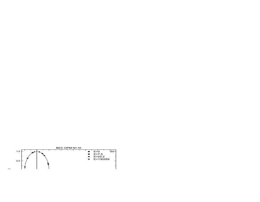
Figure 6: The eigenvalues $\lambda_{j},\;j=1,\ldots,2N$ (a) of the OPM (23) of the FPU Hamiltonian (4) with $N=10$ dof. (b) The eigenvalues of the OPM (2.2.1) of the BEC Hamiltonian (32) with the same number of dof $N$. (c) The eigenvalues of the IPM (2.2.1) of the BEC Hamiltonian (32) with $N=6$ dof.

4 Using SALI to Estimate the “Size” of Islands of Regular Motion

In this section, we estimate the “size” of islands of regular motion around stable SPOs using the Smaller Alignment Index (SALI) method Skokos, [2001]; Skokos et al., 2003a ; Skokos et al., 2003b ; Skokos et al., [2004], to distinguish between regular and chaotic orbits in the FPU and BEC Hamiltonians. The computation of the SALI has proved to be a very efficient method in revealing rapidly and with certainty the regular vs. chaotic nature of orbits, as it exhibits a completely different behavior for the two cases: It fluctuates around non–zero values for regular orbits, while it converges exponentially to zero for chaotic orbits. The behavior of the SALI for regular motion was studied and explained in detail by Skokos et al., 2003b , while a more analytical study of the behavior of the index in the case of chaotic motion can be found in Skokos et al., [2004].

As a first step, let us verify in the case of chaotic orbits of our $N$–degree of freedom systems, the validity of SALI’s dependence on the two largest Lyapunov exponents $L_{1}\equiv L_{\mathrm{max}}$ and $L_{2}$ proposed and numerically checked for $N=2$ and $3$, in Skokos et al., [2004]

$$\mathrm{SALI(t)}\propto e^{-(L_{1}-L_{2})t}.$$ (51)

This expression is very important as it implies that chaotic behavior can be decided by the exponential decay of this parameter, rather than the often questionable convergence of Lyapunov exponents to a positive value.

To check the validity of (51) let us take as an example the OHS mode (6) of the FPU Hamiltonian (4) using fixed boundary conditions, with $N=15$ dof and $\beta=1.04$, at the energy $E=21.6$ and calculate the Lyapunov exponents, as well as the corresponding SALI evolution. Plotting SALI as a function of time $t$ (in linear scale) together with its analytical formula (51) in Fig. 7(a), we see indeed an excellent agreement. Increasing further the energy to the value $E=26.6878$, it is in fact possible to verify expression (51), even in the case where the two largest Lyapunov exponents are nearly equal, as Fig. 7(b) evidently shows!

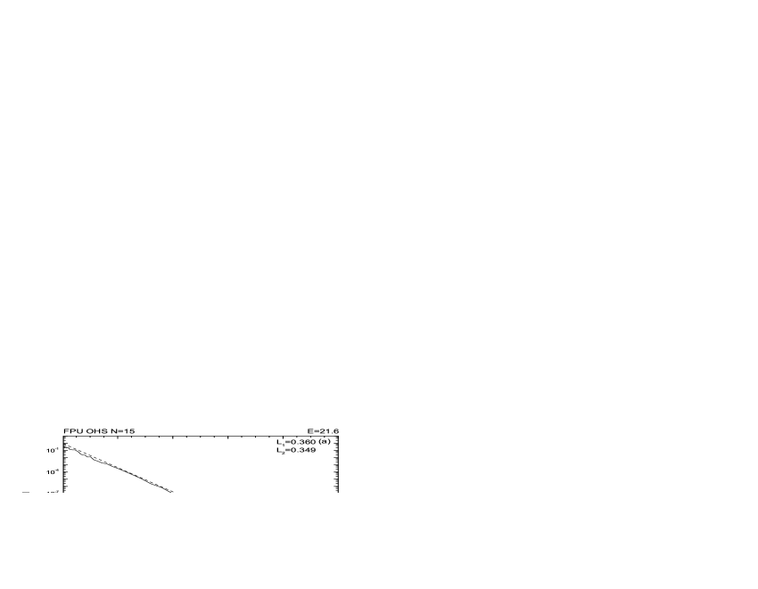
Figure 7: (a) The time evolution of the SALI (solid curve) and of the Eq. (51) (dashed line) at $E=21.6$ of the OHS mode (6) of the FPU Hamiltonian (4) with fixed boundary conditions. (b) Similar plot to panel (a) but for the larger energy $E=26.6878$ for which the two largest Lyapunov exponents $L_{1}$ and $L_{2}$ are almost equal while all the other positive ones are very close to zero. In both panels the agreement between the data (solid curve) and the derived function of Eq. (51) (dashed line) is remarkably good. Note that the horizontal axes in both panels are linear.

Exploiting now the different behavior of SALI for regular and chaotic orbits, we estimate approximately the “size” of regions of regular motion (or, “islands” of stability) in phase space, by computing SALI at points further and further away from a stable periodic orbit checking whether the orbits are still on a torus (SALI$\geq 10^{-8}$) or have entered a chaotic “sea” (SALI$<10^{-8}$) up to the integration time $t=4000$. The initial conditions are chosen perturbing all the positions of the stable SPO by the same quantity $dq$ and all the canonically conjugate momenta by the same $dp$ while keeping always constant the integral $F$, given by Eq. (33), in the case of the BEC Hamiltonian (32) and the energy $E$ in the case of the FPU Hamiltonian (4). In this way, we are able to estimate the approximate “magnitude” of the islands of stability for the OPM of Hamiltonian (4) and for the IPM and OPM of Hamiltonian (32) varying the energy $E$ and the number of dof $N$.

Figure 8: (a) “Size” of the islands of stability of the OPM (2.2.1) of the BEC Hamiltonian (32) for $N=4,\ 6$ and $8$ dof and SPOs constant energy $E=1$ before the first destabilization (see Table 3). (b) “Size” of the islands of stability of the same Hamiltonian and SPO as in (a) for $N=6$ dof and three different energies of the SPO before the first destabilization (see Table 3). (c) “Size” of the islands of stability of the same Hamiltonian as in (a) of the IPM (2.2.1) for $N=6$ dof and four different energies of the SPO. (d) “Size” of the islands of stability of the same Hamiltonian as in (a) of the IPM (2.2.1) for $\frac{E}{N}=\frac{10}{3}$. Here $E$ corresponds to the energy of the IPM.

In the case of the OPM solutions of both Hamiltonians, as the number of dof $N$ increases, for fixed energy $E$, the islands of stability eventually shrink to zero and the SPOs destabilize. For example, this is seen in Fig. 8(a) for the islands around the OPM (2.2.1) of the BEC Hamiltonian (32). A surprising behavior, however, is observed for the same SPO, if we keep $N$ fixed and increase the energy: Instead of diminishing, as expected from the FPU and other examples, the island of stability actually grows, as shown in Fig. 8(b), for the case of $N=6$ dof. In fact, it remains of considerable size until the SPO is destabilized for the first time, through period–doubling bifurcation at $E\approx 3.1875$, whereupon the island ceases to exist!

But what happens to the island of stability around the IPM solution of the BEC Hamiltonian (32), which does not become unstable for all values of $N$ and $E$ we studied? Does it shrink to zero at sufficiently large $E$ or $N$? From Fig. 8(c) we see that for a fixed value of $N$, the size of this island also increases as the energy increases. In fact, this SPO has large islands about it even if the energy is increased, keeping the ratio $E/N$ constant (see Fig. 8(d)). This was actually found to be true for considerably larger $E$ and $N$ values than shown in this figure.

5 Lyapunov Spectra and the Thermodynamic Limit

Finally, choosing again as initial conditions the unstable OPMs of both Hamiltonians, we determine some important statistical properties of the dynamics in the so–called thermodynamic limit of $E$ and $N$ growing indefinitely, while keeping $E/N$ constant. In particular, we compute the spectrum of the Lyapunov exponents of the FPU and BEC systems starting at the OPM solutions (23) and (2.2.1) for energies where these orbits are unstable. We thus find that the Lyapunov exponents are well approximated by smooth curves of the form $L_{i}\approx L_{1}e^{-\alpha i/N}$, for both systems, with $\alpha\approx 2.76$, $\alpha\approx 3.33$ respectively and $i=1,2,...,K(N)$ where $K(N)\approx 3N/4$ (see Fig. 9).

Figure 9: (a) Positive Lyapunov exponents spectrum of the OPM (23) of the FPU Hamiltonian (4) for fixed $\frac{E}{N}=\frac{3}{4}$. (b) Positive Lyapunov exponents spectrum of the OPM (2.2.1) of the BEC Hamiltonian (32) for fixed $\frac{E}{N}=\frac{3}{2}$. In both panels $i$ runs from $1$ to $N$.

Specifically, in the case of the OPM (23) of the FPU Hamiltonian (4) for fixed energy density $\frac{E}{N}=\frac{3}{4}$ we find

$$L_{i}(N)\approx L_{1}(N)e^{-2.76\frac{i}{N}},$$ (52)

while, in the case of the OPM (2.2.1) of the BEC Hamiltonian (32) for fixed energy density $\frac{E}{N}=\frac{3}{2}$, a similar behavior is observed,

$$L_{i}(N)\approx L_{1}(N)e^{-3.33\frac{i}{N}}.$$ (53)

These exponential formulas were found to hold quite well, up to $i=K(N)\approx 3N/4$. For the remaining exponents, the spectrum is seen to obey different decay laws, which are not easy to determine. As this appears to be a subtle matter, however, we prefer to postpone it for a future publication.

The functions (52) and (53), provide in fact, invariants of the dynamics, in the sense that, in the thermodynamic limit, we can use them to evaluate the average of the positive Lyapunov exponents (i.e. the Kolmogorov–Sinai entropy per particle) for each system and find that it is a constant characterized by the value of the maximum Lyapunov exponent $L_{1}$ and the exponent $\alpha$ appearing in them.

In Fig. 10 we compute the well–known Kolmogorov–Sinai entropy $h_{KS}(N)$ Pesin, [1976]; Hilborn, [1994] (solid curves), which is defined as the sum of the $N-1$ positive Lyapunov exponents,

$$h_{KS}(N)=\sum_{i=1}^{N-1}L_{i}(N),\ L_{i}(N)>0.$$ (54)

In this way, we find, for both Hamiltonians, that $h_{KS}(N)$ is an extensive thermodynamic quantity as it is clearly seen to grow linearly with $N$ ($h_{KS}(N)\propto N$), demonstrating that in their chaotic regions the FPU and BEC Hamiltonians behave as ergodic systems of statistical mechanics.

Finally, using Eqs. (52) and (53), as if they were valid for all $i=1,\ldots,N-1$, we approximate the sum of the positive Lyapunov exponents $L_{i}$, and calculate the $h_{KS}(N)$ entropy from Eq. (54) as

$$h_{KS}(N)\propto L_{\mathrm{max}}\frac{1}{-1+e^{\frac{2.76}{N}}},\,\,\,L_{\mathrm{max}}\approx 0.095,\mathrm{(FPU\ OPM)}$$ (55)

and

$$h_{KS}(N)\propto L_{\mathrm{max}}\frac{1}{-1+e^{\frac{3.33}{N}}},\,\,\,L_{\mathrm{max}}\approx 0.34,\mathrm{(BEC\ OPM)}.$$ (56)

In Fig. 10, we have plotted Eqs. (55) and (56) with dashed curves (adjusting the proportionality constants appropriately) and obtain nearly straight lines with the same slope as the data computed by the numerical evaluation of the $h_{KS}(N)$, from Eq. (54).

Figure 10: (a) The $h_{KS}(N)$ entropy of the OPM (23) of the FPU Hamiltonian (4) for fixed $\frac{E}{N}=\frac{3}{4}$ (solid curve) and the approximated formula (55) (dashed curve). (b) The $h_{KS}(N)$ entropy of the OPM (2.2.1) of the BEC Hamiltonian (32) for fixed $\frac{E}{N}=\frac{3}{2}$ (solid curve) and the approximated formula (56) (dashed curve).

6 Conclusions

In this paper we have investigated the connection between local and global dynamics of two $N$ dof Hamiltonian systems, describing $1$D nonlinear lattices with different origins known as the FPU and BEC systems. We focused on solutions located in the neighborhood of simple periodic orbits and showed that as the energy increases beyond the destabilization threshold, all positive Lyapunov exponents increase monotonically with two distinct power–law dependencies on the energy. We also computed the destabilization energy per particle of the OHS mode and of the two OPM orbits and found that it decays with a simple power–law of the form $E_{c}/N\propto N^{-\alpha}$, $\alpha=$ 1 or 2. One notable exception is the IPM orbit of the BEC Hamiltonian, which is found to be stable for any energy and number of dof we considered!

Furthermore, we found that as we increase the energy $E$ of both Hamiltonians for fixed $N$, the SPOs behave in very different ways: In the OPM case of the FPU Hamiltonian the eigenvalues of the monodromy matrix always move away from $-1$ with increasing energy, while in the OPM of the BEC Hamiltonian these eigenvalues return to $+1$, for very high energies. Nevertheless, this behavior does not represent a return of the system to a globally regular motion around the SPO as one might have thought. It simply reflects a local property of the SPO, as the orbits in its neighborhood still have positive Lyapunov exponents which are far from zero.

We have also been able to estimate the “size” of the islands of stability around the SPOs with the help of a recently introduced very efficient indicator called SALI and have seen them to shrink, as expected, when increasing $N$ for fixed $E$ in the case of the OPM of the FPU Hamiltonian. Of course, when we continue increasing the energy, keeping the number of dof fixed, the OPMs destabilize and the islands of stability are destroyed. Unexpectedly, however, in the case of the OPM of the BEC Hamiltonian these islands were seen to grow in size if we keep $N$ fixed and increase $E$ up to the destabilization threshold, a result that clearly requires further investigation. The peculiarity of our BEC Hamiltonian is even more vividly manifested in the fact that the islands of stability about its IPM orbit never vanish, remaining actually of significant size, even for very high values of $E$ and $N$ (keeping $E/N$ fixed).

Starting always near unstable SPOs, we also calculated the Lyapunov spectra characterizing chaotic dynamics in the regions of the OHS and OPM solutions of both Hamiltonians. Keeping $N$ fixed, we found energy values where these spectra were practically the same near SPOs which are far apart in phase space, indicating that the chaotic regions around these SPOs are visited ergodically by each other’s orbits. Finally, using an exponential law accurately describing these spectra, we were able to show, for both Hamiltonians, that the associated Kolmogorov–Sinai entropies per particle increase linearly with $N$ in the thermodynamic limit of $E\rightarrow\infty$ and $N\rightarrow\infty$ and fixed $E/N$ and, therefore, behave as extensive quantities of statistical mechanics.

Our results suggest, however, that, even in that limit, there may well exist Hamiltonian systems with significantly sized islands of stability around stable SPOs (like the IPM of the BEC Hamiltonian), which must be excluded from a rigorous statistical description. It is possible, of course, that these islands are too small in comparison with the extent of the chaotic domain on a constant energy surface and their “measure” may indeed go to zero in the thermodynamic limit. But as long as $E$ and $N$ are finite, they will still be there, precluding the global definition of probability densities, ensemble averages and the validity of the ergodic hypothesis over all phase space. Clearly, therefore, their study is of great interest and their properties worth pursuing in Hamiltonian systems of interest to physical applications.

7 Acknowledgements

This work was partially supported by the European Social Fund (ESF), Operational Program for Educational and Vocational Training II (EPEAEK II) and particularly the Program HERAKLEITOS, providing a Ph. D scholarship for one of us (C. A.). C. A. also acknowledges with gratitude the $3$ month hospitality, March–June $2005$, of the “Center for Nonlinear Phenomena and Complex Systems” of the University of Brussels. In particular, he thanks Professor G. Nicolis, Professor P. Gaspard and Dr. V. Basios for their instructive comments and useful remarks in many discussions explaining some fundamental concepts treated in this paper. The second author (T. B.) wishes to express his gratitude to the Max Planck Institute of the Physics of Complex Systems at Dresden, for its hospitality during his $3$ month visit March–June $2005$, when this work was completed. In particular, T. B. wants to thank Dr. Sergej Flach for numerous lively conversations and exciting arguments on the stability of multi–dimensional Hamiltonian systems. Useful discussions with Professors A. Politi, R. Livi, R. Dvorak, F. M. Izrailev and Dr. T. Kottos are also gratefully acknowledged. The third author (C. S.) was partially supported by the Research Committee of the Academy of Athens.

8 Figure Captions

1. The solid curve corresponds to the energy per particle $\frac{E_{c}}{N}$, for $\beta=1.04$, of the first destabilization of the OHS nonlinear mode (6) of the FPU system (4) obtained by the numerical evaluation of the Hill’s determinant in (19), while the dashed line corresponds to the function $\propto\frac{1}{N}$. Note that both axes are logarithmic.

2. The solid curve corresponds to the energy per particle $\frac{E_{c}}{N}$, for $\beta=1$, of the first destabilization of the nonlinear OPM (23) of the FPU system (4) obtained by the numerical evaluation of the Hill’s determinant, while the dashed line corresponds to the function $\propto\frac{1}{N^{2}}$. Note that both axes are logarithmic.

3. The solid curve corresponds to the energy per particle $\frac{E_{c}}{N}$ of the first destabilization of the OPM (2.2.1) of the BEC Hamiltonian (32) obtained by the numerical evaluation of the eigenvalues of the monodromy matrix of Eq. (2.2.2), while the dashed line corresponds to the function $\propto\frac{1}{N^{2}}$. Note that both axes are logarithmic.

4. The two distinct power–law behaviors in the evolution of the maximum Lyapunov exponent $L_{1}$ as the energy grows for the OPM (23) of the FPU Hamiltonian (4) for $N=10$. A similar picture is obtained for the $L_{2}$ and $L_{3}$ also, with similar exponents and the transition occurring at the same energy value (see text). Note that both axes are logarithmic.

5. (a) The spectrum of the positive Lyapunov exponents for fixed $N=10$ of the OPM (23) of the FPU Hamiltonian (4) as the energy grows. (b) Also for $N=10$, the OPM (2.2.1) of the BEC Hamiltonian (32) yields a similar picture as the energy is increased. (c) The Lyapunov spectrum of the OPM (23) of the FPU Hamiltonian (4) for $N=16$ and the OHS mode (6) of the same Hamiltonian and $N$, for periodic boundary conditions practically coincide at $E=6.82$ where both of them are destabilized. (d) The Lyapunov spectrum of the FPU OHS mode (6) with fixed boundary conditions for $N=15$ as the energy grows presents as shape which is qualitatively similar to what was found for the SPOs of panel (c).

6. The eigenvalues $\lambda_{j},\;j=1,\ldots,2N$ (a) of the OPM (23) of the FPU Hamiltonian (4) with $N=10$ dof. (b) The eigenvalues of the OPM (2.2.1) of the BEC Hamiltonian (32) with the same number of dof $N$. (c) The eigenvalues of the IPM (2.2.1) of the BEC Hamiltonian (32) with $N=6$ dof.

7. (a) The time evolution of the SALI (solid curve) and of the Eq. (51) (dashed line) at $E=21.6$ of the OHS mode (6) of the FPU Hamiltonian (4) with fixed boundary conditions. (b) Similar plot to panel (a) but for the larger energy $E=26.6878$ for which the two largest Lyapunov exponents $L_{1}$ and $L_{2}$ are almost equal while all the other positive ones are very close to zero. In both panels the agreement between the data (solid curve) and the derived function of Eq. (51) (dashed line) is remarkably good. Note that the horizontal axes in both panels are linear.

8. (a) “Size” of the islands of stability of the OPM (2.2.1) of the BEC Hamiltonian (32) for $N=4,\ 6$ and $8$ dof and SPOs constant energy $E=1$ before the first destabilization (see Table 3). (b) “Size” of the islands of stability of the same Hamiltonian and SPO as in (a) for $N=6$ dof and three different energies of the SPO before the first destabilization (see Table 3). (c) “Size” of the islands of stability of the same Hamiltonian as in (a) of the IPM (2.2.1) for $N=6$ dof and four different energies of the SPO. (d) “Size” of the islands of stability of the same Hamiltonian as in (a) of the IPM (2.2.1) for $\frac{E}{N}=\frac{10}{3}$. Here $E$ corresponds to the energy of the IPM.

9. (a) Positive Lyapunov exponents spectrum of the OPM (23) of the FPU Hamiltonian (4) for fixed $\frac{E}{N}=\frac{3}{4}$. (b) Positive Lyapunov exponents spectrum of the OPM (2.2.1) of the BEC Hamiltonian (32) for fixed $\frac{E}{N}=\frac{3}{2}$. In both panels $i$ runs from $1$ to $N$.

10. (a) The $h_{KS}(N)$ entropy of the OPM (23) of the FPU Hamiltonian (4) for fixed $\frac{E}{N}=\frac{3}{4}$ (solid curve) and the approximated formula (55) (dashed curve). (b) The $h_{KS}(N)$ entropy of the OPM (2.2.1) of the BEC Hamiltonian (32) for fixed $\frac{E}{N}=\frac{3}{2}$ (solid curve) and the approximated formula (56) (dashed curve).

References

- Abramowitz & Stegun, [1965] Abramowitz, M. and Stegun, I. [1965], “Handbook of Mathematical Functions”, (Dover, New York), Chap. 16.
- Aubry et al., [1996] Aubry, S., Flach, S., Kladko, K. and Oldbrich, E. [1996], “Manifestation of Classical Bifurcation in the Spectrum of the Integrable Quantum Dimer”, Phys. Rev. Lett., 76, (10), pp. 1607–1610.
- [3] Benettin, G., Galgani, L., Giorgilli, A. and Strelcyn, J. M. [1980], “Lyapunov Characteristic Exponents for Smooth Dynamical Systems and for Hamiltonian Systems; a Method for Computing all of Them, Part 1: Theory”, Meccanica, 15, March, pp. 9-20.
- [4] Benettin, G., Galgani, L., Giorgilli, A. and Strelcyn, J. M. [1980], “Lyapunov Characteristic Exponents for Smooth Dynamical Systems and for Hamiltonian Systems; a Method for Computing all of Them, Part 2: Numerical Applications”, Meccanica, 15, March, pp. 21-30.
- Benettin, [1984] Benettin, G. [1984], “Power–Law Behavior of Lyapunov Exponents in Some Conservative Dynamical Systems”Physica D, 13, pp. 211–220.
- Berman & Izrailev, [2004] Berman, G. P. and Izrailev, F. M. [2005], “The Fermi–Pasta–Ulam Problem: 50 Years of Progress”, Chaos 15 015104.
- Bountis ed., [1992] Bountis, T. ed. [1992], “Proton Transfer in Hydrogen–Bonded Systems”, Proceedings of NATO ARW, Plenum, London.
- Budinsky & Bountis, [1983] Budinsky, N. and Bountis, T. [1983], “Stability of Nonlinear Modes and Chaotic Properties of D Fermi–Pasta–Ulam Lattices”, Physica D, 8, pp. 445 – 452.
- Cafarella et al., [2004] Cafarella, A., Leo, M. and Leo, R. A. [2003], “Numerical Analysis of the One–Mode Solutions in the Fermi–Pasta–Ulam System”, Phys. Rev. E, 69, pp. 046604.
- Chirikov, [1979] Chirikov, B. V. [1979], “A Universal Instability of Many–Dimensional Oscillator Systems”, Phys. Rep., 52, (5), pp. 263–379.
- Contopoulos, [2002] Contopoulos, G. [2002], Order and Chaos in Dynamical Astronomy, (Springer), Astronomy and Astrophysics Library.
- Copson, [1935] Copson, E. T. [1935], An Introduction to the Theory of Functions of a Complex Variable, (Oxford Univ. Press, Oxford), Chap. 14.
- Dalfovo et al., [1999] Dalfovo, F., Giorgini, S., Pitaevskii, L. P. and Stringari, S. [1999], “Theory of Bose-Einstein Condensation in Trapped Gases”, Rev. Mod. Phys., 71, pp. 463-512.
- De Luca et al., [1995] De Luca, J., Lichtenberg, A. J. and Lieberman, M. A. [1995], “Time Scale to Ergodicity in the Fermi–Pasta–Ulam System”, Chaos, 5, (1), pp. 283–297.
- De Luca & Lichtenberg, [2002] De Luca, J. and Lichtenberg, A. J. [2002], “Transitions and Time Scales to Equipartition in Oscillator Chains: Low Frequency Initial Conditions”, Phys. Rev. E, 66, (2), pp. 026206.
- Eisenberg et al., [1998] Eisenberg, H. S., Silberberg, Y., Morandotti, R., Boyd, A. R. & Aitchison, J. S. [1998], “Discrete Spatial Optical Solitons in Waveguide Arrays”, Phys. Rev. Lett. 81(16), pp. 3383–3386.
- Fermi et al., [1955] Fermi, E., Pasta, J. and Ulam, S. [1955], “Studies of Nonlinear Problems”, Los Alamos document LA–1940. See also: “Nonlinear Wave Motion”, [1974], Am. Math. Soc. Providence, 15, Lectures in Appl. Math., ed. Newell A. C.
- Flach & Willis, [1998] Flach, S. and Willis, C. R. [1998], “Discrete Breathers”, Phys. Rep., 295, (5), pp. 181–264.
- Flach et al., [2005] Flach, S., Ivanchenko, M. V. and Kanakov, O. I. [2005], “q-Breathers and the Fermi–Pasta–Ulam Problem”, Phys. Rev. Let., 95, pp. 064102-1–064102-4.
- Fleischer et al., [2003] Fleischer, J. W., Segev, M., Efremidis, N. K. & Christodoulides, D. N. [2003], “Observation of Two–Dimensional Discrete Solitons in Optically Induced Nonlinear Photonic Lattices”, Nature 422(6928), pp. 147–150.
- Ford, [1992] Ford, J. [1992], “The Fermi–Pasta–Ulam Problem: Paradox Turned Discovery”, Physics Reports, 213, pp. 271–310.
- Hilborn, [1994] Hilborn, R. C. [1994], Chaos and Nonlinear Dynamics, (Oxford University Press).
- Izrailev & Chirikov, [1966] Izrailev, F. M. and Chirikov, B. V. [1966], “Statistical Properties of a Nonlinear String”, Sov. Phys. Dok., 11, pp. 30.
- Ketterle et al., [1999] Ketterle, W., Durfee, D. S. and Stamper–Kurn, D. M. [1999], “Bose–Einstein Condensation in Atomic Gases”, in International School of Physics, eds. Fermi, E., Course , edited by Inguscio, M., Stringari, S. and Wieman, C., (IOS Press, Amsterdam).
- Lichtenberg & Lieberman, [1991] Lichtenberg, A. J. and Lieberman, M. A [1991], “Regular and Stochastic Motion”, 2nd edition (Springer Verlag, New York).
- Livi et al., [1986] Livi, R., Politi, A. and Ruffo, S., [1986], “Distribution of Characteristic Exponents in the Thermodynamic Limit”, J. Phys. A: Math. Gen., 19, pp. 2033–2040.
- MacKay & Meiss, [1987] MacKay, R. S. and Meiss, J. D. [1987], “Hamiltonian Dynamical Systems”, (Adam Hilger, Bristol).
- Magnus & Winkler, [1966] Magnus, W. and Winkler, S. [1966], “Hill’s Equation”, (Interscience, New York).
- Ooyama et al., [1969] Ooyama, N., Hirooka, H. and Saitô, N. [1969], “Computer Studies on the Approach to Thermal Equilibrium in Coupled Anharmonic Oscillators. II. One Dimensional Case”, J. Phys. Soc. of Japan, 27, (4), pp. 815 – 824.
- Pesin, [1976] Pesin, Ya. B. [1976], “Lyapunov Characteristic Indexes and Ergodic Properties of Smooth Dynamic Systems with Invariant Measure”, Dokl. Acad. Nauk. SSSR, 226, (4), pp. 774–777.
- Poggi & Ruffo, [1997] Poggi, P. & Ruffo, S. [1997], “Exact Solutions in the FPU Oscillator Chain”, Physica D, 103, pp. 251–272.
- Prosmiti & Farantos, [1995] Prosmiti, R. & Farantos, S. C. [1995], “Periodic Orbits, Bifurcation Diagrams and the Spectroscopy of System”, J. Chem. Phys., 1039, pp. 3299 – 3314.
- Rechester et al., [1979] Rechester, A. B., Rosenbluth, M. N. & White, R. B. [1979], “Calculation of the Kolmogorov Entropy for Motion Along a Stochastic Magnetic Field”, Phys. Rev. Lett., 42, pp. 1247.
- Scandale & Turchetti, eds. [1991] Scandale, W. & Turchetti, G., eds. [1991], “Nonlinear Problems in Future Particle Accelerators”, (World Scientific, Singapore).
- Sato et al., [2003] Sato, M. Hubbard, B. E., Sievers, A. J., Ilic, B., Czaplewski, D. A. & Craighead, H. G. [2003], “Observation of Locked Intrinsic Localized Vibrational Modes in a Micromechanical Oscillator Array” Phys. Rev. Lett., 90(4), pp. 044102.
- Schwarz, [1999] Schwarz, U. T., English, L. Q., & Sievers A. J. [1999], “Experimental Generation and Observation of Intrinsic Localized Spin Wave Modes in an Antiferromagnet”, Phys. Rev. Lett., 83(1), pp. 223–226.
- Simó ed., [1999] Simó, C. ed. [1999], Hamiltonian Systems with Three or More Degrees of Freedom, (Kluwer Academic Publishers), 533, NATO ASI.
- Skokos, [2001] Skokos, Ch. [2001], “Alignment Indices: A New, Simple Method for Determining the Ordered or Chaotic Nature of Orbits”, J. Phys. A, 34, pp. 10029 – 10043.
- [39] Skokos, Ch., Antonopoulos, Ch., Bountis, T. C. and Vrahatis, M. N. [2003], “Smaller Alignment Index (SALI): Determining the Ordered or Chaotic Nature of Orbits in Conservative Dynamical Systems”, in Proceedings of the Conference Libration Point Orbits and Applications, eds. Gomez, G., Lo, M. W. and Masdemont, J. J., (World Scientific), pp. 653 – 664.
- [40] Skokos, Ch., Antonopoulos, Ch., Bountis, T. C. and Vrahatis, M. N. [2003], “How does the Smaller Alignment Index (SALI) Distinguish Order from Chaos?”, Prog. Theor. Phys. Supp., 150, pp. 439 – 443
- Skokos et al., [2004] Skokos, Ch., Antonopoulos, Ch., Bountis, T. C. and Vrahatis, M. N. [2004], “Detecting Order and Chaos in Hamiltonian Systems by the SALI Method”, J. Phys. A, 37, pp. 6269 – 6284.
- Smerzi & Trombettoni, [2003] Smerzi, A. and Trombettoni, A. [2003], “Nonlinear Tight–Binding Approximation for Bose–Einstein Condensates in a Lattice”, Phys. Rev., A68, 023613.
- Trombettoni & Smerzi, [2001] Trombettoni, A. and Smerzi, A. [2001], “Discrete Solitons and Breathers with Dilute Bose–Einstein Condensates”, Phys. Rev. Lett., 86, pp. 2353.
- Wiggins, [1988] Wiggins, S. [1988], “Global Bifurcations and Chaos : Analytical Methods”, (New York, Springer Verlag).