Multiple permanent-wave trains in nonlinear systems

Abstract

Multiple permanent-wave trains in nonlinear systems are constructed by the asymptotic tail-matching method. Under some general assumptions, simple criteria for the construction are presented. Applications to fourth-order systems and coupled nonlinear Schrödinger equations are discussed.

1 Introduction

Nonlinear wave systems have been studied for a few decades. Much progress has been made on integrable equations where the inverse scattering transform method can be applied [1]. For non-integrable equations, the general analytical treatment has been elusive so far and will likely remain so in the near future. A less ambitious goal, then, would be to generally study the permanent waves in non-integrable systems. Such waves often contain valuable information on the system’s general solution behaviors. An interesting fact is that, in many non-integrable systems, simple permanent waves can be matched together and form multiple permanent-wave trains ([2], [3], [4], [5], [6], [7], etc.). If solitary waves exist, multiple solitary-wave trains can be constructed by a perturbation method proposed by Karpman and Solov’ev [8] and Gorshkov and Ostrovsky [9] (see [3]). If permanent waves with exponentially decaying and oscillating tails are present, the existence of countably infinite multiple permanent-wave trains has been proved for certain types of nonlinear systems by variational methods ([4], [5]). In this paper, if a nonlinear wave system allows permanent waves which exponentially approach a constant at infinity, we will construct widely-separated multiple permanent-wave trains by a new and general method, namely, the asymptotic tail-matching method. This method is stimulated in part by another matching method for non-local solitary waves (see [6] and [7]). Under some general assumptions, we will show that an arbitrary number of permanent waves can be matched together and form multiple permanent-wave trains if and only if the exponential tails of these permanent waves satisfy certain simple algebraic conditions. These conditions will also determine the spacings between adjacent permanent waves if such matching takes place. This asymptotic tail-matching method differs from Karpman et al’s perturbation method in two major aspects. First, it can be applied directly to the matching of kink and anti-kink type permanent waves. Second, its results are explicit, simple and insightful. As applications of these general results, we will discuss fourth-order systems and the coupled nonlinear Schrödinger equations. For fourth-order systems which allow permanent waves exponentially and oscillatorily approaching a constant at infinity, we will show that countably infinite multiple permanent-wave trains exist and can be readily constructed. Thus the results in [4] and [5] are reproduced. For the coupled nonlinear Schrödinger equations, we will show that countably infinite multiple solitary-wave trains can be constructed in a large portion of the parameter space. Numerical results will also be presented and compared with the theoretical predictions when appropriate.

2 Construction of multiple permanent-wave trains

We consider a general nonlinear wave system

$$F(U,D_{x},D_{t})=0,$$ (2.1)

where $U$ is the unknown vector variable, and $F$ is a nonlinear vector function. Suppose it allows permanent waves of certain form which, when substituted into Eq. (2.1), reduces it into an autonomous complex system of first-order nonlinear ordinary differential equations

$$d\Phi/dx=G(\Phi),$$ (2.2)

where $\Phi(x)$ is a $n$-component vector variable. If Eq. (2.2) has permanent wave solutions which exponentially approach a constant at infinity, then we next will develop a new method to determine if those permanent waves can be matched together and form widely-separated multiple permanent-wave trains or not. The idea is to perturb each permanent wave such that the exponential tails of each perturbed wave match those of the adjacent permanent waves. We first discuss the matching of solitary waves, followed by that of general permanent waves.

2.1 Solitary-wave trains

Suppose Eq. (2.2) allows solitary waves $\Phi(x)$ which exponentially decay to zero as $|x|\rightarrow\infty$. We make the following general assumptions:

1. the eigenvalues of the constant (Jacobian) matrix $\nabla G(0)$ all have non-zero real parts;

2. for any solitary wave $\Phi(x)$, the linear behavior dominates at infinity, i.e., as $x\rightarrow\infty$ or $-\infty$, $\Phi(x)$ approaches a solution of the linear equation

   $$d\tilde{\Phi}/dx=\nabla G(0)\tilde{\Phi};$$ (2.3)

3. for any solitary wave $\Phi(x)$, the linearized equation of (2.2) around $\Phi(x)$

   $$d\tilde{\Phi}/dx=\nabla G(\Phi)\tilde{\Phi}$$ (2.4)

   and its adjoint equation

   $$-d\Psi/dx=\nabla G^{*\mbox{\tiny\it T}}(\Phi)\Psi$$ (2.5)

   each have a single linearly independent localized solution. Here “T” represents the transpose and “*” the complex conjugate.

Remark: Since Eq. (2.2) is autonomous, any spatial translation of $\Phi(x)$ is still (2.2)’s solution. Therefore Eq. (2.4) always has a nontrivial localized solution $d\Phi(x)/dx$. The requirement for Eq. (2.4) is just that $d\Phi(x)/dx$ is its single linearly independent localized solution. This can be guaranteed if $\Phi(x)$ is isolated in $H^{1}(R,R^{2})$ up to spatial translations (the so-called non-degenerency condition in some of the literature. See [4]).

We also introduce the following notations. In view of assumption A1, let us denote $\nabla G(0)$’s eigenvalues as $\lambda_{1},\lambda_{2},\dots,\lambda_{n}$ where

$$\mbox{Re}(\lambda_{1})\leq\mbox{Re}(\lambda_{2})\leq\dots\leq\mbox{Re}(\lambda_{s})<0<\mbox{Re}(\lambda_{s+1})\leq\mbox{Re}(\lambda_{s+2})\leq\dots\leq\mbox{Re}(\lambda_{n}).$$ (2.6)

Suppose for an eigenvalue $\lambda$, $\nabla G(0)$ has a chain of eigenvector and generalized eigenvectors $v_{i}\;(i=1,\dots,l)$ such that

$$(\nabla G(0)-\lambda I)v_{1}=0,$$ (2.7)

$$(\nabla G(0)-\lambda I)v_{i+1}=v_{i},\hskip 17.07182pti=1,\dots,l-1.$$ (2.8)

Define the polynomial functions $\xi_{i}(x)\;(i=1,\dots,l)$ as

$$\xi_{i}(x)=v_{i}+xv_{i-1}+\dots+\frac{x^{i-1}}{(i-1)!}v_{1},\hskip 28.45274pti=1,\dots,l,$$ (2.9)

then

$$\xi^{\prime}_{i+1}(x)=\xi_{i}(x),$$ (2.10)

and $\{\xi_{i}(x)e^{\lambda x},\;i=1,\dots,l\}$ form a chain of linearly independent solutions of Eq. (2.3). According to the theory of linear differential equations with constant coefficients, we can find such chains of solutions which together form a fundamental set of solutions of Eq. (2.3). Thus according to assumption A2, we have

$$\Phi(x)\longrightarrow\left\{\begin{array}[]{l}\sum_{i=1}^{s}c_{i}\xi_{i}(x)e^{\lambda_{i}x},\hskip 22.76228ptx\rightarrow\infty,\\ \sum_{i=s+1}^{n}c_{i}\xi_{i}(x)e^{\lambda_{i}x},\hskip 11.38092ptx\rightarrow-\infty,\end{array}\right.$$ (2.11)

where $c_{i}\;(i=1,\dots,n)$ are complex constants. We point out that in the special case where $\nabla G(0)$ has $n$ linearly independent eigenvectors, $\{\xi_{i},\>i=1,\dots,n\}$ are just those constant eigenvectors. The fundamental matrix of the adjoint equation (2.5) at infinity is

$$[\eta_{1}e^{-\lambda_{1}^{*}x}\;\;\eta_{2}e^{-\lambda_{2}^{*}x}\;\;\dots\;\;\eta_{n}e^{-\lambda_{n}^{*}x}],$$ (2.12)

where

$$[\eta_{1}\;\>\eta_{2}\;\>\dots\;\>\eta_{n}]=\{[\xi_{1}\;\>\xi_{2}\;\>\dots\;\>\xi_{n}]^{-1}\}^{*\mbox{\tiny\it T}}.$$ (2.13)

Note that for $1\leq i,j\leq n$,

$$\xi_{i}(x)\cdot\eta^{*}_{j}(x)=\left\{\begin{array}[]{l}1,\hskip 14.22636pti=j,\\ 0,\hskip 14.22636pti\neq j.\end{array}\right.$$ (2.14)

Thus for the single linearly independent localized solution $\Psi(x)$ of Eq. (2.5), we have

$$\Psi(x)\longrightarrow\left\{\begin{array}[]{l}\sum^{s}_{i=1}d_{i}\eta_{i}(x)e^{-\lambda^{*}_{i}x},\hskip 42.67912ptx\rightarrow-\infty,\\ \sum^{n}_{i=s+1}d_{i}\eta_{i}(x)e^{-\lambda^{*}_{i}x},\hskip 31.2982ptx\rightarrow\infty,\end{array}\right.$$ (2.15)

where $d_{i}\;(i=1,\dots,n)$ are complex constants.

Now suppose $\{\Phi^{(1)},\Phi^{(2)},\dots,\Phi^{(N)}\}$ are $N$ solitary waves of Eq. (2.2) with

$$\Phi^{(k)}(x)\longrightarrow\left\{\begin{array}[]{l}\sum_{i=1}^{s}c_{i}^{(k)}\xi_{i}(x)e^{\lambda_{i}x},\hskip 19.91684ptx\rightarrow\infty,\\ \sum_{i=s+1}^{n}c_{i}^{(k)}\xi_{i}(x)e^{\lambda_{i}x},\hskip 8.5359ptx\rightarrow-\infty.\end{array}\right.$$ (2.16)

For each $\Phi^{(k)}$, the single linearly independent localized solution $\Psi^{(k)}$ of the adjoint equation

$$-d\Psi^{(k)}/dx=\nabla G^{*\mbox{\tiny\it T}}(\Phi^{(k)})\Psi^{(k)}$$ (2.17)

has the following asymptotic behavior at infinity:

$$\Psi^{(k)}(x)\longrightarrow\left\{\begin{array}[]{l}\sum^{s}_{i=1}d^{(k)}_{i}\eta_{i}(x)e^{-\lambda^{*}_{i}x},\hskip 39.83368ptx\rightarrow-\infty,\\ \sum^{n}_{i=s+1}d^{(k)}_{i}\eta_{i}(x)e^{-\lambda^{*}_{i}x},\hskip 28.45274ptx\rightarrow\infty.\end{array}\right.$$ (2.18)

Consider a new solitary wave which looks like a superposition of the above $N$ solitary waves $\{\Phi^{(k)}\}$ widely separated, with the $k$-th wave $\Phi^{(k)}$ located at $x=x_{k}$ $(k=1,2,\dots,N)$. Let

$$x_{1}<x_{2}<\dots<x_{N},$$ (2.19)

and denote

$$\triangle_{k}=x_{k+1}-x_{k}\;(\gg 1),\hskip 8.5359ptk=1,2,\dots,N-1.$$ (2.20)

We will call this new solitary wave as a $N$-pulse wavetrain. It can be constructed explicitly by the following theorem.

Theorem 1

Under the assumptions A1, A2, A3 and the above notations, the $N$ solitary waves $\{\Phi^{(1)},\dots,\Phi^{(N)}\}$ can match each other and form a widely-separated $N$-pulse wavetrain if and only if the spacings $\triangle_{k}\;(\gg 1)\;(k=1,\dots,N-1)$ asymptotically satisfy the following $N$ conditions

$$\sum^{n}_{j=s+1}c_{j}^{(2)}d_{j}^{(1)*}e^{-\lambda_{j}\triangle_{1}}=0,$$ (2.21a)

$$\sum^{s}_{j=1}c_{j}^{(k-1)}d_{j}^{(k)*}e^{\lambda_{j}\triangle_{k-1}}=\sum^{n}_{j=s+1}c_{j}^{(k+1)}d_{j}^{(k)*}e^{-\lambda_{j}\triangle_{k}},\hskip 14.22636pt(2\leq k\leq N-1),$$ (2.21b)

$$\sum^{s}_{j=1}c_{j}^{(N-1)}d_{j}^{(N)*}e^{\lambda_{j}\triangle_{N-1}}=0.$$ (2.21c)

The relative errors in Eqs. (1) are exponentially small with the spacings.

We will prove this theorem by the asymptotic tail-matching method to be developed next.

Proof: Suppose such a $N$-pulse wavetrain $\Phi(x)$ exists. Then around the $k$-th wave $(2\leq k\leq N-1)$, the solution is

$$\Phi(x)=\Phi^{(k)}(x-x_{k})+\tilde{\Phi}^{(k)}(x-x_{k}),$$ (2.22)

where $\tilde{\Phi}^{(k)}\ll 1$. The linearized equation for $\tilde{\Phi}^{(k)}$ is

$$d\tilde{\Phi}^{(k)}(x)/dx=\nabla G(\Phi^{(k)}(x))\;\tilde{\Phi}^{(k)}(x).$$ (2.23)

According to assumption A3, Eq. (2.23) has a single linearly independent localized solution which is $d\Phi^{(k)}(x)/dx$. From Eq. (2.16) we get

$$d\Phi^{(k)}(x)/dx\longrightarrow\sum^{s}_{i=1}c_{i}^{(k)}(\xi^{\prime}_{i}(x)+\lambda_{i}\xi_{i}(x))\;e^{\lambda_{i}x},\hskip 14.22636ptx\rightarrow\infty.$$ (2.24)

Clearly not all the $c_{i}^{(k)}$’s $(i=1,\dots,s)$ are equal to zero. Without loss of generality, we assume that $c_{1}^{(k)}\neq 0$. Then we denote the other $n-1$ solutions of Eq. (2.23) as $\tilde{\Phi}_{j}^{(k)}\;(j=2,\dots,n)$. We require that

$$\tilde{\Phi}_{j}^{(k)}(x)\longrightarrow\xi_{j}(x)e^{\lambda_{j}x},\hskip 14.22636ptx\rightarrow\infty.$$ (2.25)

As $x\rightarrow-\infty$, we generally have

$$\tilde{\Phi}_{j}^{(k)}(x)\longrightarrow\sum^{n}_{i=1}a_{ji}^{(k)}\xi_{i}(x)e^{\lambda_{i}x},\hskip 11.38092ptj=2,\dots,n,$$ (2.26)

where $a_{ji}^{(k)}$ are constants. Since $c_{1}^{(k)}\neq 0$, these $n$ solutions $\{d\Phi^{(k)}/dx,\tilde{\Phi}_{2}^{(k)},\dots,\tilde{\Phi}_{n}^{(k)}\}$ are linearly independent at $x$ equal to infinity, and they form a fundamental set of solutions of Eq. (2.23). Thus the general solution for $\tilde{\Phi}^{(k)}(x-x_{k})$ is

$$\tilde{\Phi}^{(k)}(x-x_{k})=h_{1}\frac{d\Phi^{(k)}}{dx}(x-x_{k})+\sum^{n}_{j=2}h_{j}\tilde{\Phi}_{j}^{(k)}(x-x_{k}),$$ (2.27)

where $h_{j}\;(j=1,\dots,n)$ are constants. The first term in (2.27) can be absorbed into $\Phi^{(k)}(x-x_{k})$ and cause a position shift to it. By normalization we make $h_{1}=0$. When $x_{k}\ll x\ll x_{k+1}$, dropping the exponentially small terms, we get

$$\tilde{\Phi}^{(k)}(x-x_{k})\longrightarrow\sum^{n}_{j=s+1}h_{j}\xi_{j}(x-x_{k})e^{\lambda_{j}(x-x_{k})}.$$ (2.28)

Similarly, when $x_{k-1}\ll x\ll x_{k}$, we have

$$\tilde{\Phi}^{(k)}(x-x_{k})\longrightarrow\sum_{j=1}^{s}(\sum_{i=2}^{n}a_{ij}^{(k)}h_{i})\xi_{j}(x-x_{k})e^{\lambda_{j}(x-x_{k})}.$$ (2.29)

The key idea in the asymptotic tail-matching method is that, in order for the matching to occur, we need to require that in the region $x_{k}\ll x\ll x_{k+1}$, $\tilde{\Phi}^{(k)}(x-x_{k})$’s exponentially growing terms match the left tail of the right-hand wave $\Phi^{(k+1)}(x-x_{k+1})$; in the region $x_{k-1}\ll x\ll x_{k}$, $\tilde{\Phi}^{(k)}(x-x_{k})$’s exponentially decaying terms match the right tail of the left-hand wave $\Phi^{(k-1)}(x-x_{k-1})$. In the region $x_{k}\ll x\ll x_{k+1}$, this requirement is

$$\sum_{j=s+1}^{n}h_{j}\xi_{j}(x-x_{k})e^{\lambda_{j}(x-x_{k})}=\sum_{j=s+1}^{n}c_{j}^{(k+1)}\xi_{j}(x-x_{k+1})e^{\lambda_{j}(x-x_{k+1})};$$ (2.30)

and in the region $x_{k-1}\ll x\ll x_{k}$, it is

$$\sum_{j=1}^{s}(\sum_{i=2}^{n}a_{ij}^{(k)}h_{i})\xi_{j}(x-x_{k})e^{\lambda_{j}(x-x_{k})}=\sum_{j=1}^{s}c_{j}^{(k-1)}\xi_{j}(x-x_{k-1})e^{\lambda_{j}(x-x_{k-1})}.$$ (2.31)

We now need to select the constants $h_{j}\;(j=2,\dots,n)$ and spacings $\triangle_{k}\;(k=1,\dots,N-1)$ so that the above two conditions are satisfied.

First consider condition (2.30). Recall that functions $\{\xi_{j}(x)\}$ are of the form (2.9). If for $\lambda=\lambda_{m}\;(s+1\leq m\leq n)$, the chain of such functions is $\{\xi_{m},\dots,\xi_{m+l-1}\}$, where $\xi_{m}$ is a constant vector and

$$\xi^{\prime}_{j+1}(x)=\xi_{j}(x),\hskip 14.22636ptj=m,\dots,m+l-2.$$ (2.32)

Then we select $\{h_{m},\dots,h_{m+j-1}\}$ from the equation

$$\sum_{j=m}^{m+l-1}h_{j}\xi_{j}(x-x_{k})e^{\lambda(x-x_{k})}=\sum_{j=m}^{m+l-1}c_{j}^{(k+1)}\xi_{j}(x-x_{k+1})e^{\lambda(x-x_{k+1})}.$$ (2.33)

The right hand side of this equation is

$$\sum_{j=m}^{m+l-1}c_{j}^{(k+1)}\xi_{j}(x-x_{k}-\triangle_{k})e^{\lambda(x-x_{k})}e^{-\lambda\triangle_{k}}$$

$$=\sum_{j=m}^{m+l-1}c_{j}^{(k+1)}(\sum_{i=0}^{j-m}\frac{(-\triangle_{k})^{i}}{i!}\frac{d^{i}\xi_{j}}{dx^{i}}(x-x_{k}))e^{\lambda(x-x_{k})}e^{-\lambda\triangle_{k}}$$

$$=\sum_{j=m}^{m+l-1}\sum_{i=m}^{j}c_{j}^{(k+1)}\frac{(-\triangle_{k})^{j-i}}{(j-i)!}\xi_{i}(x-x_{k})e^{\lambda(x-x_{k})}e^{-\lambda\triangle_{k}}$$

$$=\sum_{i=m}^{m+l-1}(\sum_{j=i}^{m+l-1}\frac{(-\triangle_{k})^{j-i}}{(j-i)!}c_{j}^{(k+1)})e^{-\lambda\triangle_{k}}\xi_{i}(x-x_{k})e^{\lambda(x-x_{k})}.$$ (2.34)

Now we choose $h_{i}\;(i=m,\dots,m+l-1)$ to be

$$h_{i}=(\sum_{j=i}^{m+l-1}\frac{(-\triangle_{k})^{j-i}}{(j-i)!}c_{j}^{(k+1)})e^{-\lambda\triangle_{k}},\hskip 14.22636pti=m,\dots,m+l-1,$$ (2.35)

then Eq. (2.33) is valid. Repeating this procedure for the other chains of {$\xi_{j}(x)$} functions in the form (2.9), we can successfully select $h_{i}\;(i=s+1,\dots,n)$ so that condition (2.30) is satisfied.

Next consider condition (2.31). Similar analysis shows that we can reduce its right hand side to

$$\sum^{s}_{j=1}c_{j}^{(k-1)}\xi_{j}(x-x_{k-1})e^{\lambda_{j}(x-x_{k-1})}=\sum^{s}_{j=1}\alpha_{j}e^{\lambda_{j}\triangle_{k-1}}\xi_{j}(x-x_{k})e^{\lambda_{j}(x-x_{k})},$$ (2.36)

where $\alpha_{j}\;(j=1,\dots,s)$ are constants and determined by $c_{j}^{(k-1)}\;(j=1,\dots,s)$ and $\triangle_{k-1}$. Then condition (2.31) becomes

$$\sum^{s}_{i=2}a^{(k)}_{ij}h_{i}=\alpha_{j}e^{\lambda_{j}\triangle_{k-1}}-\sum^{n}_{i=s+1}a^{(k)}_{ij}h_{i},\hskip 14.22636ptj=1,\dots,s.$$ (2.37)

This is a linear system of $s$ equations for $s-1$ unknowns $h_{i}\;(i=2,\dots,s)$. We now show that the matrix $(a_{ij}^{(k)})_{s\times(s-1)}$ on the left side of Eq. (2.37) has rank $s-1$. Consider the solution of Eq. (2.23)

$$T(x)=\sum_{j=2}^{s}p_{j}\tilde{\Phi}_{j}^{(k)}(x),$$ (2.38)

where $p_{j}\;(j=2,\dots,s)$ are constants. Dropping exponentially small terms we get

$$T(x)\longrightarrow\left\{\begin{array}[]{l}0,\hskip 28.45274ptx\rightarrow\infty,\\ \sum_{j=1}^{s}(\sum^{s}_{i=2}a_{ij}^{(k)}p_{i})\xi_{j}(x)e^{\lambda_{j}x},\hskip 8.5359ptx\rightarrow-\infty.\end{array}\right.$$ (2.39)

According to assumption A3, the only localized solution of Eq. (2.23) is $d\Phi^{(k)}(x)/dx$. Moreover, $c_{1}^{(k)}$ in (2.24) is non-zero. Thus $T(x)$ can not be a localized solution. In other words, the linear system of equations

$$\sum^{s}_{i=2}a_{ij}^{(k)}p_{i}=0,\hskip 28.45274ptj=1,\dots,s,$$ (2.40)

has no non-trivial solutions for $p_{i}\;(i=1,\dots,s)$. Therefore the matrix $(a_{ij}^{(k)})_{s\times(s-1)}$ has rank $s-1$. Without loss of generality, we assume that the last $(s-1)$ rows of the matrix are linearly independent. Then the linear system

$$\sum^{s}_{i=2}a_{ij}^{(k)}h_{i}=\alpha_{j}e^{\lambda_{j}\triangle_{k-1}}-\sum^{n}_{i=s+1}a^{(k)}_{ij}h_{i},\hskip 28.45274ptj=2,\dots,s,$$ (2.41)

has a unique solution for $h_{i}\;(i=2,\dots,s)$. With $h_{i}\;(i=2,\dots,n)$ given by (2.35) and (2.41), the only matching condition left to be satisfied now is

$$\sum^{s}_{i=2}a_{i1}^{(k)}h_{i}=\alpha_{1}e^{\lambda_{1}\triangle_{k-1}}-\sum^{n}_{i=s+1}a^{(k)}_{i1}h_{i},$$ (2.42)

which will determine the spacings of this $N$-pulse wavetrain. Since the matrix $(a_{ij}^{(k)})_{s\times(n-1)}$ is not readily available, to determine the spacings from Eq. (2.42) is difficult. But this can be easily done with the aid of the solution $\Psi^{(k)}$ of the adjoint equation (2.17). With $h_{i}\;(i=2,\dots,n)$ given by (2.35) and (2.41), it is easy to show that Eqs. (2.28) and (2.29) become

$$\tilde{\Phi}^{(k)}(x-x_{k})\longrightarrow\sum_{j=s+1}^{n}c_{j}^{(k+1)}\xi_{j}(x-x_{k+1})e^{\lambda_{j}(x-x_{k+1})},\hskip 28.45274ptx_{k}\ll x\ll x_{k+1},$$ (2.43)

and

$$\tilde{\Phi}^{(k)}(x-x_{k})\longrightarrow w\;\xi_{1}(x-x_{k-1})e^{\lambda_{1}(x-x_{k-1})}+\sum_{j=2}^{s}c_{j}^{(k-1)}\xi_{j}(x-x_{k-1})e^{\lambda_{j}(x-x_{k-1})},\hskip 22.76228ptx_{k-1}\ll x\ll x_{k},$$ (2.44)

where $w$ is a constant. Condition (2.42) is equivalent to

$$w=c_{1}^{(k-1)}.$$ (2.45)

For $x_{k-1}\ll y_{1}\ll x_{k}$ and $x_{k}\ll y_{2}\ll x_{k+1}$, we have

$$\begin{array}[]{rcl}0&=&\int^{y_{2}}_{y_{1}}\{d\tilde{\Phi}^{(k)}(x-x_{k})/dx-\nabla G(\Phi^{(k)}(x-x_{k}))\tilde{\Phi}^{(k)}(x-x_{k})\}\cdot\Psi^{(k)*}(x-x_{k})dx\\ &=&\tilde{\Phi}^{(k)}(x-x_{k}))\cdot\Psi^{(k)*}(x-x_{k})|^{y_{2}}_{y_{1}}\\ &&+\int^{y_{2}}_{y_{1}}\tilde{\Phi}^{(k)}(x-x_{k})\cdot\{-d\Psi^{(k)}(x-x_{k})/dx-\nabla G^{*\mbox{\tiny\it T}}(\Phi^{(k)}(x-x_{k}))\Psi^{(k)}(x-x_{k})\}^{*}dx\\ &=&\tilde{\Phi}^{(k)}(x-x_{k}))\cdot\Psi^{(k)*}(x-x_{k})|^{y_{2}}_{y_{1}}.\end{array}$$ (2.46)

For $\triangle_{k-1}\gg 1$ and $\triangle_{k}\gg 1$, asymptotically we get

$$w\>d_{1}^{(k)*}e^{\lambda_{1}\triangle_{k-1}}+\sum^{s}_{j=2}c_{j}^{(k-1)}d_{j}^{(k)*}e^{\lambda_{j}\triangle_{k-1}}=\sum^{n}_{j=s+1}c_{j}^{(k+1)}d_{j}^{(k)*}e^{-\lambda_{j}\triangle_{k}}.$$ (2.47)

Condition (2.45) is satisfied if and only if Eq. (1b) is valid. For the first and last waves in this $N$-pulse wavetrain, the analysis is simpler, and we get Eqs. (1a,c) for matching. In summary, the $N$ pulses $\{\Phi^{(1)},\dots,\Phi^{(N)}\}$ can be matched and form a $N$-pulse wavetrain if and only if the spacings $\triangle_{k}(\gg 1)\;(k=1,\dots,N-1)$ asymptotically satisfy the $N$ conditions (1).

Now we discuss the accuracy of the above results. Error is created mainly by the matching requirements (see Eqs. (2.30) and (2.31)) and the negligence of nonlinear terms in Eq. (2.23). First we discuss the error in the matching requirements. Let us reconsider the solution (2.22) around the $k$-th wave. When $x_{k}\ll x\ll x_{k+1}$, beside the exponentially decaying terms in $\Phi^{(k)}(x-x_{k})$, there are also such terms in $\tilde{\Phi}^{(k)}(x-x_{k})$ (see Eq. (2.27)). The combined exponentially decaying tails are

$$c_{1}^{(k)}\xi_{1}(x-x_{k})e^{\lambda_{1}(x-x_{k})}+\sum^{s}_{j=2}(c_{j}^{(k)}+h_{j})\xi_{j}(x-x_{k})e^{\lambda_{j}(x-x_{k})}.$$ (2.48)

Thus Eqs. (1) would be more accurate if the $c_{j}^{(k)}$ values are replaced by $c_{j}^{(k)}+h_{j}$. Recall that $h_{j}\;(j=2,\dots,s)$ are determined from Eq. (2.41), so they are exponentially small for large $\triangle_{k-1}$ and $\triangle_{k}$. As a result, the negligence of tail contribution from $\tilde{\Phi}^{(k)}(x-x_{k})$ only causes exponentially small relative errors in Eqs. (1). Simple reasoning also shows that the exclusion of nonlinear terms in Eq. (2.4) also causes only exponentially small relative errors in (1). The proof of theorem 1 is now completed. It should be pointed out that, if the eigenvalues {$\lambda_{i},\;i=1,\dots,s$} or {$\lambda_{i},\;i=s+1,\dots,n$} are real-valued and close to each other, those exponentially small relative errors in Eqs. (1) may become significant. In such cases, caution is needed in interpreting the results from (1)

2.2 General permanent-wave trains

The results in the previous section can be readily extended to the matching of permanent waves which exponentially approach a complex constant at infinity. Suppose such permanent waves exist in Eq. (2.2), then we make the following general assumptions: for any permanent wave $\Phi(x)$ where

$$\Phi(x)\longrightarrow\left\{\begin{array}[]{l}b_{2},\hskip 14.22636ptx\rightarrow\infty,\\ b_{1},\hskip 14.22636ptx\rightarrow-\infty,\end{array}\right.$$ (2.49)

1. the eigenvalues of the constant (Jacobian) matrices $\nabla G(b_{1})$ and $\nabla G(b_{2})$ all have non-zero real parts, and the number of $\nabla G(b_{1})$’s eigenvalues with negative real parts is equal to that of $\nabla G(b_{2})$’s eigenvalues with negative real parts;

2. the linear behavior dominates at infinity, i.e., as $x\rightarrow-\infty$ and $\infty$, $\Phi(x)$ approaches a solution of the linear equations

   $$d\tilde{\Phi}/dx=\nabla G(b_{1})\tilde{\Phi},$$ (2.50)

   and

   $$d\tilde{\Phi}/dx=\nabla G(b_{2})\tilde{\Phi},$$ (2.51)

   respectively;

3. the linearized equation of (2.2) around $\Phi(x)$

   $$d\tilde{\Phi}/dx=\nabla G(\Phi)\tilde{\Phi}$$ (2.52)

   and its adjoint equation

   $$-d\Psi/dx=\nabla G^{*\mbox{\tiny\it T}}(\Phi)\Psi$$ (2.53)

   each have a single linearly independent localized solution.

Now suppose $\{\Phi^{(1)},\Phi^{(2)},\dots,\Phi^{(N)}\}$ are $N$ permanent waves with

$$\Phi^{(k)}(x)\longrightarrow\left\{\begin{array}[]{l}b^{(k)}_{2},\hskip 14.22636ptx\rightarrow\infty,\\ b^{(k)}_{1},\hskip 14.22636ptx\rightarrow-\infty,\end{array}\right.$$ (2.54)

where $1\leq k\leq N$. If they are to be matched and form a widely-separated $N$-permanent-wave train, we need to require that

$$b_{1}^{(k)}=b_{2}^{(k-1)},\hskip 8.5359pt2\leq k\leq N.$$ (2.55)

One consequence is that all the matrices $\nabla G(b^{(k)}_{1})$ and $\nabla G(b^{(k)}_{2})$ $(1\leq k\leq N)$ have the same number of eigenvalues with negative real parts, which we denote as $s$. We introduce the following notations. Denote $\nabla G(b^{(k)}_{1})$’s $n$ eigenvalues as $\lambda^{(k)}_{1},\lambda^{(k)}_{2},\dots,\lambda^{(k)}_{n}$ with

$$\mbox{Re}(\lambda^{(k)}_{1})\leq\mbox{Re}(\lambda^{(k)}_{2})\leq\dots\leq\mbox{Re}(\lambda^{(k)}_{s})<0<\mbox{Re}(\lambda^{(k)}_{s+1})\leq\mbox{Re}(\lambda^{(k)}_{s+2})\leq\dots\leq\mbox{Re}(\lambda^{(k)}_{n}),$$ (2.56)

and $\nabla G(b^{(k)}_{2})$’s as $\Lambda^{(k)}_{1},\Lambda^{(k)}_{2},\dots,\Lambda^{(k)}_{n}$ with

$$\mbox{Re}(\Lambda^{(k)}_{1})\leq\mbox{Re}(\Lambda^{(k)}_{2})\leq\dots\leq\mbox{Re}(\Lambda^{(k)}_{s})<0<\mbox{Re}(\Lambda^{(k)}_{s+1})\leq\mbox{Re}(\Lambda^{(k)}_{s+2})\leq\dots\leq\mbox{Re}(\Lambda^{(k)}_{n}).$$ (2.57)

The fundamental sets of solutions of the linear equations

$$d\tilde{\Phi}/dx=\nabla G(b^{(k)}_{1})\tilde{\Phi}$$ (2.58)

and

$$d\tilde{\Phi}/dx=\nabla G(b^{(k)}_{2})\tilde{\Phi}$$ (2.59)

are respectively $\{\xi^{(k)}_{i}(x)e^{\lambda_{i}^{(k)}x},\;i=1,\dots,n\}$ and $\{\theta^{(k)}_{i}(x)e^{\Lambda_{i}^{(k)}x},\;i=1,\dots,n\}$ which consist of chains of linearly independent solutions of Eqs. (2.58) and (2.59) as defined before (see Eq. (2.9)). The fundamental matrices of the adjoint equations of (2.58) and (2.59) are then

$$[\eta^{(k)}_{1}e^{-\lambda^{(k)*}_{1}x}\;\;\eta_{2}^{(k)}e^{-\lambda^{(k)*}_{2}x}\;\dots\;\;\eta_{n}^{(k)}e^{-\lambda^{(k)*}_{n}x}]$$ (2.60)

and

$$[\zeta^{(k)}_{1}e^{-\Lambda^{(k)*}_{1}x}\;\;\zeta^{(k)}_{2}e^{-\Lambda^{(k)*}_{2}x}\;\;\dots\;\;\zeta^{(k)}_{n}e^{-\Lambda^{(k)*}_{n}x}],$$ (2.61)

with

$$[\eta^{(k)}_{1}\;\;\eta_{2}^{(k)}\;\;\dots\;\;\eta_{n}^{(k)}]=\{[\xi^{(k)}_{1}\;\;\xi^{(k)}_{2}\;\;\dots\;\;\xi^{(k)}_{n}]^{-1}\}^{*\mbox{\tiny\it T}}$$ (2.62)

and

$$[\zeta^{(k)}_{1}\;\;\zeta^{(k)}_{2}\;\;\dots\;\;\zeta^{(k)}_{n}]=\{[\theta^{(k)}_{1}\;\;\theta^{(k)}_{2}\;\;\dots\;\;\theta^{(k)}_{n}]^{-1}\}^{*\mbox{\tiny\it T}}.$$ (2.63)

Note that

$$\lambda_{i}^{(k)}=\Lambda_{i}^{(k-1)},\;\;\xi_{i}^{(k)}=\theta_{i}^{(k-1)},\;\;\eta_{i}^{(k)}=\zeta_{i}^{(k-1)},\hskip 14.22636pti=1,\dots,n$$ (2.64)

in view of (2.55). In those notations, we have

$$\Phi^{(k)}(x)\longrightarrow\left\{\begin{array}[]{l}b_{2}^{(k)}+\sum_{i=1}^{s}c_{i}^{(k)}\theta_{i}^{(k)}(x)e^{\Lambda^{(k)}_{i}x},\hskip 17.07182ptx\rightarrow\infty,\\ b_{1}^{(k)}+\sum_{i=s+1}^{n}c_{i}^{(k)}\xi^{(k)}_{i}(x)e^{\lambda^{(k)}_{i}x},\hskip 8.5359ptx\rightarrow-\infty,\end{array}\right.$$ (2.65)

according to assumption B2. For the single linearly independent localized solution $\Psi^{(k)}$ of the adjoint equation

$$-d\Psi^{(k)}/dx=\nabla G^{*\mbox{\tiny\it T}}(\Phi^{(k)})\Psi^{(k)},$$ (2.66)

we have

$$\Psi^{(k)}(x)\longrightarrow\left\{\begin{array}[]{l}\sum^{s}_{i=1}d^{(k)}_{i}\eta^{(k)}_{i}(x)e^{-\lambda^{(k)*}_{i}x},\hskip 42.67912ptx\rightarrow-\infty,\\ \sum^{n}_{i=s+1}d^{(k)}_{i}\zeta^{(k)}_{i}(x)e^{-\Lambda^{(k)*}_{i}x},\hskip 31.2982ptx\rightarrow\infty.\end{array}\right.$$ (2.67)

Here $c_{i}^{(k)}$ and $d_{i}^{(k)}$ $(1\leq i\leq n)$ are complex constants.

Now consider a widely-separated permanent-wave train matched by the above $N$ permanent waves $\{\Phi^{(1)}$, $\Phi^{(2)}$, …, $\Phi^{(N)}\}$. Assume that the $k$-th wave $\Phi^{(k)}$ is located at $x=x_{k}$ $(k=1,2,\dots,N)$, and $\triangle_{k}$ is as defined in Eq. (2.20), then we have the following result.

Theorem 2

Under the assumptions B1, B2, B3, (2.55) and the above notations, the $N$ permanent waves $\{\Phi^{(1)},\dots,\Phi^{(N)}\}$ can match each other and form a widely-separated $N$-permanent-wave train if and only if the spacings $\triangle_{k}\;(\gg 1)\;(k=1,\dots,N-1)$ asymptotically satisfy the following $N$ conditions

$$\sum^{n}_{j=s+1}c_{j}^{(2)}d_{j}^{(1)*}e^{-\Lambda^{(1)}_{j}\triangle_{1}}=0,$$ (2.68a)

$$\sum^{s}_{j=1}c_{j}^{(k-1)}d_{j}^{(k)*}e^{\lambda^{(k)}_{j}\triangle_{k-1}}=\sum^{n}_{j=s+1}c_{j}^{(k+1)}d_{j}^{(k)*}e^{-\Lambda^{(k)}_{j}\triangle_{k}},\hskip 14.22636pt(2\leq k\leq N-1),$$ (2.68b)

$$\sum^{s}_{j=1}c_{j}^{(N-1)}d_{j}^{(N)*}e^{\lambda^{(N)}_{j}\triangle_{N-1}}=0.$$ (2.68c)

The relative errors in Eqs. (2) are exponentially small with the spacings.

The proof for this theorem is similar to that for theorem 1, and is thus omitted here.

Remark: In applying theorem 2 to a given nonlinear wave system, the major difficulty is the determination of the coefficients $\{d_{j}^{(k)}\}$ in the localized solution $\Psi^{(k)}(x)$ of the adjoint equation (2.66). In general, this has to be done numerically. But in many cases, Eq. (2.52) can be cast into a self-adjoint system (see [2], [4] and [5]). Then $\Psi^{(k)}(x)$ and its coefficients $\{d_{j}^{(k)}\}$ can be readily obtained from $d\Phi^{(k)}/dx$, and the verification of conditions (2) can proceed.

3 Applications

3.1 Fourth-order systems

The permanent waves in many nonlinear wave problems are governed by fourth-order systems (2.2) (see [2], [4] and [5]). In this section, we apply theorems 1 and 2 to certain classes of such systems. In particular, we will establish the existence of countably infinite multiple permanent-wave trains under some general assumptions.

We first consider the matching of identical permanent waves in a fourth-order system (2.2). Suppose $\Phi(x)$ is a permanent wave in (2.2) where $\Phi(x)\rightarrow b$ as $|x|\rightarrow\infty$, and the assumptions B1, B2 and B3 are satisfied. Moreover, we suppose the eigenvalues of $\nabla G(b)$ are $\pm\lambda_{1}$ and $\pm\lambda_{2}$, where $\lambda_{1}\neq\lambda_{2}$ and $\mbox{Re}(\lambda_{i})>0\;(i=1,2)$. Then corresponding to the four distinct eigenvalues $-\lambda_{1},-\lambda_{2},\lambda_{1}$ and $\lambda_{2}$, $\nabla G(b)$ has four linearly independent eigenvectors $\xi_{i}\;(i=1,\dots,4)$. If we denote

$$[\eta_{1}\;\eta_{2}\;\eta_{3}\;\eta_{4}]=\{[\xi_{1}\;\xi_{2}\;\xi_{3}\;\xi_{4}]^{-1}\}^{*\mbox{\tiny\it T}},$$ (3.1)

then

$$\Phi(x)\longrightarrow\left\{\begin{array}[]{l}b+c_{1}\xi_{1}e^{-\lambda_{1}x}+c_{2}\xi_{2}e^{-\lambda_{2}x},\hskip 28.45274ptx\rightarrow\infty,\\ b+c_{3}\xi_{3}e^{\lambda_{1}x}+c_{4}\xi_{4}e^{\lambda_{2}x},\hskip 42.67912ptx\rightarrow-\infty,\end{array}\right.$$ (3.2)

and

$$\Psi(x)\longrightarrow\left\{\begin{array}[]{l}d_{1}\eta_{1}e^{\lambda^{*}_{1}x}+d_{2}\eta_{2}e^{\lambda^{*}_{2}x},\hskip 42.67912ptx\rightarrow-\infty,\\ d_{3}\eta_{3}e^{-\lambda^{*}_{1}x}+d_{4}\eta_{4}e^{-\lambda^{*}_{2}x},\hskip 28.45274ptx\rightarrow\infty.\end{array}\right.$$ (3.3)

For some fourth-order problems, Eq. (2.52) can be cast into a self-adjoint system, and one has either $\lambda_{1}$ and $\lambda_{2}$ real-valued with $(d_{1}\;d_{3})\propto(c_{3}\;c_{1})$ and $(d_{2}\;d_{4})\propto(c_{4}\;c_{2})$, or $\lambda_{1}$ and $\lambda_{2}$ complex-valued with $\lambda_{2}=\lambda^{*}_{1}$, $(d_{1}\;d_{3})\propto(c_{4}\;c_{2})$ and $(d_{2}\;d_{4})\propto(c_{3}\;c_{1})$. In such cases, conditions (2) for the matching of $N$ identical permanent waves $\{\Phi(x),\dots,\Phi(x)\}$ simply become

$$c_{1}d^{*}_{1}e^{-\lambda_{1}\triangle_{k}}+c_{2}d^{*}_{2}e^{-\lambda_{2}\triangle_{k}}=0,\hskip 14.22636ptk=1,\dots,N-1.$$ (3.4)

In the second case, if furthermore (2.2) is a real system, then $\lambda_{2}=\lambda_{1}^{*}$, $c_{2}=c_{1}^{*},\hskip 2.84544ptd_{2}=d_{1}^{*}$, and Eq. (3.4) becomes

$$c_{1}d^{*}_{1}e^{-i\>\mbox{Im}(\lambda_{1})\>\triangle_{k}}+c_{1}^{*}d_{1}e^{i\>\mbox{Im}(\lambda_{1})\>\triangle_{k}}=0,\hskip 14.22636ptk=1,\dots,N-1.$$ (3.5)

The spacings $\triangle_{k}$ can then be easily obtained from (3.5) as

$$\triangle_{k}=(\mbox{arg}(c_{1}d_{1}^{*})+\frac{\pi}{2}+m_{k}\pi)/\mbox{Im}(\lambda_{1}),\hskip 14.22636ptk=1,\dots,N-1,$$ (3.6)

where $m_{k}$ is any non-negative integer. Note that in this case, the exponentially small relative errors in (2) make little difference, especially when $m_{k}$ is large. Thus we conclude that an arbitrary number of identical permanent waves $\Phi(x)$ can be matched together and form multiple permanent-wave trains, whose spacings are given asymptotically by Eq. (3.6). Clearly a countably infinite number of such wavetrains can be formed. In the paper by Buffoni and Sere [4], they proved the existence of countably infinite multi-pulse permanent wave solutions for a class of coupled-nonlinear-Schrödinger-type equations. When those equations are cast into a fourth-order system of the two variables and their first derivatives, it is easy to check that they fall into the above category. Thus their result is a special case of ours. But differences also exist between their result and ours. In their result, $m_{k}$ in Eq. (3.6) is an even integer; while in ours, it is any integer. This means that we identified twice as many solitary-wave trains as they did. For fourth-order systems where $\Phi(x)-b$ and $\Psi(x)$ element-wise are both even or odd in $x$, or one of them is even (odd) and the other one odd (even), then $(c_{3}\;c_{4})=\pm(c_{1}\;c_{2})$, and $(\xi_{3}\;\xi_{4})$ is row-wise equal to or opposite of $(\xi_{1}\;\xi_{2})$. It is easy to show from (3.1) that $(\eta_{3}\;\eta_{4})$ is also row-wise equal to or opposite of $(\eta_{1}\;\eta_{2})$ and $(d_{3}\;d_{4})=\pm(d_{1}\;d_{2})$. Thus the $N$ matching conditions (2) also reduce to (3.4). If further more, $\lambda_{2}=\lambda_{1}^{*}$, then we will find countably infinite multiple permanent-wave trains whose spacings are given by (3.6).

Next we consider the matching of different permanent waves in a fourth-order system (2.2). Suppose $G$ is an odd function of $\Phi$, i.e.,

$$G(-\Phi)=-G(\Phi),$$ (3.7)

and $\Phi(x)$ is a permanent wave in Eq. (2.2) with

$$\Phi(x)\longrightarrow\left\{\begin{array}[]{l}b,\hskip 22.76228ptx\rightarrow\infty,\\ -b,\hskip 14.22636ptx\rightarrow-\infty,\end{array}\right.$$ (3.8)

then $-\Phi(x)$ is also a permanent wave in (2.2). It is easy to show from (3.7) that $\nabla G(-\Phi)=\nabla G(\Phi)$, thus $\nabla G(-b)=\nabla G(b)$. Beside the assumptions B1, B2 and B3, we also assume that $\nabla G(b)$’s four eigenvalues are $\pm\lambda_{1}$ and $\pm\lambda_{2}$ with $\lambda_{1}\neq\lambda_{2}$ and $\mbox{Re}(\lambda_{i})>0\;(i=1,2)$. Suppose the eigenvectors corresponding to $-\lambda_{1},-\lambda_{2},\lambda_{1}$ and $\lambda_{2}$ are denoted as $\xi_{i}(i=1,\dots,4)$, then we have

$$\Phi(x)\longrightarrow\left\{\begin{array}[]{l}b+c_{1}\xi_{1}e^{-\lambda_{1}x}+c_{2}\xi_{2}e^{-\lambda_{2}x},\hskip 28.45274ptx\rightarrow\infty,\\ -b+c_{3}\xi_{3}e^{\lambda_{1}x}+c_{4}\xi_{4}e^{\lambda_{2}x},\hskip 32.72049ptx\rightarrow-\infty.\end{array}\right.$$ (3.9)

For the localized solution $\Psi(x)$ of the adjoint equation (2.53), we have

$$\Psi(x)\longrightarrow\left\{\begin{array}[]{l}d_{1}\eta_{1}e^{\lambda^{*}_{1}x}+d_{2}\eta_{2}e^{\lambda^{*}_{2}x},\hskip 39.83368ptx\rightarrow-\infty,\\ d_{3}\eta_{3}e^{-\lambda^{*}_{1}x}+d_{4}\eta_{4}e^{-\lambda^{*}_{2}x},\hskip 25.6073ptx\rightarrow\infty,\end{array}\right.$$ (3.10)

where $\eta_{i}\;(i=1,\dots,4)$ are given by (3.1). For those equations (2.2) where Eq. (2.52) can be cast into a self-adjoint system and one has either $(d_{1}\;d_{3})\propto(c_{3}\;c_{1})$ and $(d_{2}\;d_{4})\propto(c_{4}\;c_{2})$ with $\lambda_{1}$ and $\lambda_{2}$ real, or $(d_{1}\;d_{3})\propto(c_{4}\;c_{2})$ and $(d_{2}\;d_{4})\propto(c_{3}\;c_{1})$ with $\lambda_{2}=\lambda^{*}_{1}$, conditions (2) for the matching of permanent waves $\{\Phi,-\Phi,\Phi,-\Phi,\dots\}$ or $\{-\Phi,\Phi,-\Phi,\Phi,\dots\}$ will also reduce to (3.4). When $\lambda_{2}=\lambda^{*}_{1}$, if furthermore (2.2) is a real system, then we can show as before that such matchings are always possible and the spacings are given by Eq. (3.6). An infinite number of such wavetrains will be obtained. We point out that the fourth-order systems studied by Kalies and VanderVorst [5] falls into this category and is thus a special case of the above results. Here again we identified twice as many permanent-wave trains as they did since $m_{k}$ in Eq. (3.6) needs to be an even integer in their result.

3.2 Coupled nonlinear Schrödinger equations

The coupled nonlinear Schrödinger equations govern the evolution of two interacting wave packets in nonlinear and dispersive physical systems [10]. These equations are particularly important in nonlinear optics as they govern the pulse propagation in birefringent nonlinear optical fibers [11]. In recent years, the experimental design of high-speed optical-soliton-based telecommunication systems stimulated great interest in these equations, and much work has been done on them (see [12] and the references therein). In particular, simple and multi-pulse solitary waves in these equations have been found and classified in [2]. In this section, we study the multiple permanent-wave trains in these equations. We primarily discuss the focusing case where solitary waves exist. In the end of this section, we comment on the defocusing case where dark solitons arise.

The solitary waves in coupled nonlinear Schrödinger equations (focusing case) are governed by the following set of equations

$$r_{1xx}-r_{1}+(r_{1}^{2}+\beta r_{2}^{2})r_{1}=0,$$ (3.11a)

$$r_{2xx}-\omega^{2}r_{2}+(r_{2}^{2}+\beta r_{1}^{2})r_{2}=0,$$ (3.11b)

where $r_{1}$ and $r_{2}$ approach zero as $x$ goes to infinity, and $\beta$ and $\omega$ are positive parameters. To apply theorem 1 to these equations, we first rewrite them as the following first order system

$$dU/dx=G(U),$$ (3.12)

where

$$U=(u_{1},u_{2},u_{3},u_{4})^{T}=(r_{1},r_{1x},r_{2},r_{2x})^{T},$$ (3.13)

and

$$G(U)=\left(\begin{array}[]{c}u_{2}\\ u_{1}-(u_{1}^{2}+\beta u_{3}^{2})u_{1}\\ u_{4}\\ \omega^{2}u_{3}-(u_{3}^{2}+\beta u_{1}^{2})u_{3}\end{array}\right).$$ (3.14)

It is easy to check that the above system satisfies the assumptions A1, A2 and A3 when $\beta\neq 1$. Thus in the following we assume that $\beta\neq 1$. The eigenvalues of the matrix $\nabla G(0)$ are $-1,-\omega,1$ and $\omega$, and the corresponding eigenvectors are

$$\xi_{1}=\left(\begin{array}[]{c}1\\ -1\\ 0\\ 0\end{array}\right),\;\;\xi_{2}=\left(\begin{array}[]{c}0\\ 0\\ 1\\ -\omega\end{array}\right),\;\;\xi_{3}=\left(\begin{array}[]{c}1\\ 1\\ 0\\ 0\end{array}\right),\;\;\xi_{2}=\left(\begin{array}[]{c}0\\ 0\\ 1\\ \omega\end{array}\right).$$ (3.15)

For a solitary wave $(r_{1},r_{2})$ of Eqs. (3.2) with

$$r_{1}(x)\longrightarrow\left\{\begin{array}[]{l}c_{1}e^{-x},\hskip 22.76228ptx\rightarrow\infty,\\ c_{3}e^{x},\hskip 28.45274ptx\rightarrow-\infty,\end{array}\right.$$ (3.16)

and

$$r_{2}(x)\longrightarrow\left\{\begin{array}[]{l}c_{2}e^{-\omega x},\hskip 22.76228ptx\rightarrow\infty,\\ c_{4}e^{\omega x},\hskip 28.45274ptx\rightarrow-\infty,\end{array}\right.$$ (3.17)

we have

$$U(x)\longrightarrow\left\{\begin{array}[]{l}c_{1}\xi_{1}e^{-x}+c_{2}\xi_{2}e^{-\omega x},\hskip 28.45274ptx\rightarrow\infty,\\ c_{3}\xi_{3}e^{x}+c_{4}\xi_{4}e^{\omega x},\hskip 42.67912ptx\rightarrow-\infty.\end{array}\right.$$ (3.18)

The linearized equation of (3.12) around a solitary wave $U(x)$ is

$$d\tilde{U}/dx=\nabla G(U)\tilde{U},$$ (3.19)

where $\tilde{U}=(\tilde{u}_{1},\tilde{u}_{2},\tilde{u}_{3},\tilde{u}_{4})^{T}$, and

$$\nabla G(U)=\left(\begin{array}[]{cccc}0&1&0&0\\ 1-3u_{1}^{2}-\beta u_{3}^{2}&0&-2\beta u_{1}u_{3}&0\\ 0&0&0&1\\ -2\beta u_{1}u_{3}&0&1-3u_{3}^{2}-\beta u_{1}^{2}&0\end{array}\right).$$ (3.20)

The single localized solution of the above equations is $dU/dx$. If $\tilde{u}_{2}$ and $\tilde{u}_{4}$ in (3.19) are eliminated in favor of $\tilde{u}_{1}$ and $\tilde{u}_{3}$, then the linear system for $\tilde{u}_{1}$ and $\tilde{u}_{3}$ are self-adjoint. The adjoint equation of (3.19) is

$$-dV/dx=\nabla G^{\mbox{\tiny\it T}}(U)V$$ (3.21)

with $V=(v_{1},v_{2},v_{3},v_{4})$. It is easy to see that when $v_{1}$ and $v_{3}$ are eliminated from (3.21), the equations for $v_{2}$ and $v_{4}$ are the same as those for $\tilde{u}_{1}$ and $\tilde{u}_{3}$. Thus the single localized solution of Eqs. (3.21) is

$$V=(-u_{1xx},u_{1x},-u_{3xx},u_{3x})^{T}.$$ (3.22)

At infinity,

$$V(x)\longrightarrow\left\{\begin{array}[]{l}d_{1}\eta_{1}e^{x}+d_{2}\eta_{2}e^{\omega x},\hskip 42.67912ptx\rightarrow-\infty,\\ d_{3}\eta_{3}e^{-x}+d_{4}\eta_{4}e^{-\omega x},\hskip 28.45274ptx\rightarrow\infty,\end{array}\right.$$ (3.23)

where $\{\eta_{i},i=1,\dots,4\}$ are obtained from Eq. (3.1) as

$$\eta_{1}=\left(\begin{array}[]{c}\frac{1}{2}\\ -\frac{1}{2}\\ 0\\ 0\end{array}\right),\;\;\eta_{2}=\left(\begin{array}[]{c}0\\ 0\\ \frac{1}{2}\\ -\frac{1}{2\omega}\end{array}\right),\;\;\eta_{3}=\left(\begin{array}[]{c}\frac{1}{2}\\ \frac{1}{2}\\ 0\\ 0\end{array}\right),\;\;\eta_{4}=\left(\begin{array}[]{c}0\\ 0\\ \frac{1}{2}\\ \frac{1}{2\omega}\end{array}\right),$$ (3.24)

and

$$d_{1}=-2c_{3},\;\;d_{3}=-2c_{1},\;\;d_{2}=-2\omega^{2}c_{4},\;\;d_{4}=-2\omega^{2}c_{2}.$$ (3.25)

Now we consider the matching of $N$ solitary waves $\{(r_{1}^{(k)},r_{2}^{(k)}),k=1,\dots,N\}$ where

$$r_{1}^{(k)}(x)\longrightarrow\left\{\begin{array}[]{l}c_{1}^{(k)}e^{-x},\hskip 22.76228ptx\rightarrow\infty,\\ c_{3}^{(k)}e^{x},\hskip 28.45274ptx\rightarrow-\infty,\end{array}\right.$$ (3.26)

and

$$r_{2}^{(k)}(x)\longrightarrow\left\{\begin{array}[]{l}c_{2}^{(k)}e^{-\omega x},\hskip 22.76228ptx\rightarrow\infty,\\ c_{4}^{(k)}e^{\omega x},\hskip 28.45274ptx\rightarrow-\infty.\end{array}\right.$$ (3.27)

In view of (3.25), the matching conditions (1) become

$$c_{1}^{(k)}c_{3}^{(k+1)}e^{-\triangle_{k}}+\omega^{2}c_{2}^{(k)}c_{4}^{(k+1)}e^{-\omega\triangle_{k}}=0,\hskip 14.22636ptk=1,\dots,N-1.$$ (3.28)

Interestingly Eq. (3.28) indicates that the $N$ solitary waves $\{(r_{1}^{(k)},r_{2}^{(k)}),\;k=1,\dots,N\}$ can be matched if and only if all the adjacent solitary waves can. Thus the matching of solitary waves in Eqs. (3.2) is a “local” phenomenon. This fact would make the construction of those multiple solitary-wave trains much easier. In what follows, we discuss the matching of some special types of solitary waves.

First we consider the matching of wave and daughter wave solutions. In such solutions, either $r_{2}\ll r_{1}$ or $r_{1}\ll r_{2}$. Without loss of generality, we assume that $r_{2}\ll r_{1}$. These solutions exist near the curves

$$\omega=(\sqrt{1+8\beta}-1)/2-m$$ (3.29)

in the $(\omega,\beta)$ parameter plane [2]. Here $m$ is a non-negative integer and $m<(\sqrt{1+8\beta}-1)/2$. In these solutions, $r_{1}$ is symmetric; $r_{2}$ is symmetric for even values of $m$ and anti-symmetric for odd values of $m$. Suppose $(\hat{r}_{1},\hat{r}_{2})$ is such a solution, then

$$\hat{r}_{1}\longrightarrow c_{1}e^{-|x|},\hskip 28.45274pt|x|\rightarrow\infty,$$ (3.30a)

and

$$\hat{r}_{2}\longrightarrow\left\{\begin{array}[]{l}c_{2}e^{-\omega x},\hskip 39.83368ptx\rightarrow\infty,\\ (-1)^{m}c_{2}e^{\omega x},\hskip 17.07182ptx\rightarrow-\infty.\end{array}\right.$$ (3.30b)

Here $c_{2}\ll 1$. Notice that if $r_{i}(x)$ ($i$=1 or 2) is a solution of Eqs. (3.2), so is $-r_{i}(x)$. Without loss of generality, we require that $c_{i}>0\;(i=1,2)$. Now we consider $N$ wave and daughter wave solutions $\{(r_{1}^{(k)},r_{2}^{(k)}),k=1,\dots,N\}$ where

$$r_{1}^{(k)}(x)=q_{1}^{(k)}\hat{r}_{1}(x),\;\;r_{2}^{(k)}(x)=q_{2}^{(k)}\hat{r}_{2}(x),\hskip 14.22636ptk=1,\dots,N,$$ (3.31)

and $q_{i}^{(k)}=\pm 1\;(i=1,2)$. The matching condition (3.28) for these solitary waves are simply

$$q_{1}^{(k)}q_{1}^{(k+1)}c_{1}^{2}e^{-\triangle_{k}}+(-1)^{m}q_{2}^{(k)}q_{2}^{(k+1)}\omega^{2}c_{2}^{2}e^{-\omega\triangle_{k}}=0,\hskip 14.22636ptk=1,\dots,N-1,$$ (3.32)

i.e.

$$e^{-(1-\omega)\triangle_{k}}=(-1)^{m+1}\frac{q_{2}^{(k)}q_{2}^{(k+1)}}{q_{1}^{(k)}q_{1}^{(k+1)}}\frac{\omega^{2}c_{2}^{2}}{c_{1}^{2}},\hskip 14.22636ptk=1,\dots,N-1.$$ (3.33)

For these conditions to be satisfied, we need to require that $\omega<1$ and

$$(-1)^{m+1}q_{1}^{(k)}q_{1}^{(k+1)}q_{2}^{(k)}q_{2}^{(k+1)}=1,\hskip 14.22636ptk=1,\dots,N-1.$$ (3.34)

Suppose $(q_{1}^{(k)},q_{2}^{(k)})$ is fixed, then condition (3.34) shows that $(q_{1}^{(k+1)},\;q_{2}^{(k+1)})$ can take two sets of values. In other words, there are two possible types of matching. Thus these $N$ wave and daughter wave solutions can form $2^{N}$ topologically distinct solitary-wave trains. Since $N$ is arbitrary, countably infinite multiple-pulse solitary waves will be formed. The spacings between adjacent waves in those wavetrains are

$$\triangle_{k}=\frac{\ln(\omega^{2}c_{2}^{2}/c_{1}^{2})}{\omega-1},\hskip 14.22636ptk=1,\dots,N-1,$$ (3.35)

which are the same throughout an entire wavetrain. As $\omega$ approaches the wave and daughter wave boundary $(\sqrt{1+8\beta}-1)/2-m$, $c_{1}$ approaches $2\sqrt{2}$, $c_{2}$ approaches 0, and thus $\triangle_{k}$ approaches infinity. The above theoretical results can be checked numerically. We first select $(\beta,\omega)$ to be (2/3, 0.85) which is close to the curve (3.29) with $m$ equal to zero. With these parameter values, it is easy to find numerically that $c_{1}$ and $c_{2}$ as in Eq. (3.29) are equal to 2.6592 and 1.1744 respectively. Eqs. (3.34) and (3.35) then predict that the two wave and daughter waves $(\hat{r}_{1},\hat{r}_{2})$ and $(-\hat{r}_{1},\hat{r}_{2})$ can be matched with the spacing approximately equal to 13.0635. This is indeed the case. Numerically we found this exact two-pulse solitary wave and plotted it in Fig. 1a. The exact spacing (measured as the distance between the two extrema in $r_{1}$) is 13.064, which is very close to the theoretical prediction. Next we select $(\beta,\omega)$ to be (2, 0.6) which is close to the curve (3.29) with $m=1$. In this case, we numerically found that $c_{1}$ and $c_{2}$ in (3.29) are equal to 3.0386 and 0.6041. Then we predict from (3.34) and (3.35) that $(\hat{r}_{1},\hat{r}_{2})$ and itself can be matched with the spacing approximately equal to 10.6308. Indeed, that exact two-pulse solution was numerically found and plotted in Fig. 1b. The exact spacing is 10.40, close to the predicted value. The predictions on other types of matchings were also verified with good accuracy. We point out that each multiple-pulse solitary wave will generate a family of solitary waves as the parameter pair $(\omega,\beta)$ moves away from the curves (3.29). Therefore countably infinite families of solitary waves will be generated near those curves.

Next we discuss mixed matchings between wave and daughter wave solutions and other types of solitary waves. When $(\omega,\beta)$ is near the curve (3.29) with $m=0$, beside the wave and daughter wave solutions, another type of solitary waves (belonging to family $D_{2}$) also exist [2]. Suppose $(\hat{r}_{1},\hat{r}_{2})$ is a wave and daughter wave solution whose large $x$ behavior is given by (3.29) (with $m=0$), and $(\bar{r}_{1},\bar{r}_{2})$ is a solitary wave with

$$\bar{r}_{1}\longrightarrow\alpha_{1}e^{-|x|},\hskip 28.45274pt|x|\rightarrow\infty,$$ (3.36a)

$$\bar{r}_{2}\longrightarrow\alpha_{2}\>\mbox{sgn}(x)\>e^{-\omega|x|},\hskip 28.45274pt|x|\rightarrow\infty,$$ (3.36b)

and $\alpha_{i}>0\;(i=1,2)$. Consider the mixed matching of the solitary waves $(q_{1}\hat{r}_{1},q_{2}\hat{r}_{2})$ and $(q_{3}\bar{r}_{1},q_{4}\bar{r}_{2})$ where $q_{i}\;(i=1,\dots,4)$ are either 1 or $-1$. The matching condition is

$$q_{1}q_{3}c_{1}\alpha_{1}e^{-\triangle}-q_{2}q_{4}\omega^{2}c_{2}\alpha_{2}e^{-\omega\triangle}=0,$$ (3.37)

or

$$e^{-(1-\omega)\triangle}=\frac{q_{2}q_{4}}{q_{1}q_{3}}\frac{\omega^{2}c_{2}\alpha_{2}}{c_{1}\alpha_{1}}$$ (3.38)

where $\triangle$ is the spacing. This condition can be satisfied if and only if $\omega<1$ and the sign of $q_{1}q_{2}q_{3}q_{4}$ is equal to 1. As an example, we choose $(\beta,\omega)$ as (2/3, 0.78). Then it is easy to find that $c_{1}$, $c_{2}$, $\alpha_{1}$ and $\alpha_{2}$ are 2.7967, 0.5210, 7.8105 and 8.4171 respectively. The above results predict that $(\hat{r}_{1},\hat{r}_{2})$ and $(-\bar{r}_{1},-\bar{r}_{2})$ can match each other and form a new two-pulse solitary wave. This was verified numerically. The exact matched solution is plotted in Fig. 2 with the spacing 10.26, while the predicted value for the spacing is 9.5571. Mixed matching between many copies of $(\hat{r}_{1},\hat{r}_{2})$ and $(\bar{r}_{1},\bar{r}_{2})$ can be similarly analysed. Once again, countably infinite multiple-pulse solitary waves will be formed by these mixed matchings.

Lastly we discuss the matching of solitary waves near $\omega=1$. In this case, single-hump solitary waves with $r_{1}\approx r_{2}$ are present. Suppose $(\hat{r}_{1},\hat{r}_{2})$ is such a solution with

$$\hat{r}_{1}\longrightarrow c_{1}e^{-|x|},\hskip 28.45274pt|x|\rightarrow\infty,$$ (3.39a)

$$\hat{r}_{2}\longrightarrow c_{2}e^{-\omega|x|},\hskip 28.45274pt|x|\rightarrow\infty,$$ (3.39b)

then $c_{1}\approx c_{2}$. If we consider the matching of these solitary waves $\{(q_{1}^{(k)}\hat{r}_{1},q_{2}^{(k)}\hat{r}_{2})\}$ where $q_{i}^{(k)}=\pm 1\;(i=1,2)$, the matching condition would again be Eq. (3.32) (with $m=0$). But here since $\nabla G(0)$’s eigenvalues 1 and $\omega$ are close, the exponentially small relative errors in (1) and (3.32) may become important. Thus condition (3.32) should be treated with caution. For instance, when $(\beta,\omega)$ is (2, 0.99), we found $c_{1}$ and $c_{2}$ to be 1.6142 and 1.6355. In this case, $\omega^{2}c_{2}^{2}/c_{1}^{2}>1$. Thus according to (3.32), $(\hat{r}_{1},\hat{r}_{2})$ and $(\hat{r}_{1},-\hat{r}_{2})$ can not be matched. But our numerical results show otherwise [2].

Theorems 1 and 2 can also be used to study the matching of dark solitons which exist in coupled nonlinear Schrödinger equations (defocusing case) [12]. In this case, our results on the matching of some classes of dark solitons indicate that such matchings are impossible since conditions (2) can not be satisfied. We suspect that any dark solitons can not match each other to form widely-separated dark-soliton trains.

4 Discussion

The results in this paper can be readily applied to general nonlinear wave systems for the construction of widely-separated multiple permanent-wave trains. Such wavetrains geometrically look like a superposition of individual permanent waves. This is somewhat analogous to the superposition principle of solutions in a linear system. But the difference here is that, due to the nonlinear nature of Eq. (2.2), those individual permanent waves have to be properly spaced (according to Eq. (1) or (2)) in order to form a wavetrain. When such wavetrains exist, one important question is their stability. For the coupled nonlinear Schrödinger equations, we indicated in [2] that they are all unstable. For certain Ginzburg-Landau and coupled-nonlinear-Schrödinger type systems, Malomed argued that multi-pulse trains exist and are stable by an approximate method based on the variational principle and effective potential ([13], [14]). Such results need to be viewed with caution due to the approximations involved. The clear evidence that some multi-pulse waves are stable can be found in the experimental results on binary fluid convection ([15]) and the numerical results on subcritical Ginzburg-Landau equations ([16]). We will investigate those systems in the near future.

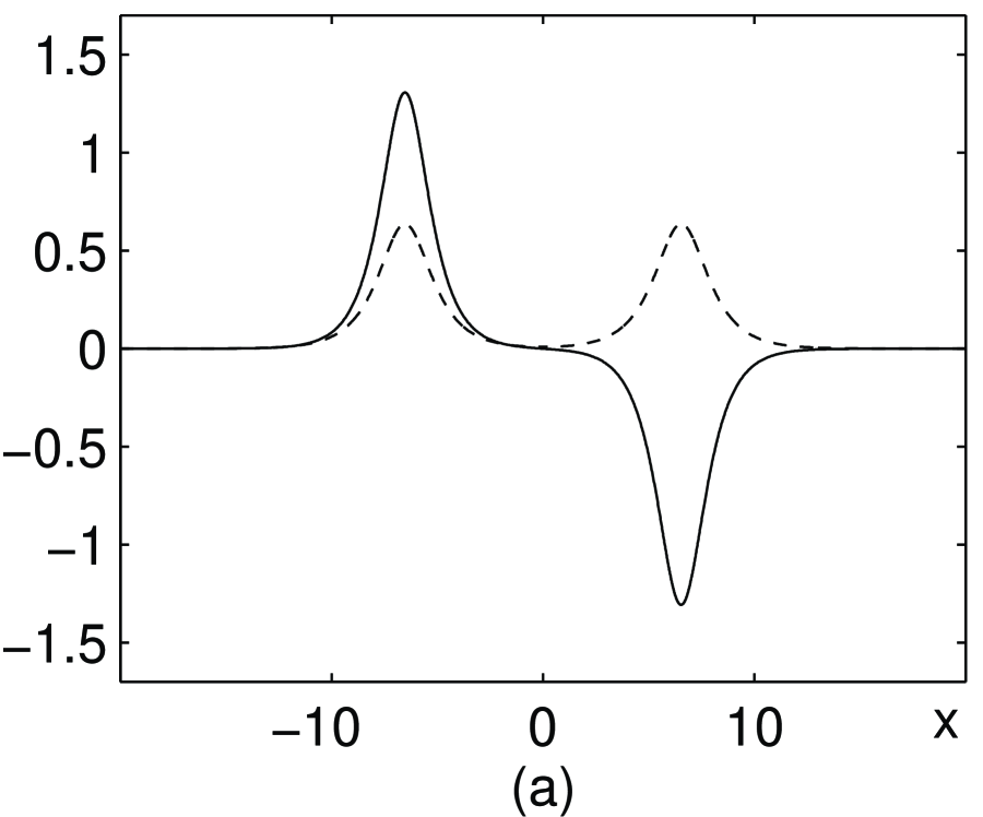
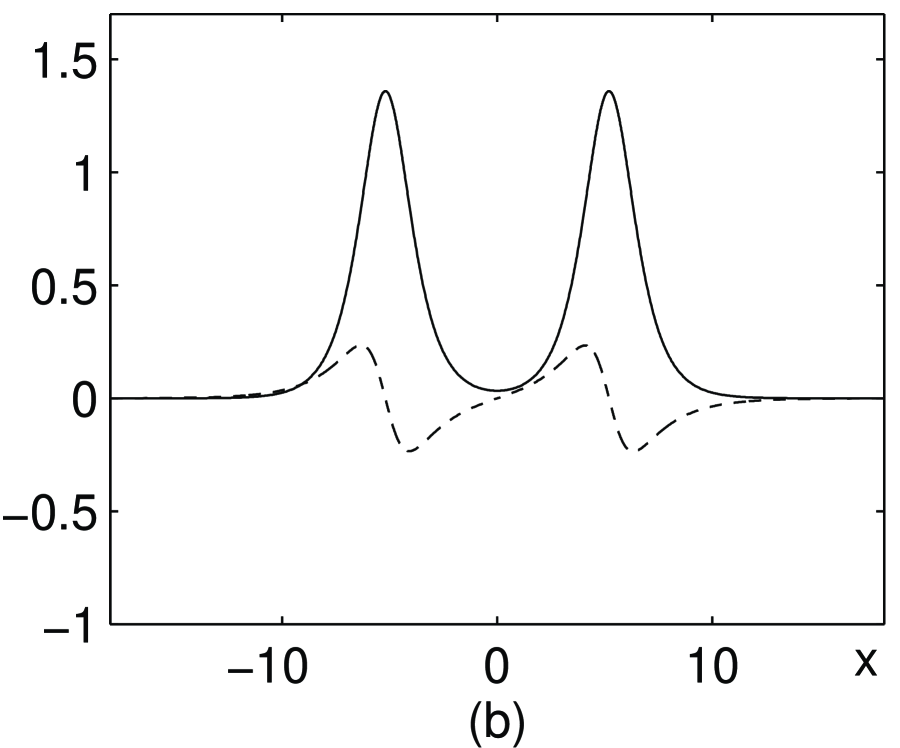
Figure 1: Solitary waves matched by two wave and daughter wave solutions. The solid curves are $r_{1}(x)$, and the dashed curves are $r_{2}(x)$. In (a), $(\beta,\omega)=(2/3,0.85)$ which is close to the curve (3.29) with $m=0$; in (b), $(\beta,\omega)=(2,0.6)$ which is close to the curve (3.29) with $m=1$.

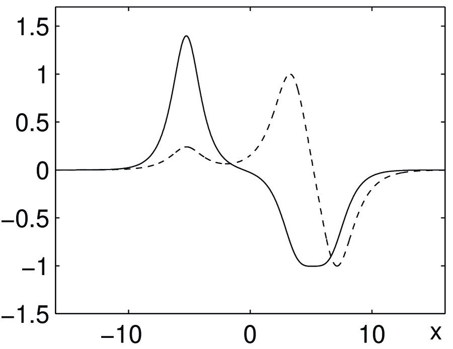
Figure 2: A solitary wave formed by mixed matching between a wave and daughter wave solution and another solitary wave of different type. Here $(\beta,\omega)=(2/3,0.78)$, close to curve (3.29) with $m=0$. The solid curve is $r_{1}(x)$, and the dashed curve is $r_{2}(x)$.

References

- [1] Ablowitz, M.J. and Segur, H. “Solitons and the inverse scattering transform.” SIAM, Philadelphia [1981].
- [2] Yang, J. “Classification of the solitary waves in coupled nonlinear Schrödinger equations.” Submitted to Physica D.
- [3] Balmforth, N.J. “Solitary waves and homoclinic orbits.” Annu. Rev. Fluid Mech. 27, 335 [1995].
- [4] Buffoni, B. and Séré, E. “A global condition for quasi-random behavior in a class of conservative systems.” Comm. Pure. Appl. Math. Vol. XLIX, 285 [1996].
- [5] Kalies, W.D. and VanderVorst, R.C.A.M. “Multitransition homoclinic and heteroclinic solutions of the extended Fisher-Kolmogorov equations.” CDSNS Report 95-231, Georgia Institute of Technology [1995].
- [6] Klauder, M., Laedke, E.W., Spatschek, K.H. and Turitsyn, S.K. “Pulse propagation in optical fibers near the zero dispersion point.” Phys. Rev. E 47, R3844 [1993].
- [7] Calvo, D.C. and Akylas, T.R. “On the formation of bound states by interacting nonlocal solitary waves.” Preprint [1996].
- [8] Karpman, V.I. and Solov’ev, V.V. “A perturbation theory for soliton systems.” Physica D 3, 142 [1981].
- [9] Gorshkov, K.A. and Ostrovsky, L.A. “Interactions of solitons in nonintegrable systems: direct perturbation method and applications.” Physica D 3, 428 [1981].
- [10] Benney, D.J. and Newell, A.C. “The propagation of nonlinear wave envelopes.” J. Math. and Phys. 46, 133 [1967].
- [11] Menyuk, C. R. “Nonlinear pulse propagation in birefringent optical fibers.” IEEE J. Quantum Electron, QE-23, 174 [1987].
- [12] Agrawal, G.P. “Nonlinear Fiber Optics.” Academic Press [1995].
- [13] Malomed, B.A. “Bound solitons in the nonlinear Schrödinger-Ginzburg-Landau equation.” Phys. Rev. A 44, 6954 [1991].
- [14] Malomed, B.A. “Bound solitons in coupled nonlinear Schrödinger equations.” Phys. Rev. A 45, R8321 [1992].
- [15] Kolodner, P. “Collisions between pulses of traveling-wave convection.” Phys. Rev. A 44, 6466 [1991].
- [16] Brand, H. and Deissler, R.J. “Interaction of localized solutions for subcritical bifurcations.” Phys. Rev. Lett. 63, 2801 [1989].