Instabilities of multi-hump vector solitons
in coupled nonlinear Schrödinger equations

Abstract

Spectral stability of multi-hump vector solitons in the Hamiltonian system of coupled nonlinear Schrödinger (NLS) equations is investigated both analytically and numerically. Using the closure theorem for the negative index of the linearized Hamiltonian, we classify all possible bifurcations of unstable eigenvalues in the systems of coupled NLS equations with cubic and saturable nonlinearities. We also determine the eigenvalue spectrum numerically by the shooting method. In case of cubic nonlinearities, all multi-hump vector solitons in the non-integrable model are found to be linearly unstable. In case of saturable nonlinearities, stable multi-hump vector solitons are found in certain parameter regions, and some errors in the literature are corrected.

1 Introduction

The coupled NLS equations have wide applications in the modeling of physical processes. For instance, such equations with the cubic nonlinearity govern the nonlinear interaction of two wave packets [4] and optical pulse propagation in birefringent fibers [23] or wavelength-division-multiplexed optical systems [1, 15]. Similar equations with the saturable nonlinearity describe the propagation of several mutually-incoherent laser beams in biased photorefractive crystals [11, 16]. Various types of vector solitons including single-hump and multi-hump ones have been known to exist in these coupled NLS equations [2, 3, 9, 10, 11, 14, 16, 25, 33, 34, 36], and they have been observed in photorefractive crystals as well [6, 7, 24].

Linear stability of vector solitons in the coupled NLS equations is an important issue. Fundamental single-hump vector solitons are known to be stable [26, 29, 37]. Stability of multi-hump vector solitons (which have one or more nodal points in one or more components) is more subtle. For the cubic nonlinearity, it was conjectured in [36] based on the numerical evidence that multi-hump vector solitons were all linearly unstable. If the multi-hump solitons are pieced together by a few fundamental vector solitons, then their linear instability has been proven both analytically and numerically in [38, 40]. The linear instability for other types of multi-hump vector solitons has not been proven yet. For the saturable nonlinearity, multi-hump solitons have been shown to be stable in certain parameter regions [25, 26], but the origins of their stability and instability have not yet been fully analyzed.

¿From a broader point of view, the theory of linear stability of vector solitons in coupled NLS equations was recently developed with the use of the closure theorem for the negative index of the linearized Hamiltonian [18, 27]. However, there are not many applications of the general theory to particular bifurcations of unstable eigenvalues [17, 41], because the general theory excludes non-generic bifurcations. It is desirable to further develop a perturbation theory to the eigenvalue bifurcations, so that the origin of instability becomes more apparent in the context of the closure theorem.

In this paper, we investigate the linear stability of multi-hump vector solitons in the general Hamiltonian system of coupled NLS equations both analytically and numerically. Using the closure theorem for the negative index of the linearized Hamiltonian as well as the perturbation technique, we classify all possible bifurcations of unstable eigenvalues in two physical models with cubic or saturable nonlinearities. In the first model, we show that multi-hump vector solitons near points of local bifurcations are always linearly unstable, in agreement with numerical results in [36]. In the second model, the situation is more complicated. Our results show that the 1st family of multi-hump vector solitons is indeed linearly stable near the local-bifurcation boundary, in agreement with numerical results in [26]. However, for the 2nd family, we discovered a new oscillatory instability near the local-bifurcation boundary, which was missed in [26]. Due to this oscillatory instability, the stability region of vector solitons for the 2nd family is drastically reduced from that reported in [26]. Numerically, we track the unstable eigenvalues of multi-hump solitons and reveal various scenarios of eigenvalue bifurcations away from the local-bifurcation boundaries. We also map out the correct stability regions of multi-hump vector solitons in the entire parameter space. Furthermore, the number of numerically-obtained unstable eigenvalues agrees completely with that predicted by the negative index of the linearized Hamiltonian.

Our paper is structured as follows. The main formalism and the closure theorem for the negative index of the linearized Hamiltonian are described in Section 2. Analysis of unstable eigenvalues in the coupled NLS equations with cubic and saturable nonlinearities is developed in Sections 3 and 4, respectively. Section 5 summarizes our results and open questions. Appendix A reviews bifurcations of unstable eigenvalues by the perturbation method.

2 Main formalism

We consider a general Hamiltonian system of coupled NLS equations in the form:

$$i\frac{\partial\psi_{n}}{\partial z}+d_{n}\frac{\partial^{2}\psi_{n}}{\partial x^{2}}+\frac{\partial U}{\partial|\psi_{n}|^{2}}\psi_{n}=0,\;\;\;\;n=1,...,N,$$ (2.1)

where $z\in\mathbb{R}_{+}$, $x\in\mathbb{R}$, $\psi_{n}\in\mathbb{C}$, $d_{n}\in\mathbb{R}$, and $U=U(|\psi_{1}|^{2},...,|\psi_{N}|^{2})\in\mathbb{R}$. We assume that $U(0)=U^{\prime}(0)=0$, and $d_{n}>0$ for all $n$. In optical fibers (photorefractive crystals), the function $\psi_{n}(z,x)$ is the envelope amplitude of the $n^{\rm th}$ channel (beam), $z$ is the propagation distance along the fiber (waveguide), and $x$ is the retarded time (the transverse coordinate) [11, 15, 16, 23].

Following the recent work in [27], we study the linear stability of vector solitons:

$$\psi_{n}(z,x)=\Phi_{n}(x)e^{i\beta_{n}z},$$ (2.2)

where $\Phi_{n}:\mathbb{R}\rightarrow\mathbb{R}$, and $\beta_{n}>0$ for all $n$. We assume that none of the components $\Phi_{n}(x)$ vanish identically on $x\in\mathbb{R}$. Linearization of the coupled NLS equations (2.1) follows from the expansion:

$$\psi_{n}(z,x)=\left\{\Phi_{n}(x)+\left[u_{n}(x)+iw_{n}(x)\right]e^{\lambda z}+\left[\bar{u}_{n}(x)+i\bar{w}_{n}(x)\right]e^{\bar{\lambda}z}\right\}e^{i\beta_{n}z},$$ (2.3)

where $\|u_{n}\|,\|w_{n}\|\ll 1$, and the overline denotes the complex conjugation. The linearized equations for $(u_{n},w_{n})$ are the following non-self-adjoint problem in $L^{2}(\mathbb{R},\mathbb{C}^{2N})$:

$${\cal L}_{1}{\bf u}=-\lambda{\bf w},\qquad{\cal L}_{0}{\bf w}=\lambda{\bf u},$$ (2.4)

where $\lambda\in\mathbb{C}$ is an eigenvalue, $({\bf u},{\bf w})^{T}:\mathbb{R}\rightarrow\mathbb{C}^{2N}$ is the eigenvector, and ${\cal L}_{0}$ and ${\cal L}_{1}$ are the matrix Schrödinger operators with elements:

$$({\cal L}_{0})_{n,m} = \left(-d_{n}\frac{d^{2}}{dx^{2}}+\beta_{n}-\frac{\partial U}{\partial\Phi_{n}^{2}}\right)\delta_{n,m},$$ (2.5)

$$({\cal L}_{1})_{n,m} = \left(-d_{n}\frac{d^{2}}{dx^{2}}+\beta_{n}-\frac{\partial U}{\partial\Phi_{n}^{2}}\right)\delta_{n,m}-2\frac{\partial^{2}U}{\partial\Phi_{n}^{2}\partial\Phi_{m}^{2}}\Phi_{n}\Phi_{m}.$$ (2.6)

Since the eigenvalue problem (2.4) is a linearization of the Hamiltonian system, the values of $\lambda$ occur as pairs of real or purely imaginary eigenvalues, or as quadruplets of complex eigenvalues. Eigenvalues with ${\rm Re}(\lambda)>0$ lead to spectral instability of vector solitons (2.2). We denote the number of eigenvalues in the first open quadrant as $N_{\rm comp}$, the number of positive real eigenvalues as $N_{\rm real}$, and the number of purely imaginary eigenvalues with positive ${\rm Im}(\lambda)$ as $N_{\rm imag}$. The continuous spectrum has $N$ branches, located at the positive imaginary axis for ${\rm Im}(\lambda)\geq\beta_{n}$, $n=1,...,N$. Zero eigenvalue $\lambda=0$ has geometric multiplicity of at least $(N+1)$ and algebraic multiplicity of at least $(2N+2)$, in the assumption that none of the components $\Phi_{n}(x)$ vanishes identically on $x\in\mathbb{R}$ [27].

Furthermore, we denote the number of negative and zero eigenvalues of operators ${\cal L}_{0,1}$ in $L^{2}(\mathbb{R},\mathbb{C}^{N})$ as $n({\cal L}_{0,1})$ and $z({\cal L}_{0,1})$, respectively. We also assume that the solution $\Phi_{n}(x)$ depends smoothly on $(\beta_{1},...,\beta_{N})$ in an open non-empty set of $\mathbb{R}^{N}$ and introduce the Hessian matrix ${\cal U}$ with elements:

$${\cal U}_{n,m}=\frac{\partial Q_{n}}{\partial\beta_{m}},$$ (2.7)

where $Q_{n}=Q_{n}(\beta_{1},...,\beta_{N})=\int_{\mathbb{R}}\Phi_{n}^{2}dx$. We denote the number of positive and zero eigenvalues of matrix ${\cal U}$ as $p({\cal U})$ and $z({\cal U})$, respectively. Finally, we introduce the linearized Hamiltonian (”energy”) of the eigenvalues $\lambda$ in $H^{1}(\mathbb{R},\mathbb{C}^{2N})$:

$$h[{\bf u},{\bf w}]=\langle{\bf u},{\cal L}_{1}{\bf u}\rangle+\langle{\bf w},{\cal L}_{0}{\bf w}\rangle,$$ (2.8)

where $\langle\cdot,\cdot\rangle$ is the standard inner product in $L^{2}(\mathbb{R},\mathbb{C}^{2N})$. The negative index of the linearized Hamiltonian is the number of negative eigenvalues of ${\cal L}_{1}$ and ${\cal L}_{0}$ in $L^{2}(\mathbb{R},\mathbb{C}^{N})$.

Several assumptions are imposed on the linearized problem (2.4) in a general case [27]:
          (i) $z({\cal L}_{1})=1$, $z({\cal L}_{0})=N$;
          (ii) $z({\cal U})=0$;
          (iii) no eigenvalues $\lambda\in i\mathbb{R}$ exist with $h[{\bf u},{\bf w}]=0$;
          (iv) no embedded eigenvalues $\lambda\in i\mathbb{R}$ exist with $|{\rm Im}(\lambda)|\geq\beta_{\rm min}$, where $\beta_{\rm min}=\min(\beta_{1},...,\beta_{N}).$

Closure Theorem [27] Assume that (i)–(iv) be satisfied. Let $N_{\rm imag}^{-}$ be the number of eigenvalues $\lambda\in i\mathbb{R}_{+}$ with $h[{\bf u},{\bf w}]<0$. Then

$$(i)\quad N_{\rm real}+2N_{\rm comp}+2N_{\rm imag}^{-}=n({\cal L}_{1})-p({\cal U})+n({\cal L}_{0}),$$ (2.9)

$$(ii)\quad N_{\rm real}\geq|n({\cal L}_{1})-p({\cal U})-n({\cal L}_{0})|,$$ (2.10)

$$(iii)\quad N_{\rm comp}\leq\min\left(n({\cal L}_{0}),n({\cal L}_{1})-p({\cal U})\right),$$ (2.11)

such that

$$|n({\cal L}_{1})-p({\cal U})-n({\cal L}_{0})|\leq N_{\rm unst}\leq n({\cal L}_{1})-p({\cal U})+n({\cal L}_{0}),$$ (2.12)

where $N_{\rm unst}=N_{\rm real}+2N_{\rm comp}$ is the total number of unstable eigenvalues in the problem (2.4).

This theorem was originally proved for the coupled NLS equations (2.1) in one dimension [27] and then generalized to a three-dimensional NLS equation [8] and to an abstract Hamiltonian dynamical system [18]. It allows us to analytically trace unstable eigenvalues under parameter continuations, starting with the particular limits, where all eigenvalues $\lambda$ of negative energy $h[{\bf u},{\bf w}]$ are known. Examples of such parameter continuation are recently reported in [17, 41] in the context of the coupled NLS equations.

Bifurcations of unstable eigenvalues may occur in the linearized problem (2.4), when operators ${\cal L}_{1}$ and ${\cal L}_{0}$ change according to a continuous deformation and one of the assumptions (i)–(iv) of the Closure Theorem fails. Bifurcations are reviewed in Appendix A. In what follows, we apply parameter continuation and bifurcation analysis to the system of coupled NLS equations (2.1) with cubic and saturable nonlinearities.

3 The coupled cubic NLS equations

We consider the system of coupled cubic NLS equations [4, 15, 23]:

$$i\psi_{1z}+\psi_{1xx}+\left(|\psi_{1}|^{2}+\chi|\psi_{2}|^{2}\right)\psi_{1} = 0,$$

$$i\psi_{2z}+\psi_{2xx}+\left(\chi|\psi_{1}|^{2}+|\psi_{2}|^{2}\right)\psi_{2} = 0,$$ (3.1)

where $\chi>0$. The system is a particular example of (2.1) with $N=2$, $d_{1}=d_{2}=1$, and

$$U=\frac{1}{2}|\psi_{1}|^{4}+\chi|\psi_{1}|^{2}|\psi_{2}|^{2}+\frac{1}{2}|\psi_{2}|^{4}.$$ (3.2)

The system (3.1) has a countable infinite set of families of vector solitons ${\bf\Phi}(x)=(\Phi_{1},\Phi_{2})^{T}$, classified by different nodal index ${\bf i}=(i_{1},i_{2})^{T}$, where $i_{n}$ is the number of zeros of $\Phi_{n}(x)$ on $x\in\mathbb{R}$ [9, 14, 36]. We consider here families of vector solitons with nodal index ${\bf i}=(0,n)^{T}$, $n\in\mathbb{N}$, which are locally close to the NLS soliton, ${\bf\Phi}_{\rm NLS}(x)=(\Phi^{(0)},0)^{T}$, where $\Phi^{(0)}(x)=\sqrt{2\beta_{1}}\;{\rm sech}(\sqrt{\beta_{1}}x)$. We let $\beta_{1}=1$ and $\beta_{2}=\beta$ for convenience and introduce scalar Schrödinger operators:

$$L_{0} = -\frac{d^{2}}{dx^{2}}+1-2\;{\rm sech}^{2}(x),$$ (3.3)

$$L_{1} = -\frac{d^{2}}{dx^{2}}+1-6\;{\rm sech}^{2}(x),$$ (3.4)

$$L_{s} = -\frac{d^{2}}{dx^{2}}+\lambda_{n}^{2}(\chi)-2\chi\;{\rm sech}^{2}(x),$$ (3.5)

where

$$\lambda_{n}(\chi)=\frac{\sqrt{1+8\chi}-(2n+1)}{2}.$$ (3.6)

The scalar operators $L_{0}$,$L_{1}$,$L_{s}$ define the matrix operators ${\cal L}_{0}$ and ${\cal L}_{1}$ at $\epsilon=0$:

$${\cal L}_{0}={\rm diag}(L_{0},L_{s}),\qquad{\cal L}_{1}={\rm diag}(L_{1},L_{s}).$$

We define the perturbation series expansions of vector solitons ${\bf\Phi}=(\Phi_{1},\Phi_{2})^{T}$:

$$\Phi_{1}(x) = \Phi^{(0)}(x)+\epsilon^{2}\Phi^{(2)}(x)+{\rm O}(\epsilon^{4}),$$

$$\Phi_{2}(x) = \epsilon\Phi^{(1)}(x)+\epsilon^{3}\Phi^{(3)}(x)+{\rm O}(\epsilon^{5}),$$ (3.7)

and

$$\beta=\lambda_{n}^{2}(\chi)+\epsilon^{2}C_{n}(\chi)+{\rm O}(\epsilon^{4}).$$ (3.8)

Corrections of the perturbation series (3.7)–(3.8) satisfy the linear equations:

$$L_{s}\Phi^{(1)} = 0,$$ (3.9)

$$L_{1}\Phi^{(2)} = \chi\Phi^{(0)}\left(\Phi^{(1)}\right)^{2},$$ (3.10)

$$L_{s}\Phi^{(3)} = -C_{n}(\chi)\Phi^{(1)}+2\chi\Phi^{(0)}\Phi^{(1)}\Phi^{(2)}+\left(\Phi^{(1)}\right)^{3}.$$ (3.11)

The problem (3.9) has a decaying solution $\Phi^{(1)}\equiv\Phi^{(1)}_{n}(x)$ (see [14, 36]). When $n=0$ and $\chi>0$, the solution $\Phi^{(1)}_{0}={\rm sech}^{s}(x)$, $s=\lambda_{0}(\chi)$ is a ground state. When $n>0$ and $\chi>\chi_{n}=n(n+1)/2$, the solution $\Phi^{(1)}_{n}(x)$ is an excited state with exactly $n$ nodes on $x\in\mathbb{R}$. The problem (3.10) also has a decaying solution $\Phi^{(2)}(x)$, since the right-hand-side $\chi\Phi^{(0)}\left(\Phi^{(1)}_{n}\right)^{2}$ is orthogonal to the kernel of the operator ${\cal L}_{1}$, which is $\Phi^{(0)\prime}(x)$. By the Fredholm Alternative Theorem, the problem (3.11) has a decaying solution if and only if the right-hand-side is orthogonal to the kernel of ${\cal L}_{s}$, which is $\Phi^{(1)}_{n}(x)$. The orthogonality condition defines the parameter $C_{n}(\chi)$ in the form:

$$C_{n}(\chi)=\frac{\langle\left(\Phi^{(1)}_{n}\right)^{2},\left(2\chi\Phi^{(0)}\Phi^{(2)}+\left(\Phi^{(1)}_{n}\right)^{2}\right)\rangle}{\langle\Phi^{(1)}_{n},\Phi^{(1)}_{n}\rangle}.$$ (3.12)

The condition $C_{n}(\chi)\neq 0$ gives the sufficient condition of continuation of the perturbation series expansions (3.7)–(3.8). Thus, for $\chi>\chi_{n}$ and $C_{n}(\chi)\neq 0$, there exists some $R_{n}>0$, such that the $n$-th family of vector solitons ${\bf\Phi}(x)=(\Phi_{1},\Phi_{2})^{T}$ with the nodal index ${\bf i}=(0,n)^{T}$ bifurcates from ${\bf\Phi}_{\rm NLS}=(\Phi^{(0)},0)^{T}$ in the one-sided domain ${\cal B}_{n}$:

$${\cal B}_{n}=\left\{\beta:0<\left|\beta-\lambda_{n}^{2}(\chi)\right|<R_{n},\quad{\rm sign}\left(\beta-\lambda_{n}^{2}(\chi)\right)={\rm sign}(C_{n}(\chi))\right\}.$$ (3.13)

These results for the first three families $n=0,1,2$ were analytically obtained and numerically verified in [36]. We investigate stability of the $n$-th family of vector solitons in the one-sided domain ${\cal B}_{n}$ below.

3.1 Analytical results

We trace unstable eigenvalues using the Closure Theorem. We consider a generic case $C_{n}(\chi)\neq 0$ in the one-sided open domain ${\cal B}_{n}$ and show that the left-hand and right-hand sides of the closure relation (2.9) are equal to $2n$ for small $\epsilon\geq 0$.

Operator $L_{0}$ in (3.3) has one bound state for zero eigenvalue, operator $L_{1}$ in (3.4) has two bound states for negative and zero eigenvalues, and operator $L_{s}$ in (3.5) has $(n+1)$ bound states with $n$ negative and one zero eigenvalues. Therefore, at $\epsilon=0$, we have $n({\cal L}_{0})=0+n=n$, $z({\cal L}_{0})=1+1=2$, $n({\cal L}_{1})=1+n$ and $z({\cal L}_{1})=1+1=2$. It follows from Sturm Nodal Theorem that

$$n({\cal L}_{0})=n,\qquad z({\cal L}_{0})=2,\qquad\forall\epsilon\geq 0.$$

Since $z({\cal L}_{1})=2>1$, we have the bifurcation case $z({\cal L}_{1})>1$ for $\epsilon=0$ (see Appendix A.1). It is however a degenerate bifurcation case, since it occurs on the boundary of the existence domain ${\cal B}_{n}$, such that $\beta\in\partial{\cal B}_{n}$. We trace the zero eigenvalue of ${\cal L}_{1}$ for $\epsilon\neq 0$ by the regular perturbation series,

$${\bf u}(x)=\left[\begin{array}[]{c}0\\ \Phi^{(1)}_{n}(x)\end{array}\right]+\epsilon\left[\begin{array}[]{c}u^{(1)}(x)\\ 0\end{array}\right]+\epsilon^{2}\left[\begin{array}[]{c}0\\ u^{(2)}(x)\end{array}\right]+{\rm O}(\epsilon^{3})$$ (3.20)

and

$$\lambda=\epsilon^{2}\lambda_{2}+{\rm O}(\epsilon^{4}).$$ (3.21)

Corrections of the perturbation series (3.20) satisfy a set of linear non-homogeneous equations:

$$L_{1}u^{(1)} = 2\chi\Phi^{(0)}\left(\Phi^{(1)}_{n}\right)^{2},$$ (3.22)

$$L_{s}u^{(2)} = (\lambda_{2}-C_{n}(\chi))\Phi^{(1)}_{n}+2\chi\Phi^{(0)}\Phi^{(1)}_{n}\left(u^{(1)}+\Phi^{(2)}\right)+3\left(\Phi^{(1)}_{n}\right)^{3}.$$ (3.23)

It follows from (3.10) and (3.22) that $u^{(1)}=2\Phi^{(2)}$. By the Fredholm Alternative Theorem, decaying solutions of (3.23) exist if and only if the right-hand-side of (3.23) is orthogonal to $\Phi^{(1)}_{n}(x)$. Using (3.12), we find that $\lambda_{2}=-2C_{n}(\chi)$. Therefore, we have:

$$n({\cal L}_{1})=1+\Theta(C_{n}(\chi))+n,\qquad z({\cal L}_{1})=1,\qquad\epsilon>0,$$

where $\Theta(z)$ is the Heaviside step-function. We trace the zero eigenvalue of ${\cal U}$ from (2.7) and (3.7):

$${\cal U}_{1,1} = \frac{\partial Q_{1}}{\partial\beta_{1}}\biggr{|}_{\beta_{1}=1}=2+2\langle\Phi^{(0)},\Phi^{(2)}\rangle\frac{\partial\epsilon^{2}}{\partial\beta_{1}}\biggr{|}_{\beta_{1}=1}+{\rm O}(\epsilon^{2}),$$

$${\cal U}_{1,2} = \frac{\partial Q_{1}}{\partial\beta_{2}}\biggr{|}_{\beta_{1}=1}=2\langle\Phi^{(0)},\Phi^{(2)}\rangle\frac{\partial\epsilon^{2}}{\partial\beta_{2}}\biggr{|}_{\beta_{1}=1}+{\rm O}(\epsilon^{2}),$$

$${\cal U}_{2,1} = \frac{\partial Q_{2}}{\partial\beta_{1}}\biggr{|}_{\beta_{1}=1}=\langle\Phi^{(1)}_{n},\Phi^{(1)}_{n}\rangle\frac{\partial\epsilon^{2}}{\partial\beta_{1}}\biggr{|}_{\beta_{1}=1}+{\rm O}(\epsilon^{2}),$$

$${\cal U}_{2,2} = \frac{\partial Q_{2}}{\partial\beta_{2}}\biggr{|}_{\beta_{1}=1}=\langle\Phi^{(1)}_{n},\Phi^{(1)}_{n}\rangle\frac{\partial\epsilon^{2}}{\partial\beta_{2}}\biggr{|}_{\beta_{1}=1}+{\rm O}(\epsilon^{2}).$$

It follows from (3.8) that

$$\frac{\partial\epsilon^{2}}{\partial\beta_{2}}\biggr{|}_{\beta_{1}=1}=\frac{1}{C_{n}(\chi)}+{\rm O}(\epsilon^{2})$$ (3.24)

and, due to the symmetry of ${\cal U}$,

$$\det({\cal U})=\frac{2\langle\Phi^{(1)}_{n},\Phi^{(1)}_{n}\rangle}{C_{n}(\chi)}+{\rm O}(\epsilon^{2}).$$ (3.25)

Therefore, we have:

$$p({\cal U})=1+\Theta(C_{n}(\chi)),\qquad z({\cal U})=0,\qquad\epsilon>0.$$

We conclude that the bifurcation case $z({\cal L}_{1})>1$ on the boundary of the existence domain $\beta\in\partial{\cal B}_{n}$ does not result in bifurcation of any eigenvalue $\lambda$ of the stability problem (2.4), such that $n({\cal L}_{1})-p({\cal U})+n({\cal L}_{0})=2n$ is valid everywhere in $\beta\in{\cal B}_{n}\cup\partial{\cal B}_{n}$. It follows from the Closure Theorem that the ground state with $n=0$ is spectrally stable in $\beta\in{\cal B}_{n}$, while the $n$-th excited state with $n\geq 1$ may have at most $N_{\rm unst}$ unstable eigenvalues, where $0\leq N_{\rm unst}\leq 2n$. We show that $N_{\rm unst}=2N_{\rm comp}=2n$ in $\beta\in{\cal B}_{n}$ in a generic case.

At $\epsilon=0$, the stability problem (2.4) can be decoupled as follows:

$$L_{1}u_{1}=-\lambda w_{1},\qquad L_{0}w_{1}=\lambda u_{1}$$ (3.26)

and

$$L_{s}(u_{2}\pm iw_{2})=\pm i\lambda(u_{2}\pm iw_{2}).$$ (3.27)

The first problem (3.26) has the continuous spectrum for ${\rm Re}(\lambda)=0$ and $|{\rm Im}(\lambda)|\geq 1$ and the zero eigenvalue $\lambda=0$ of algebraic multiplicity 4 and geometric multiplicity 2. The second problem (3.27) has the continuous spectrum for ${\rm Re}(\lambda)=0$ and $|{\rm Im}(\lambda)|\geq\lambda_{n}^{2}(\chi)$, zero eigenvalue $\lambda=0$ of geometric and algebraic multiplicity 2, and $2n$ isolated eigenvalues in the points $\lambda=\pm i\left(\lambda_{k}^{2}-\lambda_{n}^{2}\right)$, where $k=0,1,...,n-1$. It follows from (3.6) that for $\chi>\chi_{n}$:

$$\lambda_{k}^{2}-\lambda_{n}^{2}=(n-k)\left[2\lambda_{n}(\chi)+(n-k)\right]>(n-k)^{2}\geq 1,\qquad 0\leq k<n.$$ (3.28)

Therefore, $2n$ isolated eigenvalues of the problem (3.27) are embedded in the continuous spectrum of the problem (3.26). These embedded eigenvalues have negative energy $h[{\bf u},{\bf w}]$, since at $\epsilon=0$:

$$\langle{\bf u}_{k},{\cal L}_{1}{\bf u}_{k}\rangle=\langle{\bf w}_{k},{\cal L}_{0}{\bf w}_{k}\rangle=-(\lambda_{k}^{2}-\lambda_{n}^{2})\langle\Phi_{k}^{(1)},\Phi_{k}^{(1)}\rangle,\qquad 0\leq k<n,$$ (3.29)

where ${\bf u}_{k}=(0,\Phi_{k}^{(1)})^{T}$ and ${\bf w}_{k}=(0,\mp i\Phi_{k}^{(1)})^{T}$ at $\epsilon=0$. By Appendix A.4, all $2n$ embedded eigenvalues of negative energy $h[{\bf u},{\bf w}]$ bifurcate in a general case of non-zero $\Gamma$, see Eq. (A.29), to complex unstable eigenvalues $\lambda\in\mathbb{C}$, ${\rm Re}(\lambda)>0$ for $\epsilon\neq 0$, such that $N_{\rm real}+2N_{\rm comp}+2N_{\rm imag}^{-}=2N_{\rm comp}=2n$ in $\beta\in{\cal B}_{n}$.

3.2 Numerical results

For $\epsilon\neq 0$, the linearized problem (2.4) satisfies the assumptions of the Closure Theorem. Therefore, all unstable eigenvalues $N_{\rm unst}=2N_{\rm comp}=2n$ are structurally stable for larger values of $\epsilon$, until new bifurcations occur in the parameter continuations. We study numerically locations of unstable eigenvalues in the linearized problem (2.4) related to the vector solitons ${\bf\Phi}=(\Phi_{1},\Phi_{2})^{T}$ with nodal index ${\bf i}=(0,n)^{T}$, $n=1,2$. Our numerical algorithm is based on the shooting technique in the complex $\lambda$-plane. We also determine the indices $n({\cal L}_{0})$, $n({\cal L}_{1})$ and $p({\cal U})$ by a numerics-assisted procedure as described in [39], and relate them to the number of unstable eigenvalues by using the closure relation (2.9).

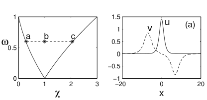
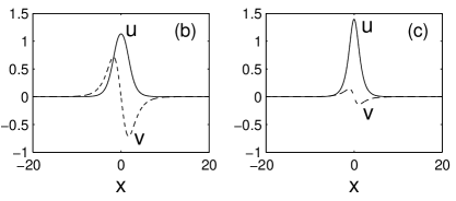
Figure 1: Vector solitons of the 1st-family in the cubic model (3) at $\beta=0.36$ and three $\chi$ values marked as ”*” in the upper left figure. Here $\omega\equiv\sqrt{\beta}$, and $(u,v)\equiv(\Phi_{1},\Phi_{2})$.

Figure 1 shows the 1st-family of multi-hump vector solitons with the correspondence: $u=\Phi_{1}(x)$, $v=\Phi_{2}(x)$, and $\omega=\sqrt{\beta}$. For $\omega<1$, this family exists between $\chi_{1}(\beta)<\chi<\chi_{2}(\beta)$, where $\chi=\chi_{2}(\beta)$ is the local bifurcation boundary, and $\chi=\chi_{1}(\beta)$ is the nonlocal bifurcation boundary [9]. Hence the one-sided domain $\beta\in{\cal B}_{1}$ is located to the left of the local bifurcation curve, and ${\rm sign}(C_{1})=1$ in (3.13). When parameter $\omega=0.6$ is fixed, we readily find that $\chi_{1}=0.28$ and $\chi_{2}=2.08$. When $\chi$ moves from $\chi_{2}$ to $\chi_{1}$, the distance between the two pulses in the $v$ component grows. It diverges to infinity at the nonlocal bifurcation boundary $\chi_{2}$ (near point $a$ in Fig. 1).

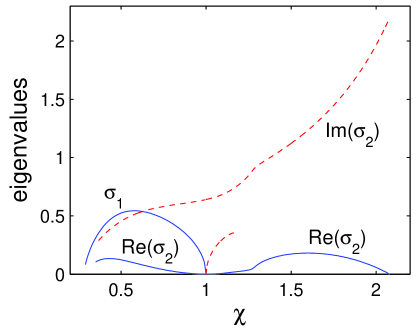
Figure 2: Eigenvalue spectrum of the 1st family of vector solitons in the cubic model (3) at $\beta=0.36$. The solid (dashed) lines are the real (imaginary) parts of the eigenvalues.

Figure 2 shows unstable eigenvalues of the linearized problem (2.4) for $\omega=0.6$ and $\chi_{1}<\chi<\chi_{2}$. In the domain $\beta\in{\cal B}_{1}$, there is a pair of unstable complex eigenvalues $\lambda={\rm Re}(\sigma_{2})\pm i{\rm Im}(\sigma_{2})$, which bifurcate from the embedded eigenvalues $\lambda=\pm i(\lambda_{0}^{2}-\lambda_{1}^{2})$, see Eq. (3.28).

When $\chi\to 1^{+}$, the complex eigenvalues $\lambda={\rm Re}(\sigma_{2})\pm i{\rm Im}(\sigma_{2})$ approach the imaginary axis and become embedded eigenvalues $\lambda=\pm i(1-\omega^{2})$. The case $\chi=1$ corresponds to the integrable Manakov system, when the linearized problem (2.4) has the following exact solution:

$${\bf u}_{0}=\left(\begin{array}[]{cc}-\Phi_{2}\\ \Phi_{1}\end{array}\right)\qquad{\bf w}_{0}=\mp i\left(\begin{array}[]{cc}\Phi_{2}\\ \Phi_{1}\end{array}\right),\qquad\lambda=\pm i(1-\omega^{2}).$$ (3.30)

This exact solution is generated by the additional polarizational-rotation symmetry in the potential function $U=U(|\psi_{1}|^{2}+|\psi_{2}|^{2})$ at $\chi=1$. Embedded eigenvalues $\lambda=\pm i(1-\omega^{2})$ have negative energy $h[{\bf u},{\bf w}]$, since

$$\langle{\bf u}_{0},{\cal L}_{1}{\bf u}_{0}\rangle=\langle{\bf w}_{0},{\cal L}_{0}{\bf w}_{0}\rangle=-(1-\omega^{2})\left(\langle\Phi_{1},\Phi_{1}\rangle-\langle\Phi_{2},\Phi_{2}\rangle\right)<0,$$ (3.31)

where the last inequality is confirmed numerically from integration of the exact solutions [34]:

$$\Phi_{1}(x) = \frac{\sqrt{1-\omega^{2}}\cosh\omega x}{\cosh x\cosh\omega x-\omega\sinh x\sinh\omega x},$$ (3.32)

$$\Phi_{2}(x) = -\frac{\omega\sqrt{1-\omega^{2}}\sinh x}{\cosh x\cosh\omega x-\omega\sinh x\sinh\omega x},$$ (3.33)

in the entire domain of existence: $0<\omega<1$. Since embedded eigenvalues $\lambda=\pm i(1-\omega^{2})$ at $\chi=1$ have negative energy $h[{\bf u},{\bf w}]$, they bifurcate to the complex plane for $\chi\neq 1$ when the polarizational symmetry is destroyed. This is indeed the case as shown in Fig. 2, in agreement with Appendix A.4.

There is an additional instability bifurcation at $\chi=1$. This bifurcation comes about because at this $\chi$ value, the 1st-family of vector solitons ${\bf\Phi}=(\Phi_{1},\Phi_{2})^{T}$ can be generalized to asymmetric solutions with an additional free parameter [3, 14, 36]. As a result, the derivative of the asymmetric vector solitons with respect to the free parameter is an eigenvector in the kernel of the operator ${\cal L}_{1}$, such that $z({\cal L}_{1})=2$ at $\chi=1$. When $\chi\neq 1$, the integrability of the Manakov system is destroyed, and a pair of real or purely imaginary eigenvalues is generated, in agreement with Appendix A.1. Indeed, Fig. 2 shows a pair of purely imaginary eigenvalues $\lambda=\pm i\sigma_{1}$ for $\chi>1$, which merge to the end points $\lambda=\pm i\omega^{2}$ of the continuous spectrum at $\chi=1.185$, and a pair of real eigenvalues $\lambda=\pm\sigma_{1}$ for $\chi<1$.

Now we relate results of Fig. 2 to the closure relation (2.9). For this purpose, we have determined the indices $n({\cal L}_{1})$ and $p({\cal U})$ by the numerics-assisted procedure in [39] (we note that $n({\cal L}_{0})=1$ everywhere in the existence domain of the 1st-family of vector solitons). For $\omega=0.6$, we have found numerically that

$$n({\cal L}_{1})=\left\{\begin{array}[]{c}4,\hskip 8.5359pt\chi_{1}<\chi<1,\\ 3,\hskip 8.5359pt1<\chi<\chi_{2},\end{array}\right.\qquad p({\cal U})=2,\;\mbox{for all $\chi_{1}<\chi<\chi_{2}$},$$ (3.34)

such that

$$n({\cal L}_{1})+n({\cal L}_{0})-p({\cal U})=\left\{\begin{array}[]{c}3,\hskip 8.5359pt\chi_{1}<\chi<1,\\ 2,\hskip 8.5359pt1<\chi<\chi_{2}.\end{array}\right.$$ (3.35)

On the other hand, Fig. 2 shows that

$$N_{\rm comp}=1,\;\mbox{for all $\chi_{1}<\chi<\chi_{2}$},\qquad N_{\rm real}=\left\{\begin{array}[]{c}1,\hskip 8.5359pt\chi_{1}<\chi<1\\ 0,\hskip 8.5359pt1<\chi<\chi_{2}\end{array}\right.$$ (3.36)

and the closure relation (2.9) is thus satisfied.

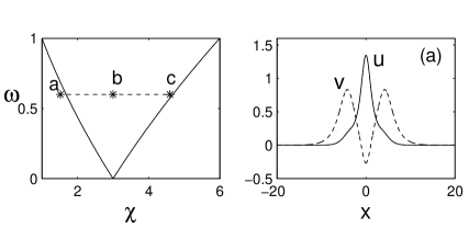
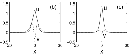
Figure 3: Vector solitons of the 2nd family in the cubic model (3) at $\beta=0.36$ and three $\chi$ values. Notations $\omega,u$ and $v$ are the same as in Fig. 1.

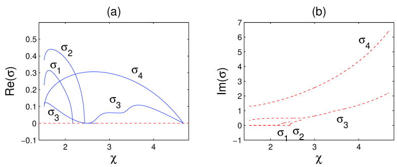
Figure 4: Eigenvalue spectrum of the 2nd family of vector solitons in the cubic model (3) at $\beta=0.36$. The solid (dashed) lines are the real (imaginary) parts of the eigenvalues.

Figures 3 and 4 show similar results for the 2nd family of multi-hump vector solitons. When parameter $\omega=0.6$ is fixed, the local bifurcation boundary is $\chi_{2}=4.68$ and the nonlocal bifurcation boundary is $\chi_{1}=1.68$. Again, the one-sided domain $\beta\in{\cal B}_{2}$ is located to the left of the local bifurcation boundary, such that ${\rm sign}(C_{2})=1$. However, such solitons exist on both sides of the nonlocal bifurcation boundary $\chi=\chi_{1}$. As $\chi$ moves leftward from $\chi=\chi_{2}$, it first crosses the nonlocal bifurcation boundary $\chi=\chi_{1}$, then turns around, and approaches the nonlocal bifurcation boundary from the left side (see point $a$ in Fig. 3). This behavior has been explained both analytically and numerically in [9].

Using the same shooting algorithm, we have obtained the unstable eigenvalues of the linearized problem (2.4) and displayed them in Fig. 4. In the domain $\beta\in{\cal B}_{2}$, there exist two pairs of unstable complex eigenvalues, such that the pair $\lambda={\rm Re}(\sigma_{4})\pm i{\rm Im}(\sigma_{4})$ bifurcates from the pair of embedded eigenvalues $\lambda=\pm i(\lambda_{0}^{2}-\lambda_{2}^{2})$, while the pair $\lambda={\rm Re}(\sigma_{3})\pm i{\rm Im}(\sigma_{3})$ bifurcates from the pair of embedded eigenvalues $\lambda=\pm i(\lambda_{1}^{2}-\lambda_{2}^{2})$. Fig. 4 also shows that the pair $\lambda={\rm Re}(\sigma_{3})\pm i{\rm Im}(\sigma_{3})$ approach the imaginary axis and become a pair of embedded eigenvalues at $\chi=\chi_{a}\approx 2.49$, but then reappear as a pair of complex unstable eigenvalues for $\chi<\chi_{a}$, in agreement with Appendix A.4.

There are two more instability bifurcations in Fig. 4. At $\chi=\chi_{b}\approx 2.44$, the zero eigenvalue bifurcates into a pair of imaginary eigenvalues $\lambda=\pm i\sigma_{2}$ for $\chi>\chi_{b}$, which then merge into the end points $\lambda=\pm i\omega^{2}$ of the continuous spectrum at $\chi\approx 2.72$. When $\chi<\chi_{b}$, this zero eigenvalue bifurcates into a pair of real unstable eigenvalues $\lambda=\pm\sigma_{2}$. At yet another point $\chi=\chi_{c}=2.17$, the zero eigenvalue bifurcates into a pair of imaginary eigenvalues $\lambda=\pm i\sigma_{1}$ for $\chi>\chi_{c}$, which merge into the end points $\lambda=\pm i\omega^{2}$ of the continuous spectrum at $\chi\approx 3.01$. When $\chi<\chi_{c}$, this zero eigenvalue bifurcates into a pair of real unstable eigenvalues $\lambda=\pm\sigma_{1}$.

To relate numerical results of Fig. 4 to the closure relation (2.9), we have again determined the indices $n({\cal L}_{1})$ and $p({\cal U})$ by the numerical algorithm, while $n({\cal L}_{0})=2$ everywhere in the existence domain of the 2nd family of vector solitons. For $\omega=0.6$, we have found numerically that

$$n({\cal L}_{1})=\left\{\begin{array}[]{c}5,\hskip 8.5359pt\chi_{1}<\chi<\chi_{b},\\ 4,\hskip 8.5359pt\chi_{b}<\chi<\chi_{2},\end{array}\right.\qquad p({\cal U})=\left\{\begin{array}[]{c}1,\hskip 8.5359pt\chi_{1}<\chi<\chi_{c},\\ 2,\hskip 8.5359pt\chi_{c}<\chi<\chi_{2},\end{array}\right.$$ (3.37)

such that

$$n({\cal L}_{1})+n({\cal L}_{0})-p({\cal U})=\left\{\begin{array}[]{l}6,\hskip 8.5359pt\chi_{1}<\chi<\chi_{c},\\ 5,\hskip 8.5359pt\chi_{c}<\chi<\chi_{b},\\ 4,\hskip 8.5359pt\chi_{b}<\chi<\chi_{2}.\end{array}\right.$$ (3.38)

On the other hand, Fig. 4 shows that

$$N_{\rm comp}=2,\;\mbox{for all $\chi_{1}<\chi<\chi_{2}$},\qquad N_{\rm real}=\left\{\begin{array}[]{l}2,\hskip 8.5359pt\chi_{1}<\chi<\chi_{c},\\ 1,\hskip 8.5359pt\chi_{c}<\chi<\chi_{b},\\ 0,\hskip 8.5359pt\chi_{b}<\chi<\chi_{2}.\end{array}\right.$$ (3.39)

Hence the closure relation (2.9) is satisfied. In particular, the instability bifurcation at $\chi=\chi_{b}$ is due to a jump in the index $n({\cal L}_{1})$ (similar to the 1st family), while the instability bifurcation at $\chi=\chi_{c}$ is due to a jump in the index $p({\cal U})$. These two bifurcations occur in agreement with Appendices A.1 and A.2.

Although our results were obtained here for a particular value $\omega=0.6$, we expect that similar results hold for other values of $\omega$, when $0<\omega<1$. We conclude that the 1st and 2nd families of multi-hump vector solitons in the coupled cubic NLS equations are all linearly unstable (except for the integrable Manakov system $\chi=1$, where the 1st family is neutrally stable).

It is remarkable that the main features of instability bifurcations for the 1st-family of multi-hump vector solitons are repeated for the 2nd-family of vector solitons, irrelevant whether the coupled NLS equations are integrable or not. This allows us to conjecture that a similar pattern of unstable eigenvalues persists for a general $n$-th family of multi-hump vector solitons, with more unstable eigenvalues and additional instability bifurcations appearing as $n$ increases.

4 Two coupled saturable NLS equations

We consider the system of two coupled saturable NLS equations [11, 16]:

$$i\psi_{1z}+\psi_{1xx}+\frac{|\psi_{1}|^{2}+|\psi_{2}|^{2}}{1+s(|\psi_{1}|^{2}+|\psi_{2}|^{2})}\psi_{1} = 0,$$

$$i\psi_{2z}+\psi_{2xx}+\frac{|\psi_{1}|^{2}+|\psi_{2}|^{2}}{1+s(|\psi_{1}|^{2}+|\psi_{2}|^{2})}\psi_{2} = 0,$$ (4.1)

where $s>0$. This system is a particular example of (2.1) with $N=2$, $d_{1}=d_{2}=1$, and

$$U=\frac{1}{s}\left(|\psi_{1}|^{2}+|\psi_{2}|^{2}\right)-\frac{1}{s^{2}}\log\left(1+s(|\psi_{1}|^{2}+|\psi_{2}|^{2})\right).$$ (4.2)

We consider again the $n$-th family of vector solitons ${\bf\Phi}=(\Phi_{1},\Phi_{2})^{T}$ with nodal index ${\bf i}=(0,n)^{T}$, $n\in\mathbb{N}$ and convenient parametrization $\beta_{1}=1$ and $\beta_{2}=\beta$. The $n$-th family bifurcates from the scalar solution ${\bf\Phi}=(\Phi_{0},0)^{T}$, where $\Phi_{0}(x)$ satisfies the ODE:

$$\Phi_{0}^{\prime\prime}-\Phi_{0}+\frac{\Phi_{0}^{3}}{1+s\Phi_{0}^{2}}=0.$$ (4.3)

The local bifurcation occurs at $\beta=\beta_{n}(s)$, when there exists a $n$-nodal bound state $\Phi_{n}(x)$ in the linear eigenvalue problem:

$$\Phi_{n}^{\prime\prime}-\beta_{n}\Phi_{n}+\frac{\Phi_{0}^{2}\Phi_{n}}{1+s\Phi_{0}^{2}}=0.$$ (4.4)

Vector solitons in the $n$-th family disappear at the nonlocal bifurcation boundary. The domain of existence for the first three families $n=0,1,2$ has been obtained numerically in [9, 26]. We trace analytically unstable eigenvalues and show that $N_{\rm real}+2N_{\rm comp}+2N_{\rm imag}^{-}=2n$ for small $|\beta-\beta_{n}(s)|\ll 1$. At $\beta=\beta_{n}(s)$, the stability problem (2.4) can be decoupled as follows:

$$L_{1}u_{1}=-\lambda w_{1},\qquad L_{0}w_{1}=\lambda u_{1}$$ (4.5)

and

$$L_{s}(u_{2}\pm iw_{2})=\pm i\lambda(u_{2}\pm iw_{2}),$$ (4.6)

where

$$L_{0} = -\frac{d^{2}}{dx^{2}}+1-\frac{\Phi_{0}^{2}}{1+s\Phi_{0}^{2}},$$ (4.7)

$$L_{1} = -\frac{d^{2}}{dx^{2}}+1-\frac{\Phi_{0}^{2}(3+s\Phi_{0}^{2})}{(1+s\Phi_{0}^{2})^{2}},$$ (4.8)

$$L_{s} = -\frac{d^{2}}{dx^{2}}+\beta_{n}(s)-\frac{\Phi_{0}^{2}}{1+s\Phi_{0}^{2}}.$$ (4.9)

The first problem (4.5) is the linearized stability problem in the scalar saturable NLS equation (4.1) for $\Phi_{0}(x)$. Based on numerical data in [25, 26], we assume that the bound state $\Phi_{0}(x)$ is spectrally stable in the scalar saturable NLS equation and the problem (4.5) does not have any eigenvalues of negative energy $h[{\bf u},{\bf w}]$. It has the continuous spectrum at ${\rm Re}(\lambda)=0$ and $|{\rm Im}(\lambda)|\geq 1$, the zero eigenvalue $\lambda=0$ of algebraic multiplicity 4 and geometric multiplicity 2, and possibly isolated eigenvalues $\lambda\in i\mathbb{R}$ of positive energy.

The second problem (4.6) has the continuous spectrum at ${\rm Re}(\lambda)=0$ and $|{\rm Im}(\lambda)|\geq\beta_{n}(s)$, zero eigenvalue $\lambda=0$ of geometric and algebraic multiplicity 2, and $2n$ isolated eigenvalues $\lambda=\pm i[\beta_{k}(s)-\beta_{n}(s)]$, where $k=0,1,...,n-1$. By the Sturm Nodal Theorem, eigenvalues $\beta_{k}(s)$ ($k=0,...,n$) are ordered in the decreasing order and are characterized by eigenfunctions $\Phi_{k}(x)$ with $k$ nodes, such that the ground state $\Phi_{0}(x)$ corresponds to $\beta_{0}(s)=1$ and the $n$-th excited state $\Phi_{n}(x)$ corresponds to $\beta_{n}(s)$. The $2n$ eigenvalues have negative energy $h[{\bf u},{\bf w}]$, since

$$\langle{\bf u}_{k},{\cal L}_{1}{\bf u}_{k}\rangle=\langle{\bf w}_{k},{\cal L}_{0}{\bf w}_{k}\rangle=-\left[\beta_{k}(s)-\beta_{n}(s)\right]\langle\Phi_{k},\Phi_{k}\rangle<0,\qquad 0\leq k<n,$$ (4.10)

where ${\bf u}_{k}=(0,\Phi_{k})^{T}$ and ${\bf w}_{k}=(0,\mp i\Phi_{k})^{T}$ at $\beta=\beta_{n}(s)$. Therefore, $2N_{\rm imag}^{-}=2n$ at $\beta=\beta_{n}(s)$. Since the zero eigenvalue has the generic algebraic multiplicity six, no negative eigenvalues of ${\cal L}_{1}$ and ${\cal L}_{0}$ arise from the zero eigenvalue, such that we have $N_{\rm real}+2N_{\rm comp}+2N_{\rm imag}^{-}=2n$ for $|\beta-\beta_{n}(s)|\ll 1$ by continuity of the negative index $n(h)$. The ground state with $n=0$ is therefore spectrally stable in the existence domain (which is $\beta=1$, $s>0$ for $n=0$).

We show that the nodal bound state with $n\geq 1$ may have at most $N_{\rm unst}$ unstable eigenvalues, where $0\leq N_{\rm unst}\leq 2n-2$. The number of unstable eigenvalues is reduced by two, since there are two eigenvalues $\lambda=\pm i(1-\beta)$ of negative energy, which exist for all vector solitons with $n\geq 1$ due to the polarizational-rotation symmetry in the potential function $U=U(|\psi_{1}|^{2}+|\psi_{2}|^{2})$. This pair of eigenvalues is similar to the one which occurs in the coupled NLS equations (3.1) with $\chi=1$, such that the stability problem (2.4) has exactly the same solution (3.30) for $\beta=\omega^{2}$. These eigenvalues have negative energy $h[{\bf u},{\bf w}]$ due to (3.31), where the inequality remains true in the entire existence domain, as follows from numerical data in [26]. If $\beta<1/2$, these eigenvalues $\lambda=\pm i(1-\beta)$ are embedded in the continuous spectrum of the problem (2.4), but never bifurcate off the continuous spectrum as the parameters vary. Therefore, $2N_{\rm imag}^{-}\geq 2$ and $0\leq N_{\rm unst}\leq 2n-2$ for $n\geq 1$. As a result, the 1st family of vector solitons is spectrally stable when $\beta$ is near the local bifurcation boundary $\beta=\beta_{n}(s)$.

When $\beta=\beta_{2}(s)$, the eigenvalues $\lambda=\pm i\left[\beta_{1}(s)-\beta_{2}(s)\right]$ are embedded into the continuous spectrum if $\beta_{1}(s)>2\beta_{2}(s)$, and are isolated from the continuous spectrum if $\beta_{1}(s)<2\beta_{2}(s)$. In the first case, the embedded eigenvalues bifurcate generally to complex unstable eigenvalues for $0<|\beta-\beta_{2}(s)|\ll 1$, according to Appendix A.4. In the second case, the isolated eigenvalues do not bifurcate to complex unstable eigenvalues for $0<|\beta-\beta_{2}(s)|\ll 1$. Since these eigenvalues have negative energy [see Eq. (4.10)], the number of unstable eigenvalues $N_{\rm unst}$ is then zero. In other words, vector solitons of the 2nd family near the local bifurcation boundary with $\beta_{1}(s)<2\beta_{2}(s)$ are spectrally stable.

We compare the above theoretical results with numerical results in [26], where unstable eigenvalues in the linearized problem (2.4) were obtained for the 1st and 2nd families [see Figs. 2 and 3 in [26], where $(\lambda,\beta)$ correspond to our parameters $(\beta,\sigma)$]. It was shown in [26] that the 1st-family of vector solitons is stable in the domain $\beta_{1}(s)<\beta<\beta_{\rm stab}^{(1)}(s)$, in agreement with our prediction of linear stability near the first local bifurcation boundary $\beta=\beta_{1}(s)$. At $\beta=\beta_{\rm stab}^{(1)}(s)$, the bifurcation $z({\cal U})=1$ occurs, which generates a pair of real eigenvalues for $\beta>\beta_{\rm stab}^{(1)}(s)$ and a pair of imaginary eigenvalues for $\beta<\beta_{\rm stab}^{(1)}(s)$, in agreement with Appendix A.2. Therefore,

$$n({\cal L}_{1})+n({\cal L}_{0})-p({\cal U})=\left\{\begin{array}[]{l}3,\hskip 8.5359pt\beta_{\rm stab}^{(1)}<\beta<1,\\ 2,\hskip 8.5359pt\beta_{1}<\beta<\beta_{\rm stab}^{(1)},\end{array}\right.$$ (4.11)

and

$$N_{\rm imag}^{-}=2,\;\mbox{for all $\beta$},\qquad N_{\rm real}=\left\{\begin{array}[]{l}1,\hskip 8.5359pt\beta_{\rm stab}^{(1)}<\beta<1,\\ 0,\hskip 8.5359pt\beta_{1}<\beta<\beta_{\rm stab}^{(1)}.\end{array}\right.$$ (4.12)

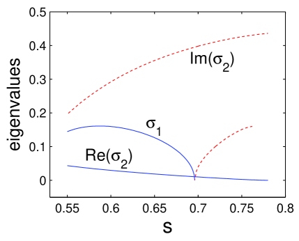
Figure 5: Eigenvalue spectrum of the 2nd family of vector solitons in the saturable model (4) at $\beta=0.16$. The solid (dashed) lines are the real (imaginary) parts of the eigenvalues.

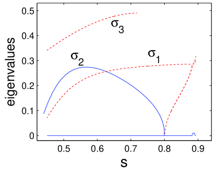
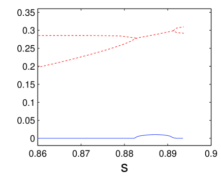
Figure 6: Eigenvalue spectrum of the 2nd family of vector solitons in the saturable model (4) at $\beta=0.49$. The solid (dashed) lines are the real (imaginary) parts of the eigenvalues. The right figure is a zoom-in of the left figure.

For the 2nd family, the eigenvalues $\lambda=\pm i\left[\beta_{1}(s)-\beta_{2}(s)\right]$ are embedded when $0.646<s<0.857$ and isolated when $s>0.857$. According to our prediction, the embedded eigenvalues should bifurcate to the complex unstable eigenvalues for $0<|\beta-\beta_{2}(s)|\ll 1$. However, it was claimed in [26] that vector solitons in the 2nd family were stable near the local bifurcation boundary $0<|\beta-\beta_{2}(s)|\ll 1$ for all values of $s$. In order to resolve this discrepancy, we have numerically determined the eigenvalue spectrum for vector solitons in the 2nd family by the shooting method. Figures 5 and 6 present numerical results for $\beta=0.16$ and $\beta=0.49$, respectively.

For $\beta=0.16$, the local bifurcation boundary of the 2nd family occurs at $s=0.785$ and the eigenvalues $\lambda=\pm i\left[\beta_{1}(s)-\beta_{2}(s)\right]$ are embedded, such that a pair of unstable complex eigenvalues $\lambda={\rm Re}(\sigma_{2})\pm i{\rm Im}(\sigma_{2})$ bifurcates for $s<0.785$. These complex eigenvalues indicate the oscillatory instability of vector solitons near the local bifurcation boundary $|\beta-\beta_{2}(s)|\ll 1$ for $\beta=0.16$. Thus the claim in [26] on the stability of 2nd-family vector solitons anywhere near the local bifurcation boundary is incorrect. Note that the complex eigenvalues $\lambda={\rm Re}(\sigma_{2})\pm i{\rm Im}(\sigma_{2})$ persist throughout the entire existence domain of the 2nd family, which is $0.513<s<0.785$ at $\beta=0.16$.

Furthermore, a pair of purely imaginary eigenvalues $\lambda=\pm i|\sigma_{1}|$ bifurcate from the end points $\lambda=\pm i\beta$ of the continuous spectrum at $s=0.763$, merge into the origin at $s=0.696$, and then bifurcate into a pair of real eigenvalues $\lambda=\pm\sigma_{1}$ for $s<0.696$. This exponential instability induced by the real eigenvalue $\lambda=\sigma_{1}$ has been reported in [26]. Since it was claimed in [26] that $z({\cal U})=0$ in the entire existence domain of the 2nd family of vector solitons, we conclude that the instability bifurcation at $s=0.696$ falls into the scenario of Appendix A.1 with $z({\cal L}_{1})=2$. In the interval $0.513<s<0.696$, the oscillatory instability is overshadowed by the exponential instability from the eigenvalue $\lambda=\sigma_{1}$. However, in the interval $0.696<s<0.785$, this oscillatory instability is the only instability experienced by vector solitons. Since ${\rm Re}(\sigma_{2})$ is less than $0.011$ in the interval $0.696<s<0.785$, it may explain why this oscillatory instability was missed in the numerical results of [26].

For $\beta=0.49$, the local bifurcation boundary of the 2nd family occurs at $s=0.894$, and the eigenvalues $\lambda=\pm i\left[\beta_{1}(s)-\beta_{2}(s)\right]$ are isolated, such that vector solitons near the local bifurcation boundary are spectrally stable. This is indeed confirmed in Fig. 6, where the spectrum diagram is displayed for all values of $s$. It is seen that at the local bifurcation boundary $s=0.894$, there are two pairs of isolated imaginary eigenvalues. The pair $\lambda=\pm i\left[\beta_{1}(s)-\beta_{2}(s)\right]=\pm 0.292i$ has the negative energy, while the pair $\lambda=\pm 0.310i$ has the positive energy. The second pair corresponds to the positive eigenvalue of ${\cal L}_{s}$ in (4.9). As $s$ moves leftward from the boundary point 0.894, these two imaginary eigenvalues move toward each other. At $s=0.891$, they coalesce and create a quadruple of complex eigenvalues, in agreement with Appendix A.3. However, this instability persists only in a tiny interval $0.882<s<0.891$, and it is very weak, with growth rates below 0.01. At $s=0.882$, these complex eigenvalues coalesce and bifurcate back into two pairs of purely imaginary eigenvalues again. When $s$ decreases further, one pair of these imaginary eigenvalues (denoted as $\pm\sigma_{1}$ in Fig. 6) always remain imaginary, but the other pair of imaginary eigenvalues ($\pm\sigma_{2}$ in Fig. 6) move toward zero and become real for $s<0.80$, in agreement with Appendix A.1. There is one more eigenvalue ($\sigma_{3}$) in Fig. 6, which bifurcates from the edge of the continuous spectrum at $s=0.718$, and always stays imaginary. The pattern of Fig. 6 differs from that of Fig. 5 in that complex instability is not set in at the local bifurcation boundary $\beta=\beta_{2}(s)$, and, once it is set in, it is confined in a narrow interval of $s$. Similar to the $\beta=0.16$ case above, this narrow interval of oscillatory instability was missed in [26], but the exponential instability was captured there.

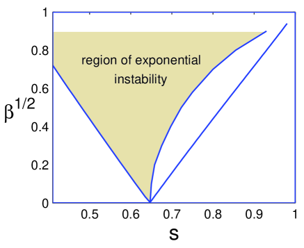
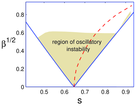
Figure 7: Regions (shaded) of exponential and oscillatory instabilities of the 2nd family of vector solitons in the saturable model (4).

Finally, we have mapped out the regions of exponential and oscillatory instabilities in the entire domain of existence for the 2nd family of vector solitons. The results are shown in Fig. 7. The almost-straight boundary lines show the local and nonlocal bifurcation boundaries [9]. The large domain of exponential instability away from the local bifurcation boundary corresponds to the one computed in Fig. 2 of [26]. The domain of oscillatory instability consists of two sub-domains. The larger sub-domain is at $s<0.857$, where the eigenvalues $\lambda=\pm i\left[\beta_{1}(s)-\beta_{2}(s)\right]$ at the local bifurcation boundary $\beta=\beta_{2}(s)$ are embedded. The smaller sub-domain is at $s>0.857$, where the eigenvalues $\lambda=\pm i\left[\beta_{1}(s)-\beta_{2}(s)\right]$ are isolated but bifurcate to complex eigenvalues away from the local bifurcation boundary $\beta=\beta_{2}(s)$. Both sub-domains of oscillatory instabily were missed in [26].

5 Summary

We have applied the Closure Theorem for the negative index of the linearized Hamiltonian to multi-hump vector solitons in the general coupled NLS equations (2.1). Unstable eigenvalues of the linearized problem (2.4) are approximated with the perturbation series expansions and found numerically with the shooting method. Not only the numerical results are in excellent agreement with the closure relation (2.9), but also the closure relation (2.9) shows that all unstable eigenvalues are recovered with the numerical shooting method. These analytical and numerical results establish that all multi-hump vector solitons in the non-integrable coupled cubic NLS equations are linearly unstable, while multi-hump vector solitons in the coupled saturable NLS equations can be linearly stable in certain regions of the parameter space. In the latter case, we have also discovered a new oscillatory instability which was missed before. This oscillatory instability significantly reduces the stability domains of vector solitons.

We note that the Closure Theorem is applied differently in Sections 3 and 4. For coupled cubic NLS equations, we compute the closure relation (2.9) from the right-hand side $n({\cal L}_{1})-p({\cal U})+n({\cal L}_{0})$ at the local bifurcation boundary and then match it with the number of unstable eigenvalues of the linearized problem (2.4). For coupled saturable NLS equations, we compute the closure relation (2.9) directly from the left-hand side $N_{\rm real}+2N_{\rm comp}+2N_{\rm imag}^{-}$ at the local bifurcation boundary and continue it in the entire existence domain.

While the negative index theory is well understood in [27] and well illustrated in [18, 17] and this paper, the following problem still remains a challenge: how do we understand the stability of vector solitons in sign-indefinite coupled-mode equations, such as the nonlinear Dirac equations? The Closure Theorem is obviously invalid for the Dirac equations as the continuous spectrum has both positive and negative energies. Thus a generalization of the Closure Theorem to such systems is highly desirable for future advances.

Acknowledgements. The work of D.E.P. was supported in part by NSERC grant No. 5-36694. The work of J.Y. was supported in part by NASA EPSCoR and AFOSR grants.

Appendix A Appendix: Bifurcations of unstable eigenvalues

Here we classify the four special cases, when one of the assumptions (i)–(iv) of the Closure Theorem fails. We derive sufficient conditions, when new unstable eigenvalues with ${\rm Re}(\lambda)>0$ bifurcate in the linearized problem (2.4) from eigenvalues with ${\rm Re}(\lambda)=0$. For clarity of notations, we use an equivalent form of the spectral problem (2.4):

$${\cal L}_{1}{\bf u}=\gamma{\cal L}_{0}^{-1}{\bf u},\qquad{\bf u}\in X_{c}^{(u)}(\mathbb{R}),$$ (A.1)

where $\gamma=-\lambda^{2}$ and $X_{c}^{(u)}(\mathbb{R})$ is the constrained subspace of $L^{2}(\mathbb{R})$:

$$X_{c}^{(u)}=\left\{{\bf u}\in L^{2}:\;\langle\Phi_{n}{\bf e}_{n},{\bf u}\rangle=0,\;n=1,...,N\right\}.$$ (A.2)

Here ${\bf e}_{1}$,…,${\bf e}_{N}$ are unit vectors in $\mathbb{R}^{N}$ and none of the components $\Phi_{n}(x)$ is assumed to vanish identically on $x\in\mathbb{R}$. Operator ${\cal L}_{0}$ is always invertible in $X_{c}^{(u)}(\mathbb{R})$, since eigenvectors $\{\Phi_{n}(x){\bf e}_{n}\}_{n=1}^{N}$ form a basis in the kernel of ${\cal L}_{0}$. In the domain ${\cal D}_{\epsilon}=\left\{\lambda\in\mathbb{C}:\;|\lambda|>\epsilon\right\}$ for any $\epsilon>0$, there exists a relation between ${\bf u}(x)$ and ${\bf w}(x)$:

$${\bf w}=\lambda{\cal L}_{0}^{-1}{\bf u},\qquad\lambda\in{\cal D}_{\epsilon},$$ (A.3)

such that two eigenvectors $({\bf u},{\bf w})^{T}$ and $({\bf u},-{\bf w})^{T}$ of the linearized problem (2.4) for $\lambda$ and $(-\lambda)$ correspond to a single eigenvector ${\bf u}(x)$ of the problem (A.1) for $\gamma=-\lambda^{2}$.

A.1 Zero eigenvalues of ${\cal L}_{1}$ and ${\cal L}_{0}$

The kernel of ${\cal L}_{0}$ has a basis of $N$ eigenvectors $\{\Phi_{n}(x){\bf e}_{n}\}_{n=1}^{N}$. Therefore, the existence domain of the vector solitons (2.2) is confined by the boundaries, where $\Phi_{n}(x)\equiv 0$ for some $n=1,...,N$. Let ${\cal B}$ be an open simply-connected domain in the parameter space $(\beta_{1},...,\beta_{N})$, where the vector solitons (2.2) exist. No bifurcations of zero eigenvalues of ${\cal L}_{0}$ occur in $\mbox{\boldmath$\beta$}\in{\cal B}$.

The kernel of ${\cal L}_{1}$ has always the eigenvector ${\bf\Phi}^{\prime}(x)$. When $z({\cal L}_{1})=1$, this is the only eigenvector in the kernel of ${\cal L}_{1}$. When $z({\cal L}_{1})>1$, additional linearly independent eigenvectors ${\bf u}_{0}(x)$ exist in the kernel of ${\cal L}_{1}$, such that the geometric multiplicity of $\lambda=0$ in the linearization problem (2.4) exceeds $(N+1)$. Under parameter continuation, the zero eigenvalue $\lambda=0$ generally moves either to the real or purely imaginary axes of $\lambda$. We study this bifurcation in the case, when $z({\cal L}_{1})=2$, $z({\cal U})=0$, and $\mbox{\boldmath$\beta$}\in{\cal B}$.

Proposition A.1

Let $\epsilon$ be the bifurcation parameter and, at $\epsilon=0$, there exists a non-zero eigenvector ${\bf u}_{0}\in X_{c}^{(u)}(\mathbb{R})$, such that ${\cal L}_{1}{\bf u}_{0}={\bf 0}$ and ${\bf u}_{0}$ is linearly independent of ${\bf\Phi}^{\prime}(x)$. Assume that ${\cal L}_{1}(\epsilon)$ and ${\cal L}_{0}(\epsilon)$ are $C^{1}$-functions at $\epsilon=0$, such that $l_{0}=\langle{\bf u}_{0},{\cal L}_{0}^{-1}(0){\bf u}_{0}\rangle\neq 0$ and $\delta l_{1}=\langle{\bf u}_{0},{\cal L}_{1}^{\prime}(0){\bf u}_{0}\rangle\neq 0$. Then, there exists $\epsilon_{0}>0$ such that the linearized problem (2.4) has a real positive eigenvalue $\lambda$ in the domain:

$${\cal D}_{\epsilon}=\left\{\epsilon:0<|\epsilon|<\epsilon_{0},\quad{\rm sign}(\epsilon)=-{\rm sign}(l_{0}\delta l_{1})\right\}.$$

• Proof. We expand solutions of (A.1) in power series of $\epsilon$:

  $${\bf u}(x)={\bf u}_{0}(x)+\epsilon{\bf u}_{1}(x)+{\rm O}(\epsilon^{2}),\qquad\gamma=\epsilon\gamma_{1}+{\rm O}(\epsilon^{2}).$$ (A.4)

  The function ${\bf u}_{1}(x)$ solves the non-homogeneous problem in $X_{c}^{(u)}({\mathbb{R}})$:

  $${\cal L}_{1}(0){\bf u}_{1}+{\cal L}_{1}^{\prime}(0){\bf u}_{0}=\gamma_{1}{\cal L}_{0}^{-1}(0){\bf u}_{0}.$$ (A.5)

  Using the Fredholm Alternative Theorem, we find from (A.5) that $\delta l_{1}=\gamma_{1}l_{0}$. If $\delta l_{1}\neq 0$, $l_{0}\neq 0$, and ${\rm sign}(\epsilon)=-{\rm sign}(l_{0}\delta l_{1})$, the eigenvalue $\gamma$ is negative in the first order of $\epsilon$, such that $\lambda=\pm\sqrt{-\gamma}$ are real.  

Corollary A.1

Let ${\cal L}_{0}$ be positive definite, such that $l_{0}>0$. A new negative eigenvalue $\mu(\epsilon)$ of ${\cal L}_{1}$ as $\epsilon\neq 0$ results in a new negative eigenvalue $\gamma(\epsilon)$ of the problem (A.1), such that

$$\lim_{\epsilon\to 0}\frac{\gamma}{\mu}=\frac{\langle{\bf u}_{0},{\bf u}_{0}\rangle}{\langle{\bf u}_{0},{\cal L}_{0}^{-1}(0){\bf u}_{0}\rangle}.$$ (A.6)

Bifurcation $z({\cal L}_{1})>1$ may occur only if $N>1$ in the system (2.1). Analysis of this bifurcation with the Lyapunov-Schmidt reduction method are reported in a similar content in [17, 18, 30].

A.2 Zero eigenvalues of ${\cal U}$

When $z({\cal U})>0$, algebraic multiplicity of $\lambda=0$ exceeds $(2N+2)$. Under a parameter continuation, the zero eigenvalue $\lambda=0$ generally moves either to the real or purely imaginary axis of $\lambda$. We study this bifurcation in the case, when $z({\cal U})=1$, $z({\cal L}_{1})=1$, and $\mbox{\boldmath$\beta$}\in{\cal B}$.

Proposition A.2

Let $\epsilon$ be the bifurcation parameter and, at $\epsilon=0$, there exists a non-zero eigenvector $\mbox{\boldmath$\nu$}\in\mathbb{R}^{N}$, ${\cal U}\mbox{\boldmath$\nu$}={\bf 0}$, such that the eigenvector ${\bf u}_{0}\in X_{c}^{(u)}(\mathbb{R})$ solves the problem:

$${\cal L}_{1}{\bf u}_{0}=-\sum_{n=1}^{N}\nu_{n}\Phi_{n}(x){\bf e}_{n}.$$ (A.7)

Assume that ${\cal L}_{1}(\epsilon)$, ${\cal L}_{0}(\epsilon)$, and ${\cal U}(\epsilon)$ are $C^{1}$-functions at $\epsilon=0$, such that $l_{0}=\langle{\bf u}_{0},{\cal L}_{0}^{-1}(0){\bf u}_{0}\rangle\neq 0$ and $\delta u=\langle\mbox{\boldmath$\nu$},{\cal U}^{\prime}(0)\mbox{\boldmath$\nu$}\rangle\neq 0$. Then, there exists $\epsilon_{0}>0$ such that the linearized problem (2.4) has a real positive eigenvalue $\lambda$ in the domain:

$${\cal D}_{\epsilon}=\left\{\epsilon:0<|\epsilon|<\epsilon_{0},\quad{\rm sign}(\epsilon)=-{\rm sign}(l_{0}\delta u)\right\}.$$

• Proof. If there exists $\mbox{\boldmath$\nu$}\in\mathbb{R}^{N}$, such that ${\cal U}(0)\mbox{\boldmath$\nu$}={\bf 0}$, then the eigenvector ${\bf u}_{0}(x)$ for the problem (A.7) is given explicitly as

  $${\bf u}_{0}(x)=\sum_{n=1}^{N}\nu_{n}\frac{\partial{\bf\Phi}(x)}{\partial\beta_{n}}.$$ (A.8)

  Using ${\cal L}_{1}\partial{\bf\Phi}/\partial\beta_{n}=-\Phi_{n}{\bf e}_{n}$ and ${\cal L}_{0}\Phi_{n}{\bf e}_{n}={\bf 0}$ for any $\epsilon$, we obtain the following derivative relations:

  $${\cal L}_{1}(0)\frac{\partial\mbox{\boldmath$\Phi$}^{\prime}(0)}{\partial\beta_{n}}+{\cal L}_{1}^{\prime}(0)\frac{\partial\mbox{\boldmath$\Phi$}}{\partial\beta_{n}} = -\Phi_{n}^{\prime}(0){\bf e}_{n},$$ (A.9)

  $${\cal L}_{0}(0)\Phi_{n}^{\prime}(0){\bf e}_{n}+{\cal L}_{0}^{\prime}(0)\Phi_{n}{\bf e}_{n} = 0,$$ (A.10)

  where ${\bf\Phi}^{\prime}(0)$ stands for derivative of ${\bf\Phi}(\epsilon)$ in $\epsilon$. We expand solutions of (A.1) in power series of $\epsilon$:

  $${\bf u}(x)={\bf u}_{0}(x)+\epsilon{\bf u}_{1}(x)+{\rm O}(\epsilon^{2}),\qquad\gamma=\epsilon\gamma_{1}+{\rm O}(\epsilon^{2}).$$ (A.11)

  Since the eigenvector ${\bf u}_{0}(x)$ solves the non-homogeneous problem (A.7), the relation between ${\bf u}(x)$ and ${\bf w}(x)$ is modified as follows:

  $${\bf w}=\lambda{\cal L}_{0}^{-1}{\bf u}+\frac{1}{\lambda}\sum_{n=1}^{N}\nu_{n}\Phi_{n}(x){\bf e}_{n}.$$ (A.12)

  As a result, the function ${\bf u}_{1}(x)$ solves the non-homogeneous problem:

  $${\cal L}_{1}(0){\bf u}_{1}+{\cal L}_{1}^{\prime}(0){\bf u}_{0}=\gamma_{1}{\cal L}_{0}^{-1}(0){\bf u}_{0}-\sum_{n=1}^{N}\nu_{n}\Phi_{n}^{\prime}(0){\bf e}_{n},$$ (A.13)

  subject to the constraints:

  $$\langle\Phi_{n}(0){\bf e}_{n},{\bf u}_{1}\rangle+\langle\Phi_{n}^{\prime}(0){\bf e}_{n},{\bf u}_{0}\rangle=0.$$ (A.14)

  Using the Fredholm Alternative Theorem, we find from (A.13) and (A.14) that

  $$\langle{\bf u}_{0},{\cal L}_{1}^{\prime}(0){\bf u}_{0}\rangle=\gamma_{1}\langle{\bf u}_{0},{\cal L}_{0}^{-1}(0){\bf u}_{0}\rangle-2\sum_{n=1}^{N}\nu_{n}\langle\Phi_{n}^{\prime}(0){\bf e}_{n},{\bf u}_{0}\rangle.$$ (A.15)

  As a result,

  $$\gamma_{1}\langle{\bf u}_{0}|{\cal L}_{0}^{-1}(0){\bf u}_{0}\rangle=\sum_{n=1}^{N}\sum_{m=1}^{N}\nu_{n}\nu_{m}\frac{\partial}{\partial\epsilon}\langle\Phi_{m}(\epsilon){\bf e}_{m},\frac{\partial{\bf\Phi}(\epsilon)}{\partial\beta_{n}}\rangle\biggr{|}_{\epsilon=0}=\frac{1}{2}\langle\mbox{\boldmath$\nu$},{\cal U}^{\prime}(0)\mbox{\boldmath$\nu$}\rangle,$$ (A.16)

  such that $\delta u=2\gamma_{1}l_{0}$. When $\delta u\neq 0$, $l_{0}\neq 0$, and ${\rm sign}(\epsilon)=-{\rm sign}(l_{0}\delta u)$, the eigenvalue $\gamma$ is negative in the first order of $\epsilon$, such that $\lambda=\pm\sqrt{-\gamma}$ are real.  

Corollary A.2

Let ${\cal L}_{0}$ be positive definite, such that $l_{0}>0$. A new negative eigenvalue $\mu(\epsilon)$ of ${\cal U}$ as $\epsilon\neq 0$ results in a new negative eigenvalue $\gamma(\epsilon)$ of the problem (A.1).

Bifurcation $z({\cal U})>0$ was analyzed in [28, 31] with power series expansions of the problem (2.4) near $\lambda=0$ and in [5, 19] with Taylor series expansions of the Evans function.

A.3 Multiple non-zero eigenvalues of zero energy

When the problem (2.4) has a multiple eigenvalue $\lambda=\lambda_{0}\in i\mathbb{R}$ of zero energy, the corresponding eigenvector $({\bf u}_{0},{\bf w}_{0})^{T}$ satisfies the conditions of the Fredholm Alternative Theorem: $\langle{\bf u}_{0},{\cal L}_{1}{\bf u}_{0}\rangle=0$, $\langle{\bf w}_{0},{\cal L}_{0}{\bf w}_{0}\rangle=0$, such that $h[{\bf u}_{0},{\bf w}_{0}]=0$ and $l_{0}=\langle{\bf u}_{0},{\cal L}_{0}^{-1}{\bf u}_{0}\rangle=0$. Under parameter continuations, multiple eigenvalues are generally destroyed and new complex eigenvalues $\lambda$ may arise in the problem (2.4). We study this bifurcation in the case, when a multiple eigenvalue $\lambda=\lambda_{0}$ has algebraic multiplicity two and geometric multiplicity one, while $\mbox{\boldmath$\beta$}\in{\cal B}\cup\partial{\cal B}$.

Proposition A.3

Let $\epsilon$ be the bifurcation parameter and, at $\epsilon=0$, there exist non-zero eigenvectors ${\bf u}_{0},{\bf u}_{0}^{\prime}\in X_{c}^{(u)}(\mathbb{R})$ for $\gamma_{0}\in\mathbb{R}$ and $\gamma_{0}<\beta_{\rm min}^{2}$, such that

$${\cal L}_{1}{\bf u}_{0} = \gamma_{0}{\cal L}_{0}^{-1}{\bf u}_{0},$$ (A.17)

$${\cal L}_{1}{\bf u}_{0}^{\prime} = \gamma_{0}{\cal L}_{0}^{-1}{\bf u}_{0}^{\prime}+{\cal L}_{0}^{-1}{\bf u}_{0},$$ (A.18)

and $l_{0}=\langle{\bf u}_{0},{\cal L}_{0}^{-1}{\bf u}_{0}\rangle=0$. Assume that ${\cal L}_{1}(\epsilon)$ and ${\cal L}_{0}(\epsilon)$ are $C^{1}$-functions at $\epsilon=0$, such that $l_{0}^{\prime}=\langle{\bf u}_{0},{\cal L}_{0}^{-1}(0){\bf u}_{0}^{\prime}\rangle\neq 0$ and $\delta h=\langle{\bf u}_{0},\left({\cal L}_{1}^{\prime}(0)-\gamma_{0}{\cal L}_{0}^{-1\prime}(0)\right){\bf u}_{0}\rangle\neq 0$. Then, there exists $\epsilon_{0}>0$ such that the linearized problem (2.4) has two complex eigenvalues $\lambda$ with ${\rm Re}(\lambda)>0$ in the domain:

$${\cal D}_{\epsilon}=\left\{\epsilon:0<|\epsilon|<\epsilon_{0},\quad{\rm sign}(\epsilon)=-{\rm sign}(l_{0}^{\prime}\delta h)\right\}.$$

• Proof. We expand solutions of (A.1) in power series of $\epsilon^{1/2}$:

  $${\bf u}(x) = {\bf u}_{0}(x)+\epsilon^{1/2}\gamma_{1}{\bf u}_{0}^{\prime}(x)+\epsilon{\bf u}_{2}(x)+{\rm O}(\epsilon^{3/2}),$$ (A.19)

  $$\gamma = \gamma_{0}+\epsilon^{1/2}\gamma_{1}+\epsilon\gamma_{2}+{\rm O}(\epsilon^{3/2}).$$ (A.20)

  The function ${\bf u}_{2}(x)$ solves the non-homogeneous problem in $X_{c}^{(u)}(\mathbb{R})$:

  $${\cal L}_{1}(0){\bf u}_{2}+{\cal L}_{1}^{\prime}(0){\bf u}_{0}=\gamma_{0}{\cal L}_{0}^{-1}(0){\bf u}_{2}+\gamma_{0}{\cal L}_{0}^{-1\prime}(0){\bf u}_{0}+\gamma_{1}^{2}{\cal L}_{0}^{-1}(0){\bf u}_{0}^{\prime}+\gamma_{2}{\cal L}_{0}^{-1}(0){\bf u}_{0}.$$ (A.21)

  Using the Fredholm Alternative Theorem, we find from (A.21) that $\delta h=\gamma_{1}^{2}l_{0}^{\prime}$. Since $(\gamma-\gamma_{0})^{2}=\epsilon\gamma_{1}^{2}+{\rm O}(\epsilon^{3/2})$, the eigenvalues $\gamma$ bifurcate into the complex plane if $l_{0}^{\prime}\neq 0$, $\delta h\neq 0$, and ${\rm sign}(\epsilon)=-{\rm sign}(l_{0}^{\prime}\delta h)$.  

Corollary A.3

Let $l_{0}^{\prime}\neq 0$ and $\delta h\neq 0$. There exists $\epsilon_{0}>0$ such that the problem (A.1) has two real eigenvalues $\gamma$ in the domain,

$${\cal D}_{\epsilon}=\left\{\epsilon:0<|\epsilon|<\epsilon_{0},\quad{\rm sign}(\epsilon)={\rm sign}(l_{0}^{\prime}\delta h)\right\}$$

with oppositely signed quadratic forms

$$\langle{\bf u},{\cal L}_{0}^{-1}{\bf u}\rangle=2\epsilon^{1/2}\gamma_{1}l_{0}^{\prime}+{\rm O}(\epsilon).$$

When $0<\gamma_{0}<\beta_{\rm min}$, multiple eigenvalue $\lambda=\lambda_{0}$ is purely imaginary, and the bifurcation of Proposition A.3 is the instability bifurcation. When $\gamma_{0}<0$, the eigenvalue $\lambda=\lambda_{0}$ is purely real and is thus already unstable. Characteristic features of bifurcation of multiple eigenvalues were analyzed in [12]. This bifurcation is generic when purely imaginary eigenvalues of positive and negative energies $h[{\bf u},{\bf w}]$ coalesce, according to Corollary A.3 [32]. General results on the collisions of purely imaginary eigenvalues of different energies and the concept of so-called Krein signatures can be found in [22].

A.4 Embedded eigenvalues

When the problem (2.4) has an embedded eigenvalue $\lambda=\lambda_{0}\in i\mathbb{R}$ with $|{\rm Im}(\lambda_{0})|>\beta_{\rm min}$, it is generically unstable under parameter continuation [12, 20, 21]. When it has a positive energy, it disappears from the continuous spectrum, while when it has a negative energy, it bifurcates as complex unstable eigenvalues with ${\mathop{\mathrm{Re}}}(\lambda)>0$ [8]. We study this bifurcation in the case, when an embedded eigenvalue has the geometric and algebraic multiplicities one, while $\mbox{\boldmath$\beta$}\in{\cal B}\cup\partial{\cal B}$.

Proposition A.4

Let $\epsilon$ be the bifurcation parameter and, at $\epsilon=0$, there exist a non-zero eigenvector ${\bf u}_{0}\in X_{c}^{(u)}(\mathbb{R})$ for $\gamma_{0}\in\mathbb{R}$, $\gamma_{0}>\beta_{\rm min}^{2}$, such that

$${\cal L}_{1}{\bf u}_{0}=\gamma_{0}{\cal L}_{0}^{-1}{\bf u}_{0}.$$ (A.22)

Assume that ${\cal L}_{1}(\epsilon)$ and ${\cal L}_{0}(\epsilon)$ are $C^{1}$-functions at $\epsilon=0$, such that $l_{0}=\langle{\bf u}_{0},{\cal L}_{0}^{-1}(0){\bf u}_{0}\rangle<0$ and $\Gamma\neq 0$ in (A.29) below. Then, there exists $\epsilon_{0}>0$ such that the linearized problem (2.4) has two complex eigenvalues $\lambda$ with ${\rm Re}(\lambda)>0$.

• Proof. For embedded eigenvalues, we use the linearized problem in the original form (2.4). Consider perturbation series expansions near the embedded eigenvalue $\lambda=\lambda_{0}$, with ${\rm Im}(\lambda_{0})>\beta_{\rm min}$:

  $${\bf u}(x) = {\bf u}_{0}(x)+\epsilon{\bf u}_{1}(x)+\epsilon^{2}{\bf u}_{2}(x)+{\rm O}(\epsilon^{3}),$$ (A.23)

  $${\bf w}(x) = {\bf w}_{0}(x)+\epsilon{\bf w}_{1}(x)+\epsilon^{2}{\bf w}_{2}(x)+{\rm O}(\epsilon^{3}),$$ (A.24)

  and

  $$\lambda=\lambda_{0}+\epsilon\lambda_{1}+\epsilon^{2}\lambda_{2}+{\rm O}(\epsilon^{3}).$$ (A.25)

  Corrections of the perturbation series (A.23) and (A.24) satisfy linear non-homogeneous equations following from the linearized problem (2.4):

  $${\cal L}_{1}(0){\bf u}_{1}+\lambda_{0}{\bf w}_{1} = -{\cal L}_{1}^{\prime}(0){\bf u}_{0}-\lambda_{1}{\bf w}_{0},$$

  $${\cal L}_{0}(0){\bf w}_{1}-\lambda_{0}{\bf u}_{1} = -{\cal L}_{0}^{\prime}(0){\bf w}_{0}+\lambda_{1}{\bf u}_{0}$$ (A.26)

  and

  $${\cal L}_{1}(0){\bf u}_{2}+\lambda_{0}{\bf w}_{2} = -{\cal L}_{1}^{\prime}(0){\bf u}_{1}-\frac{1}{2}{\cal L}_{1}^{\prime\prime}(0){\bf u}_{0}-\lambda_{1}{\bf w}_{1}-\lambda_{2}{\bf w}_{0},$$

  $${\cal L}_{0}(0){\bf w}_{2}-\lambda_{0}{\bf u}_{2} = -{\cal L}_{0}^{\prime}(0){\bf w}_{1}-\frac{1}{2}{\cal L}_{0}^{\prime\prime}(0){\bf w}_{0}+\lambda_{1}{\bf u}_{1}+\lambda_{2}{\bf u}_{0}.$$ (A.27)

  Bounded solutions of the problem (A.26) exist only if the right-hand-side is orthogonal to the eigenvector $({\bf u}_{0},{\bf w}_{0})$. The solvability condition results in the equation:

  $$\lambda_{1}\left(\langle{\bf w}_{0},{\bf u}_{0}\rangle-\langle{\bf u}_{0},{\bf w}_{0}\rangle\right)=\langle{\bf u}_{0},{\cal L}_{1}^{\prime}(0){\bf u}_{0}\rangle+\langle{\bf w}_{0},{\cal L}_{0}^{\prime}(0){\bf w}_{0}\rangle,$$

  such that ${\rm Re}(\lambda_{1})=0$. Since the eigenvalue $\lambda=\lambda_{0}$ belongs to the continuous spectrum of the problem (2.4), the correction terms $({\bf u}_{1},{\bf w}_{1})$ have non-vanishing tails in the limit $|x|\to\infty$. Assuming that $\beta_{1}\leq\beta_{2}\leq...\leq\beta_{N}$, we add Sommerfeld radiation conditions to uniquely determine the correction terms $({\bf u}_{1},{\bf w}_{1})$:

  $$\left(\begin{array}[]{c}{\bf u}_{1}\\ {\bf w}_{1}\end{array}\right)\rightarrow\sum_{j=1}^{K_{\lambda_{0}}}g_{j}^{\pm}\left(\begin{array}[]{cc}{\bf e}_{j}\\ i{\bf e}_{j}\end{array}\right)e^{\mp ik_{j}x},\qquad x\to\pm\infty,$$ (A.28)

  where $g_{j}^{\pm}$ are some constants, $k_{j}=\sqrt{({\rm Im}(\lambda_{0})-\beta_{j})/d_{j}}$, and $K_{\lambda_{0}}$ is the number of branches with $k_{j}\in\mathbb{R}$. It follows from (A.26) that

  $${\rm Im}\left(\langle{\bf u}_{1},{\cal L}_{1}^{\prime}(0){\bf u}_{0}\rangle+\langle{\bf w}_{1},{\cal L}_{0}^{\prime}(0){\bf w}_{0}\rangle+\lambda_{1}\langle{\bf u}_{1},{\bf w}_{0}\rangle-\lambda_{1}\langle{\bf w}_{1},{\bf u}_{0}\rangle\right)$$ (A.29)

  $$= -\frac{1}{2i}\left(\langle{\bf u}_{1},{\cal L}_{1}{\bf u}_{1}\rangle+\langle{\bf w}_{1},{\cal L}_{0}{\bf w}_{1}\rangle-\langle{\cal L}_{1}{\bf u}_{1},{\bf u}_{1}\rangle-\langle{\cal L}_{0}{\bf w}_{1},{\bf w}_{1}\rangle\right)$$

  $$= -2\sum_{j=1}^{K_{\lambda_{0}}}d_{j}k_{j}\left(|g^{+}_{j}|^{2}+|g^{-}_{j}|^{2}\right)\equiv\Gamma\leq 0.$$

  Again, bounded solutions of the problem (A.27) exist only if

  $$\lambda_{2}\left(\langle{\bf w}_{0},{\bf u}_{0}\rangle-\langle{\bf u}_{0},{\bf w}_{0}\rangle\right)+\lambda_{1}\left(\langle{\bf w}_{0},{\bf u}_{1}\rangle-\langle{\bf u}_{0},{\bf w}_{1}\rangle\right)$$

  $$=\langle{\bf u}_{0},{\cal L}_{1}^{\prime}(0){\bf u}_{1}\rangle+\langle{\bf w}_{0},{\cal L}_{0}^{\prime}(0){\bf w}_{1}\rangle+\frac{1}{2}\langle{\bf u}_{0},{\cal L}_{1}^{\prime\prime}(0){\bf u}_{0}\rangle+\frac{1}{2}\langle{\bf w}_{0},{\cal L}_{0}^{\prime\prime}(0){\bf w}_{0}\rangle,$$ (A.30)

  such that

  $${\rm Re}(\lambda_{2})=\frac{{\rm Im}\left(\langle{\bf u}_{1},{\cal L}_{1}^{\prime}(0){\bf u}_{0}\rangle+\langle{\bf w}_{1},{\cal L}_{0}^{\prime}(0){\bf w}_{0}\rangle\right)}{2{\rm Im}(\lambda_{0})\langle{\bf u}_{0},{\cal L}_{0}^{-1}{\bf u}_{0}\rangle}=-\sum_{j=1}^{K_{\lambda_{0}}}\frac{d_{j}k_{j}\left(|g_{j}^{+}|^{2}+|g_{j}^{-}|^{2}\right)}{{\rm Im}(\lambda_{0})\langle{\bf u}_{0},{\cal L}_{0}^{-1}{\bf u}_{0}\rangle}.$$ (A.31)

  When $\Gamma\neq 0$ and $l_{0}=\langle{\bf u}_{0},{\cal L}_{0}^{-1}(0){\bf u}_{0}\rangle<0$, the embedded eigenvalue $\lambda=\lambda_{0}$ becomes a complex unstable eigenvalue $\lambda$ with ${\rm Re}(\lambda)>0$.  

Corollary A.4

The linearized problem (2.4) does not have complex or embedded eigenvalues $\lambda$ if $l_{0}=\langle{\bf u}_{0},{\cal L}_{0}^{-1}(0){\bf u}_{0}\rangle>0$ and $\Gamma\neq 0$.

• Proof. The formal computation in (A.31) predicts that ${\rm Re}(\lambda_{2})<0$, when $\Gamma\neq 0$ and $l_{0}>0$. However, the correction terms $({\bf u}_{1},{\bf w}_{1})^{T}$ in (A.28) grow exponentially in $x$, since $k_{j}(\lambda)=\sqrt{({\rm Im}(\lambda)-i{\rm Re}(\lambda)-\beta_{j})/d_{j}}$ implies that ${\rm Im}(k_{j})>0$. The embedded eigenvalue $\lambda=\lambda_{0}$ becomes a resonant pole with ${\rm Re}(\lambda)<0$.  

Characteristic features of bifurcations of embedded eigenvalues were analyzed in [8, 12]. This bifurcation is generic for multi-hump vector solitons at the boundaries of the existence domain $\mbox{\boldmath$\beta$}\in\partial{\cal B}$ [35].

Summarizing, there exist four bifurcations, which may lead to unstable eigenvalues in the spectral problem (2.4): (i) $z({\cal L}_{1})>1$, (ii) $z({\cal U})>0$, (iii) multiple eigenvalue $\lambda_{0}\in i\mathbb{R}$, $|{\rm Im}(\lambda_{0})|<\beta_{\rm min}$, and (iv) embedded eigenvalue $\lambda_{0}\in i\mathbb{R}$, $|{\rm Im}(\lambda_{0})|>\beta_{\rm min}$. Let $n_{X}(h)$ be the negative index of the linearized Hamiltonian in the constrained space $X_{c}^{(u)}(\mathbb{R})$, i.e. the number of negative eigenvalues of ${\cal L}_{1}$ and ${\cal L}_{0}$ in $X_{c}^{(u)}(\mathbb{R})$. It is known from [13] (see also [27, 28]) that

$$n_{X}(h)=n({\cal L}_{1})-p({\cal U})+n({\cal L}_{0}).$$ (A.32)

The closure relation (2.9) gives then:

$$n_{X}(h)=N_{\rm real}+2N_{\rm imag}^{-}+2N_{\rm comp}.$$ (A.33)

It is clear from (A.33) that bifurcations (i) and (ii) change the negative index $n_{X}(h)$ due to a change in $N_{\rm real}$ by one, while bifurcations (iii) and (iv) do not change the negative index $n_{X}(h)$ due to an exchange in $N_{\rm imag}^{-}$ and $N_{\rm comp}$.

References

- [1] G.P. Agrawal, Nonlinear Fiber Optics (Academic Press, San Diego, 1989).
- [2] N.N. Akhmediev, A.V. Buryak, J.M. Soto-Crespo, and D.R. Andersen, “Phase-locked stationary soliton states in birefringent nonlinear optical fibers.” J. Opt. Soc. Am. B 12, 434 (1995).
- [3] N. Akhmediev and A. Ankiewicz, Solitons, Nonlinear Pulses and Beams (Chapman & Hall, London, 1997).
- [4] D.J. Benney and A.C. Newell, “The propagation of nonlinear wave envelops.” J. Math. Phys. 46, 133-139 (1967).
- [5] T.J. Bridges and G. Derks, “Unstable eigenvalues and the linearization about solitary waves and fronts with symmetry”, Proc. Roy. Soc. Lond. A 455, 2427–2469 (1999).
- [6] Z. Chen, M. Segev, T.H. Coskun and D.N. Christodoulides, “Observation of incoherently coupled photorefractive spatial soliton pairs.” Opt. Lett. 21, 1436-1438 (1996).
- [7] Z. Chen, M. Acks, E.A. Ostrovskaya and Y.S. Kivshar, “Observation of bound states of interacting vector solitons.” Opt. Lett. 25, 417-419 (2000).
- [8] S. Cuccagna, D. Pelinovsky, and V. Vougalter: ”Spectra of positive and negative energies in the linearized NLS problem”, Comm.Pure Appl.Math. 58, 1-29 (2004)
- [9] A.R. Champneys and J. Yang, ”A scalar nonlocal bifurcation of solitary waves for coupled nonlinear Schrödinger systems”, Nonlinearity 15, 2165–2192 (2002).
- [10] D.N. Christodoulides and R.I. Joseph, “Vector solitons in birefringent nonlinear dispersive media.” Opt. Lett. 13, 53-55 (1988).
- [11] D. N. Christodoulides, S. R. Singh, M. I. Carvalho, and M. Segev, “Incoherently coupled soliton pairs in biased photorefractive crystals”, Appl. Phys. Lett. 68, 1763-1765 (1996).
- [12] M. Grillakis, “Analysis of the linearization around a critical point of an infinite dimensional Hamiltonian system”, Comm. Pure Appl. Math. 43, 299–333 (1990).
- [13] M. Grillakis, J. Shatah, and W. Strauss, “Stability theory of solitary waves in the presence of symmetry. II”, J. Funct. Anal. 94, 308–348 (1990).
- [14] M. Haelterman and A.P. Sheppard, ”Bifurcation phenomena and multiple soliton-bound states in isotropic Kerr media”, Phys. Rev. E 49, 3376–3381 (1994).
- [15] A. Hasegawa and Y. Kodama, Solitons in optical communications. Clarendon, Oxford, 1995.
- [16] Yu. S. Kivshar and G.P. Agrawal, Optical Solitons: ¿From Fibers to Photonic Crystals (Academic Press, San Diego, 2003).
- [17] T. Kapitula and P. Kevrekidis, “Linear stability in perturbed Hamiltonian systems: the case study”, J. Phys. A: Math. Gen. 37, 7509-7526 (2004).
- [18] T. Kapitula, P. Kevrekidis, and B. Sandstede, “”Counting eigenvalues via the Krein signature in infinite-dimensional Hamiltonian systems”, Physica D 195, 263–282 (2004).
- [19] T. Kapitula and B. Sandstede, “Stability of bright solitary wave solutions to perturbed nonlinear Schrödinger equations”, Physica D 124, 58–103 (1998).
- [20] Y. Li and K. Promislow, “Structural stability of non-ground state traveling waves of coupled nonlinear Schrödinger equations”, Physica D 124, 137–165 (1998).
- [21] Y. Li and K. Promislow, “The mechanism of the polarizational mode instability in birefringent fiber optics”, SIAM J. Math. Anal. 31, 1351–1373 (2000).
- [22] R.S. MacKay, ”Stability of equilibria of Hamiltonian systems”, in ”Hamiltonian Dynamical Systems” (R.S. MacKay and J. Meiss, eds.) (Adam Hilger, 1987), 137–153.
- [23] C.R. Menyuk, “Nonlinear pulse propagation in birefringent optical fibers.” IEEE J. Quantum Electron, QE-23, 174 (1987).
- [24] M. Mitchell, M. Segev and D.N. Christodoulides, “Observation of multihump multimode solitons.” Phys. Rev. Lett. 80, 4657-4660 (1998).
- [25] E.A. Ostrovskaya and Yu.S. Kivshar, “Multi-hump optical solitons in a saturable medium”, J. Opt. B 1, 77–83 (1999).
- [26] E.A. Ostrovskaya, Yu.S. Kivshar, D.V. Skryabin, and W.J. Firth, “Stability of multihump optical solitons”, Phys. Rev. Lett. 83, 296–299 (1999).
- [27] D.E. Pelinovsky, “Inertia law for spectral stability of solitary waves in coupled nonlinear Schrödinger equations”, Proc. Roy. Soc. Lond. A, in print (2005).
- [28] D.E. Pelinovsky and Yu.S. Kivshar, “Stability criterion for multicomponent solitary waves”, Phys. Rev. E 62, 8668–8676 (2000).
- [29] D.E. Pelinovsky and J. Yang, “Internal oscillations and radiation damping of vector solitons”, Stud. Appl. Math. 105, 245–276 (2000).
- [30] B. Sandstede, “Stability of multiple-pulse solutions”, Trans. Am. Math. Soc. 350, 429–472 (1998).
- [31] D.V. Skryabin, “Stability of multi-parameter solitons: asymptotic approach”, Physica D 139, 186–193 (2000).
- [32] D.V. Skryabin, “Instabilities of vortices in a binary mixture of trapped Bose–Einstein condensates: role of collective excitations with positive and negative energies”, Phys. Rev. A 63, 013602 (2001).
- [33] A.W. Snyder, S.J. Hewlett and D.J. Mitchell, “Dynamic spatial solitons.” Phys. Rev. Lett. 72, 1012 (1994).
- [34] M.V. Tratnik and J.E. Sipe, “Bound solitary waves in a birefringent optical fiber.” Phys. Rev. A 38, 2011-2017 (1988).
- [35] T.P.Tsai and H.T.Yau, ”Stable directions for excited states of nonlinear Schrödinger equations”, Comm. Partial Diff. Eq. 27, 2363–2402 (2002)
- [36] J. Yang, “Classification of the solitary waves in coupled nonlinear Schrödinger equations”, Physica D 108, 92–112 (1997).
- [37] J. Yang, “Vector solitons and their internal oscillations in birefringent nonlinear optical fibers”, Stud. Appl. Math. 98, 61-97 (1997).
- [38] J. Yang, “Interactions of vector solitons”, Phys. Rev. E 64, 026607 (2001).
- [39] J. Yang, “Internal oscillations and instability characteristics of (2+1) dimensional solitons in a saturable nonlinear medium”, Phys. Rev. E. 66, 026601 (2002).
- [40] J. Yang, “A tail-matching method for the linear stability of multi-vector-soliton bound states”, AMS book series Contemporary Mathematics, editors D.P. Clemens and G. Tang (2004).
- [41] J. Yang and D.E. Pelinovsky, ”Stable vortex and dipole vector solitons in a saturable nonlinear medium”, Phys. Rev. E 67, 016608 (2003).