A tail-matching method for the linear stability of multi-vector-soliton bound states

Abstract

Linear stability of multi-vector-soliton bound states in the coupled nonlinear Schrödinger equations is analyzed using a new tail-matching method. Under the condition that individual vector solitons in the bound states are wave-and-daughter-waves and widely separated, small eigenvalues of these bound states that bifurcate from the zero eigenvalue of single vector solitons are calculated explicitly. It is found that unstable eigenvalues from phase-mode bifurcations always exist, thus the bound states are always linearly unstable. This tail-matching method is simple, but it gives identical results as the Karpman-Solev’ev-Gorshkov-Ostrovsky method.

Mathematics Subject Classification: 35Q55, 35Pxx, 74J35.

Key words: linear stability; coupled NLS equations; tail-matching method.

1 Introduction

Nonlinear optics and fiber communication systems are advancing very rapidly these days. In this process, a widely-used mathematical model is the coupled nonlinear Schrödinger (NLS) equations which govern pulse propagation in birefringent fibers [1, 2, 3]. Similar equations with a saturable nonlinearity also govern the interaction of two incoherently-coupled laser beams [4, 5]. These equations arise in water-wave interactions as well [6, 7]. Solution properties of the coupled NLS equations have been examined extensively in the past ten years. It is known that these equations admit single-hump vector solitons due to a nonlinear mutual trapping effect [8, 9]. When these solitons are perturbed, they undergo long-lived internal oscillations [10, 11, 12]. When they collide with each other, a fractal structure can arise in the parameter space [13, 14].

Multi-vector-soliton bound states also exist in the coupled NLS equations [15]. These states are pieced together by several single-hump vector solitons. They received much attention because of several reasons. First, in fiber communication systems, pulse-pulse interference impairs the system performance. If multi-soliton bound states exist, these solutions would have implications to system designs. Second, the existence of such bound states is noteworthy because they can not exist in the NLS equation [16]. Thirdly, these states are closely related to similar states in incoherent laser beams, which have been observed experimentally [17].

After the numerical discovery of these multi-vector-soliton bound states in [15], their analytical construction was made in [18] by a tail-matching technique. Their linear-stability problem was studied later in [21] by an extension of the Karpman-Solev’ev-Gorshkov-Ostrovsky (KSGO) method [19, 20], and small eigenvalues bifurcated from the zero eigenvalue of single vector solitons were calculated. These calculations show that multi-soliton bound states are always linearly unstable. But this KSGO method is quite involved, thus a simpler technique for the calculation of eigenvalue bifurcations is called upon.

In this paper, we use a new tail-matching method to analyze the linear stability of two-vector-soliton bound states in the coupled NLS equations. Under the condition that individual vector solitons in these bound states are wave-and-daughter-waves (i.e., one component is much larger than the other one), and are widely separated, small eigenvalues of these bound states that bifurcate from the zero eigenvalue of single solitons are calculated. These small eigenvalues are all the non-zero discrete eigenvalues of the two-soliton bound states. We found that unstable eigenvalues from phase-mode bifurcations always exist, thus the bound states are always linearly unstable. The present technique is much simpler, but it gives identical results as the KSGO method [21].

2 Two-vector-soliton bound states: a review

The coupled NLS equations

$$iA_{t}+A_{xx}+(|A|^{2}+\beta|B|^{2})A=0,$$ (2.1)

$$iB_{t}+B_{xx}+(|B|^{2}+\beta|A|^{2})B=0,$$ (2.2)

govern optical pulse propagation in birefringent fibers [1, 2, 3]. Here $\beta$ is the cross-phase-modulational coefficient. When $\beta=0$ or 1, these equations are integrable by the inverse scattering method [16, 22].

These equations admit solitary-wave solutions of the following form:

$$A(x,t)=r(x)e^{i\omega^{2}t},\hskip 11.38092ptB(x,t)=R(x)e^{i\Omega^{2}t},$$ (2.3)

where $\omega$ and $\Omega$ are frequencies, and the real-valued amplitude functions $r(x)$ and $R(x)$ satisfy the ordinary differential equations (ODEs):

$$r_{xx}-\omega^{2}r+(r^{2}+\beta R^{2})r=0,$$ (2.4)

$$R_{xx}-\Omega^{2}R+(R^{2}+\beta r^{2})R=0.$$ (2.5)

After a simple rescaling of variables, we normalize $\omega=1$. Since Eqs. (2.1) and (2.2) are Galilean-invariant, moving solitary waves can be readily deduced from the stationary ones (2.3) (see [23]).

Solitary waves in Eqs. (2.4) and (2.5) have been studied extensively before (see [9] and the references therein). It has been shown that for any frequency $\Omega\in[\Omega_{c},1/\Omega_{c}]$ where

$$\Omega_{c}\equiv\frac{\sqrt{1+8\beta}-1}{2},$$ (2.6)

this ODE system admits a unique, single-hump, and positive vector-soliton solution which is symmetric in both $r$ and $R$ components. We call this solution the fundamental vector soliton, and denote it as $[r_{0}(x),R_{0}(x)]$. The asymptotic behavior of this fundamental soliton at infinity is

$$r_{0}(x)\longrightarrow c\>e^{-|x|},\hskip 14.22636ptR_{0}(x)\longrightarrow Ce^{-\Omega|x|},\hskip 22.76228pt|x|\rightarrow\infty,$$ (2.7)

where $c$ and $C$ are tail coefficients. When $\Omega$ is close to the boundary value $\Omega_{c}$, $R_{0}(x)\ll r_{0}(x)$, $c\approx 2\sqrt{2}$, and $C\ll 1$; if $\Omega$ is close to $1/\Omega_{c}$, $r_{0}(x)\ll R_{0}(x)$, $c\ll 1$, and $C\approx 2\sqrt{2}/\Omega_{c}$. These vector solitons with $R_{0}\ll r_{0}$ or $r_{0}\ll R_{0}$ are the so-called wave-and-daughter-waves.

Two-vector-soliton bound states also exist in the ODE system (2.4) and (2.5) [9, 15, 18, 21]. These bound states look like two single-humped vector solitons glued together, while the two solitons are in-phase in one component, and out-of-phase in the other component. The in-phase component of the bound states are symmetric around the bound-state center, and the out-of-phase component are anti-symmetric around the bound-state center. In the limit of large soliton separation, these bound states approach a superposition of two fundamental solitons (to the leading order):

$$r(x)\longrightarrow r_{0}(x)\mp r_{0}(x-\Delta),$$ (2.8)

$$R(x)\longrightarrow R_{0}(x)\pm R_{0}(x-\Delta),$$ (2.9)

where the separation $\Delta\gg 1$. These widely-separated bound states exist in two parameter-regions [9, 39]: (i) $\Omega\approx\Omega_{c}$ or $1/\Omega_{c}$, and $0<\beta<1$; (ii) $\Omega\approx 1$, and $\beta>0$. In the first region, the bound states look like two wave-and-daughter-waves glued together; while in the second region, the bound states look like two nearly-equal-amplitude vector solitons glued together. In this article, we only consider the bound states in the first region. In this region, the spacing between the two wave-and-daughter-waves in the bound state is given by the formula [18, 21]

$$\Delta=\frac{\ln c^{2}-\ln\Omega^{2}C^{2}}{1-\Omega}.$$ (2.10)

Below, the bound states with the minus sign in (2.8) and the plus sign in (2.9) will be termed type-I bound states, while the ones with the plus sign in (2.8) and the minus sign in (2.9) termed type-II bound states (as we have done in [21]). These bound states at parameter values $\beta=2/3$ and $\Omega=0.85$ are displayed in Fig. 1. A comparison between the analytical spacing formula (2.10) and numerical values has been made in [21], and excellent agreement has been obtained.

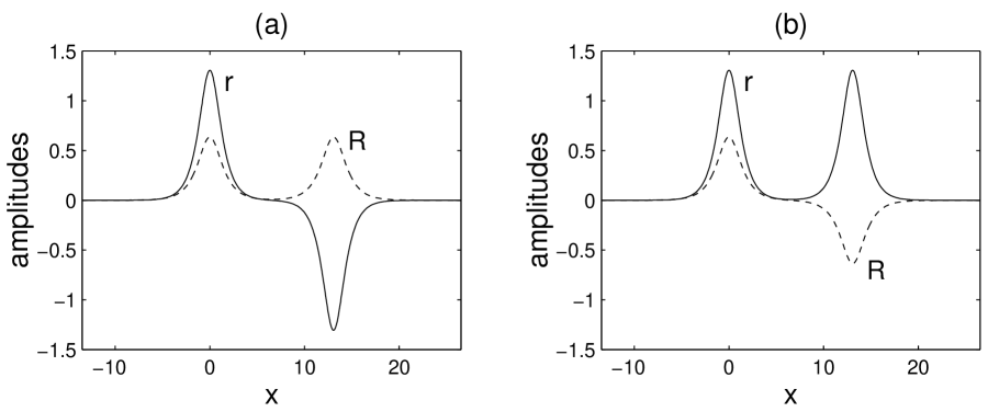
Figure 1: Numerically obtained stationary two-vector-soliton bound states at $\beta=2/3$ and $\Omega=0.85$: (a) type-I state; (b) type-II state. Analytical approximations by Eqs. (2.8), (2.9), and (2.10) are indistinguishable from the numerical curves and thus not shown.

Analytical construction of multi-soliton bound states in a general nonlinear wave system was made in [18] using a tail-matching method, and the spacing formula (2.10) for the coupled NLS equations was derived only as a special case (see [24] for an application of this method for the construction of other types of multi-pulse bound states). Below, we use a simplified version of [18]’s method to construct multi-vector-soliton bound states in the coupled NLS equations [i.e., (2.4) and (2.5)], and reproduce the spacing formula (2.10). There are two reasons for our doing this: (i) to highlight the key ideas in the tail-matching method for the construction of multi-pulse bound states; (ii) to motivate a similar tail-matching idea for the linear-stability analysis of multi-pulse bound states (see Sec. 3).

Suppose we have a bound state of two vector solitons located at $x=0$ and $\Delta\>(\gg 1)$. As $\Delta\to\infty$, the leading-order asymptotics of this bound state is

$$r(x)\longrightarrow r_{0}(x)+s_{1}r_{0}(x-\Delta),\hskip 14.22636ptR(x)\longrightarrow R_{0}(x)+s_{2}R_{0}(x-\Delta),$$ (2.11)

where $s_{1}$ and $s_{2}$ are sign-constants and are either 1 or $-1$. Our task is to determine values of $s_{1},s_{2}$ and the spacing $\Delta$. For this purpose, we consider the bound state in two $x$-regions: $-\infty<x\ll\Delta$, and $0\ll x<\infty$. Since the treatments for these two regions are the same, we only look at the first region $-\infty<x\ll\Delta$. In this region, the bound state is a slightly perturbed fundamental vector soliton, i.e.,

$$r(x)=r_{0}(x)+\tilde{r}(x),\hskip 14.22636ptR(x)=R_{0}(x)+\tilde{R}(x),$$ (2.12)

where $\tilde{r},\tilde{R}\ll 1$. The actual forms and sizes of $\tilde{r}$ and $\tilde{R}$ are not important in this analysis, but their asymptotics in the region $x\sim\frac{1}{2}\Delta\gg 1$ is crucial. This asymptotics can be obtained by matching $[r(x),R(x)]$’s expressions (2.12) with their asymptotics (2.11). This is the key idea of the method. This matching gives the leading-order asymptotics of $(\tilde{r},\tilde{R})$ as

$$\left[\begin{array}[]{c}\tilde{r}(x)\\ \tilde{R}(x)\end{array}\right]\longrightarrow\left[\begin{array}[]{c}s_{1}r_{0}(x-\Delta)\\ s_{2}R_{0}(x-\Delta)\end{array}\right]\longrightarrow\left[\begin{array}[]{c}s_{1}c\>e^{x-\Delta}\\ s_{2}Ce^{\Omega(x-\Delta)}\end{array}\right],\hskip 17.07182ptx\sim\frac{1}{2}\Delta\gg 1.$$ (2.13)

As $x\to-\infty$, $(\tilde{r},\tilde{R})\to 0$.

When Eq. (2.12) is substituted into (2.4) and (2.5), and higher-order terms dropped, the linearized equations for perturbations $(\tilde{r},\tilde{R})$ are found to be

$$L\left[\begin{array}[]{c}\tilde{r}\\ \tilde{R}\end{array}\right]=0,$$ (2.14)

where the linearization operator $L$ is

$$L=\left[\begin{array}[]{cc}\partial_{xx}-1+3r_{0}^{2}(x)+\beta R_{0}^{2}(x)&2r_{0}(x)R_{0}(x)\\ 2r_{0}(x)R_{0}(x)&\partial_{xx}-\Omega^{2}+3R_{0}^{2}(x)+\beta r_{0}^{2}(x)\end{array}\right],$$ (2.15)

which is self-adjoint. Eq. (2.14) has one localized homogeneous solution $[r^{\prime}_{0}(x),R^{\prime}_{0}(x)]^{\mbox{\scriptsize T}}$ when $\beta\neq 0$ and 1. Here the prime is the derivative, and the superscript “T” is the transpose of a vector. Thus, in order for the solution $(\tilde{r},\tilde{R})$ of Eq. (2.14) to exist, a solvability condition

$$\int_{-\infty}^{x_{m}}[r^{\prime}_{0}(x),R^{\prime}_{0}(x)]L\left[\begin{array}[]{c}\tilde{r}\\ \tilde{R}\end{array}\right]dx=0$$ (2.16)

must be satisfied. Here $x_{m}\sim\frac{1}{2}\Delta$. This condition can be simplified through integration by parts as

$$\left[\tilde{r}^{\prime}(x)r^{\prime}_{0}(x)-\tilde{r}(x)r^{\prime\prime}_{0}(x)+\tilde{R}^{\prime}(x)R^{\prime}_{0}(x)-\tilde{R}(x)R^{\prime\prime}_{0}(x)\right]_{-\infty}^{x_{m}}=0.$$ (2.17)

Finally, substitution of the asymptotics (2.7) and (2.13) into the above condition gives

$$e^{-(1-\Omega)\Delta}=-\frac{s_{1}s_{2}C^{2}\Omega^{2}}{c^{2}}.$$ (2.18)

This equation readily shows that in order for the bound state to exist, we must have $s_{1}s_{2}=-1$. In that case, the spacing formula (2.18) becomes exactly the same as (2.10). Hence the above simplified tail-matching method reproduces the results from the more general analysis in [18].

The relative errors of the leading-order bound states (2.8), (2.9), and the spacing formula (2.10) have been discussed in [18], and these errors are $O(e^{-\Delta},e^{-\Omega\Delta})$. For the bound states, we have

$$r(x)=\left[r_{0}(x)\mp r_{0}(x-\Delta)\right]\left[1+O(e^{-\Delta},e^{-\Omega\Delta})\right],$$ (2.19)

$$R(x)=\left[R_{0}(x)\pm R_{0}(x-\Delta)\right]\left[1+O(e^{-\Delta},e^{-\Omega\Delta})\right].$$ (2.20)

These error estimates can also be obtained as follows. Let us consider the type-I bound state. Write

$$r(x)=r_{0}(x)-r_{0}(x-\Delta)+\hat{r}(x),$$ (2.21)

$$R(x)=R_{0}(x)+R_{0}(x-\Delta)+\hat{R}(x),$$ (2.22)

where $\hat{r},\hat{R}\ll 1$. Substituting these equations into (2.4) and (2.5), we find that in the region $-\infty<x\ll\Delta$,

$$L\left[\begin{array}[]{c}\hat{r}\\ \hat{R}\end{array}\right]=\left[\begin{array}[]{c}-\left[3r_{0}^{2}(x)+\beta R_{0}^{2}(x)\right]r_{0}(x-\Delta)+2\beta r_{0}(x)R_{0}(x)R_{0}(x-\Delta)\\ \left[3R_{0}^{2}(x)+\beta r_{0}^{2}(x)\right]R_{0}(x-\Delta)-2\beta r_{0}(x)R_{0}(x)r_{0}(x-\Delta),\end{array}\right].$$ (2.23)

Here terms which are higher-order than the ones kept in (2.23) have been dropped. A similar equation can be obtained in the region $0\ll x<\infty$. Inspection of these equations shows that for all values of $x$, $(\hat{r},\hat{R})$ is exponentially small compared to the leading-order terms in (2.8) and (2.9), and the relative errors are $O(e^{-\Delta},e^{-\Omega\Delta})$ as shown in (2.19) and (2.20).

The spacing formula (2.10) together with the results in [9] reveals that, in order for $\Delta\gg 1$, we must have $0<\beta<1$. In addition, we must have either $C/c\ll 1$, $\Omega<1$, or $C/c\gg 1$, $\Omega>1$. In the former limit, $R_{0}(x)\ll r_{0}(x)$, and $\Omega\approx\Omega_{c}$; while in the latter limit, $r_{0}(x)\ll R_{0}(x)$, and $\Omega\approx 1/\Omega_{c}$. In both limits, the bound states look like two wave-and-daughter-waves glued together. These two limits are actually equivalent through a scaling of variables (the so-called reciprocal relation in [9]). Thus in the rest of this article, we will just consider the former limit where $\Omega\approx\Omega_{c}$. Fundamental solitons in this limit have been perturbatively determined in [9]. Utilizing those results, we readily find that the asymptotic formula for the spacing $\Delta$ is

$$\Delta\longrightarrow\frac{1}{1-\Omega_{c}}\left\{-\ln(\Omega-\Omega_{c})+K+o(1)\right\},\hskip 11.38092pt\Omega\to\Omega_{c},$$ (2.24)

where the constant $K$ is

$$K=(3-2\Omega_{c})\ln 2-2\ln\Omega_{c}+\ln\gamma,$$

and

$$\gamma=\frac{(1-\Omega_{c}^{3})\int^{\infty}_{-\infty}\mbox{sech}^{4\Omega_{c}}xdx}{2\Omega_{c}\int^{\infty}_{-\infty}\mbox{sech}^{2\Omega_{c}}xdx}.$$ (2.25)

3 Linear-stability analysis of two-vector-soliton
bound states

To study the linear stability of the above two-vector-soliton bound states, we perturb these states as

$$A=e^{it}\left\{r(x)+\psi_{1}(x)e^{i\lambda t}+\psi_{2}^{*}(x)e^{-i\lambda^{*}t}\right\},$$ (3.1)

$$B=e^{i\Omega^{2}t}\left\{R(x)+\psi_{3}(x)e^{i\lambda t}+\psi_{4}^{*}(x)e^{-i\lambda^{*}t}\right\},$$ (3.2)

where $[r(x),R(x)]$ is a two-vector-soliton bound state, $\psi_{k}\;(1\leq k\leq 4)$ are infinitesimal disturbances, $\lambda$ is the eigenvalue, and $\psi^{*}$ is the complex conjugate of $\psi$. Substituting these equations into (2.1) and (2.2) and dropping higher-order terms, we get the following eigenvalue relation

$${\cal L}\Psi=\lambda\Psi,$$ (3.3)

where the linearization operator ${\cal L}$ is

$${\cal L}=\left(\begin{array}[]{cccc}\partial_{xx}-1+2r^{2}+\beta R^{2}&r^{2}&\beta rR&\beta rR\\ -r^{2}&-\partial_{xx}+1-2r^{2}-\beta R^{2}&-\beta rR&-\beta rR\\ \beta rR&\beta rR&\partial_{xx}-\Omega^{2}+2R^{2}+\beta r^{2}&R^{2}\\ -\beta rR&-\beta rR&-R^{2}&-\partial_{xx}+\Omega^{2}-2R^{2}-\beta r^{2}\end{array}\right),$$ (3.4)

and $\Psi=(\psi_{1},\psi_{2},\psi_{3},\psi_{4})^{\mbox{\scriptsize T}}$. The spectrum of ${\cal L}$ contains all information on the linear stability of the two-vector-soliton bound state. If ${\cal L}$ has eigenvalues with Im($\lambda)<0$, then the bound state is linearly unstable; otherwise, it is linearly stable. Obviously, the continuous spectrum of ${\cal L}$ always lies on the real axis, thus we only need to look at the discrete eigenvalues of ${\cal L}$. Notice that ${\cal L}^{2}$ is self-adjoint, thus ${\cal L}$’s eigenvalues are either purely real, or purely imaginary. In addition, if $\lambda$ is an eigenvalue of ${\cal L}$, so are $-\lambda$. Hence ${\cal L}$’s eigenvalues always come in pairs on the real or imaginary axis.

It is insightful to view ${\cal L}$’s discrete eigenvalues for the bound states $(r,R)$ in the perspective of eigenvalue bifurcations from a similar operator ${\cal L}_{0}$ for fundamental vector solitons $(r_{0},R_{0})$. Here

$${\cal L}_{0}={\cal L}|_{(r=r_{0},R=R_{0})}.$$ (3.5)

The spectrum structure of ${\cal L}_{0}$ has been determined completely in [12, 25]. This operator has 6 or 8 discrete eigenvalues (multiplicity counted), depending on whether an internal mode exists or not. The zero eigenvalue always has multiplicity 6 — three from position and phase invariances (Goldstein modes), and the other three from velocity and frequency (or equivalently, amplitude) variations. When an internal mode exists, a pair of real eigenvalues of opposite sign are present as well. If two vector solitons form a widely-separated stationary bound state $(\Delta\gg 1)$, both solitons must be either wave-and-daughter-waves (with $\Omega\approx\Omega_{c}$ and $0<\beta<1$), or having nearly equal amplitudes in the two components (with $\Omega\approx 1$ and $\beta>0$) [9, 39] (only the former type of bound states is studied in this paper). It has been shown in [25] that wave-and-daughter-waves do not admit internal modes. For instance, single vector solitons in Fig. 1’s bound states do not have internal modes [25]. Thus ${\cal L}_{0}$ has only a single discrete eigenvalue zero of multiplicity 6. In a bound state of two wave-and-daughter-waves, ${\cal L}$ will then have 12 discrete eigenvalues (multiplicities counted) — double that for a single wave-and-daughter-wave. Here, no new discrete eigenvalues of ${\cal L}$ can be generated from edge bifurcations of ${\cal L}_{0}$ because the edge points of ${\cal L}_{0}$’s continuous spectrum are not in the continuous spectrum. Now the zero eigenvalue of ${\cal L}$ still has multiplicity 6. Another six eigenvalues of ${\cal L}$ must bifurcate from zero due to tail interactions between solitons. Tracking of these six bifurcated eigenvalues will then provide a complete characterization of linear stability for these two-soliton bound states.

In this section, we propose a new and general tail-matching method to derive explicit analytical formulas for the six eigenvalues of ${\cal L}$ that bifurcate from zero, under the condition that the individual vector solitons in the bound state are widely separated. The idea of this method is to perturbatively determine the bifurcated eigenstate around each vector soliton. By matching their tail asymptotics in the center region of the eigenstate, their asymptotics in that region can then be explicitly obtained. Finally by utilizing the solvability conditions for the eigenstate, analytical formulas for the bifurcated eigenvalues will be derived. These formulas turn out to be exactly the same as those obtained by the KSGO method [21], but the present method is much simpler.

The bifurcated eigenvalues are of two types. One type consists of a pair of eigenvalues which bifurcate from the position-related zero eigenvalue. At infinite soliton separation, these eigenstates are equal to the sum of two position-induced Goldstein modes separated infinitely apart. The other type consists of two pairs of eigenvalues which bifurcate from the phase-related zero eigenvalue. At infinite soliton separation, these eigenstates are equal to the sum of two phase-induced Goldstein modes separated infinitely apart. These two types of eigenvalues have their counterparts in the linear stability analysis by the KSGO method [21].

Below, we consider eigenvalue bifurcations in type-I and II bound states. It turns out that eigenvalues of type-II bound states are simply equal to those of type-I states multiplied by $i$ (see also [21]). Thus calculations for only type-I states will be presented. These states are anti-symmetric in $r$, and symmetric in $R$, around the center of the bound states [see Fig. 1(a)]. When $\Delta\to\infty$,

$$r(x)\longrightarrow r_{0}(x)-r_{0}(x-\Delta),\hskip 14.22636ptR(x)\longrightarrow R_{0}(x)+R_{0}(x-\Delta).$$ (3.6)

Bifurcations of position- and phase-related eigenvalues are studied separately next.

3.1 Bifurcation of position-related eigenvalues

When $\Delta\to\infty$, the eigenstate bifurcated from the position-related zero eigenvalue is a sum of two position-induced Goldstein modes of fundamental vector solitons:

$$\Psi(x)\longrightarrow\Psi_{0}(x)+\hat{\Psi}_{0}(x),\hskip 14.22636pt\Delta\to\infty,$$ (3.7)

where

$$\Psi_{0}(x)=\left[\begin{array}[]{c}r^{\prime}_{0}(x)\\ r^{\prime}_{0}(x)\\ R^{\prime}_{0}(x)\\ R^{\prime}_{0}(x)\end{array}\right],\hskip 14.22636pt\hat{\Psi}_{0}(x)=\left[\begin{array}[]{c}r^{\prime}_{0}(x-\Delta)\\ r^{\prime}_{0}(x-\Delta)\\ -R^{\prime}_{0}(x-\Delta)\\ -R^{\prime}_{0}(x-\Delta)\end{array}\right].$$ (3.8)

The first two components of $\Psi$ are anti-symmetric around $x=\frac{1}{2}\Delta$, and the last two components are symmetric around $x=\frac{1}{2}\Delta$. Note that in the same limit, the eigenstate $\Psi_{0}(x)-\hat{\Psi}_{0}(x)$ is simply $[r^{\prime}(x),\;r^{\prime}(x),\;R^{\prime}(x),\;R^{\prime}(x)]^{\mbox{\scriptsize T}}$, which is the un-bifurcated Goldstein eigenmode with eigenvalue zero and is thus not considered.

In the limit $\Delta\gg 1$, we consider the bifurcated eigenstate in the region $-\infty<x\ll\Delta$, and expand it as a perturbation series in powers of the small eigenvalue $\lambda$:

$$\Psi(x)=\Psi_{0}(x)+\lambda\Psi_{1}(x)+\lambda^{2}\Psi_{2}(x)+o(\lambda^{2}),\hskip 22.76228pt-\infty<x\ll\Delta.$$ (3.9)

In this region, we also expand

$${\cal L}={\cal L}_{0}+\lambda^{2}{\cal L}_{2}+o(\lambda^{2}).$$ (3.10)

It is noted that when $\Delta\gg 1$, single solitons in the bound state considered are wave-and-daughter-waves whose two components have different orders (one component asymptotically much smaller than the other). This fact certainly has implications in the stability analysis. In particular, different components of $\Psi$ and ${\cal L}$ in the region $-\infty<x\ll\Delta$ may have slightly different orders of magnitude. Thus, a perturbation expansion with a more-detailed ordering of different components than that in (3.9) and (3.10) might be needed. But as we will see next, (3.9) and (3.10) still work.

Now we substitute the perturbation expansions (3.9) and (3.10) into the eigenvalue equation (3.3). At $O(1)$, we get ${\cal L}_{0}\Psi_{0}(x)=0$ which is satisfied automatically. At $O(\lambda)$, we get

$${\cal L}_{0}\Psi_{1}=\Psi_{0},$$ (3.11)

whose solution is

$$\Psi_{1}(x)=[\frac{1}{2}xr_{0}(x),\;\;-\frac{1}{2}xr_{0}(x),\;\;\frac{1}{2}xR_{0}(x),\;\;-\frac{1}{2}xR_{0}(x)]^{\mbox{\scriptsize T}}.$$ (3.12)

Note that this function is an inhomogeneous solution of Eq. (3.11). In general, $\Psi_{1}$ should also include the homogeneous solutions which are a linear combination of the three Goldstein modes: $\Psi_{0}(x)$ in (3.8), and [$\Phi_{0}^{(1)}(x)$, $\Phi_{0}^{(2)}(x)$] in (3.26). But the $\Psi_{0}(x)$ term in $\Psi_{1}$ can be combined with the $O(1)$ term in the expansion (3.9), and the other two Goldstein modes [$\Phi_{0}^{(1)}(x)$, $\Phi_{0}^{(2)}(x)$] are phase-related and do not arise here. Thus the solution of Eq. (3.11) can be taken as (3.12) without loss of generality.

At $O(\lambda^{2})$, we get

$${\cal L}_{0}\Psi_{2}=\Psi_{1}-{\cal L}_{2}\Psi_{0}.$$ (3.13)

It is more convenient to express ${\cal L}_{2}\Psi_{0}$ in a different form. Recall that the un-bifurcated position-related Goldstein mode $\Psi_{g}(x)$ of ${\cal L}$ has the leading-order asymptotics $\Psi_{0}(x)-\hat{\Psi}_{0}(x)$ for $\Delta\gg 1$. When this asymptotics and ${\cal L}$’s expansion (3.10) are substituted into the Goldstein-mode relation ${\cal L}\Psi_{g}(x)=0$, we find that asymptotically,

$$\lambda^{2}{\cal L}_{2}\Psi_{0}={\cal L}_{0}\hat{\Psi}_{0}.$$ (3.14)

Thus Eq. (3.13) can be rewritten as

$${\cal L}_{0}\left[\Psi_{2}+\lambda^{-2}\hat{\Psi}_{0}\right]=\Psi_{1}.$$ (3.15)

Note that ${\cal L}_{0}\hat{\Psi}_{0}$ is $O(\lambda^{2})$, thus the above equation is not dis-ordered.

The solvability condition of Eq. (3.15) will produce formulas for the eigenvalue $\lambda$. To do this, we need the asymptotics of function $\Psi_{2}$ in the region $x\sim\frac{1}{2}\Delta\gg 1$, which we derive using the tail-matching idea. We have known that $\Psi$’s leading-order asymptotics at $\Delta\gg 1$ is given by (3.7) for all values of $x$. Combining this asymptotics with the perturbation expansion (3.9) and solutions (3.8) and (3.12), we see that

$$\Psi_{2}(x)\to\frac{1}{\lambda^{2}}\hat{\Psi}_{0}(x),\hskip 14.22636ptx\sim\frac{1}{2}\Delta\gg 1.$$ (3.16)

Of course, $\Psi_{2}(x)\to 0$ when $x\to-\infty$.

The homogeneous equation of (3.15) has three linearly independent solutions which are the Goldstein modes $\Psi_{0}(x)$ in (3.8) and [$\Phi_{0}^{(1)}(x),\Phi_{0}^{(2)}(x)$] in (3.26). Thus Eq. (3.15) has three solvability conditions. These conditions can be readily derived by noting that diag$(1,-1,1,-1){\cal L}_{0}$ is self-adjoint. It turns out that two of the solvability conditions induced by the Goldstein modes [$\Phi_{0}^{(1)},\Phi_{0}^{(2)}$] are satisfied automatically. The remaining solvability condition reads,

$$\int_{-\infty}^{x_{m}}\langle\Psi_{0}|\mbox{diag}(1,-1,1,-1)|{\cal L}_{0}(\Psi_{2}+\lambda^{-2}\hat{\Psi}_{0})\rangle dx$$

$$=\int_{-\infty}^{x_{m}}\langle\Psi_{0}|\mbox{diag}(1,-1,1,-1)|\Psi_{1}\rangle dx,$$ (3.17)

where $x_{m}\sim\frac{1}{2}\Delta$, $\langle\cdot|$ and $|\cdot\rangle$ are the Dirac ket and bra notations [26]. Integrating by parts to its left-hand-side and simplifying its right-hand-side, we get

$$\left[\langle\Psi_{0}|(\Psi_{2x}+\lambda^{-2}\hat{\Psi}_{0x})\rangle-\langle\Psi_{0x}|(\Psi_{2}+\lambda^{-2}\hat{\Psi}_{0})\rangle\right]_{-\infty}^{x_{m}}=-\frac{1}{2}\int_{-\infty}^{x_{m}}(r_{0}^{2}+R_{0}^{2})dx.$$ (3.18)

The left-hand-side of (3.18) can be calculated using the asymptotics (2.7), (3.16) and equation (3.8), while the integral on the right-hand-side of (3.18) is asymptotically equal to a similar integral but with the upper limit $x_{m}$ replaced by $\infty$. After these calculations, the eigenvalue $\lambda$ is finally found to be

$$\lambda^{2}=\frac{16(1-\Omega)c^{2}e^{-\Delta}}{M+N},$$ (3.19)

where $M$ and $N$ are the masses of the $r$ and $R$ components in a fundamental vector soliton:

$$M\equiv\int_{-\infty}^{\infty}r_{0}^{2}dx,\hskip 14.22636ptN\equiv\int_{-\infty}^{\infty}R_{0}^{2}dx.$$ (3.20)

We immediately see that formula (3.19) is identical to the one derived in [21] using the KSGO method. Thus, the present tail-matching method has the same accuracy as the KSGO method, but is only simpler. Recall that we only consider the $\Omega\approx\Omega_{c}(<1)$ limit. In this limit, the type-I state flips sign in its larger component, and does not flip sign in its smaller component [see Fig. 1(a)]. According to formula (3.19), this position-related eigenvalue $\lambda$ is real, thus it does not create instability. A comparison between the analytical formula (3.19) and numerical values at $\beta=\frac{2}{3}$ has been made in [21], and excellent agreement has been obtained.

Formula (3.19) shows that $\lambda=O(e^{-\frac{1}{2}\Delta})$. When $\Omega\to\Omega_{c}$ and $0<\beta<1$, $\Delta\to\infty$ (see Sec. 2). In this limit, the asymptotic formula for $\lambda$ can be obtained more explicitly from (2.24) and (3.19) as

$$\lambda^{2}\longrightarrow\alpha\>(\Omega-\Omega_{c})^{\frac{1}{1-\Omega_{c}}},\hskip 14.22636pt\Omega\to\Omega_{c},$$ (3.21)

where the constant $\alpha$ is

$$\alpha=32(1-\Omega_{c})\left(\frac{\Omega_{c}^{2}4^{\Omega_{c}}}{8\gamma}\right)^{\frac{1}{1-\Omega_{c}}}.$$ (3.22)

Here $\Omega_{c}$ and $\gamma$ are defined in Eqs. (2.6) and (2.25).

3.2 Bifurcation of phase-related eigenvalues

Calculations for the bifurcation of phase-related eigenvalues are quite similar to that done above. In this case, the eigenmode has the following asymptotics:

$$\Psi(x)\longrightarrow\Phi_{0}(x)+\hat{\Phi}_{0}(x),\hskip 14.22636pt\Delta\to\infty,$$ (3.23)

where

$$\Phi_{0}(x)=\Phi_{0}^{(1)}(x)+\delta\Phi_{0}^{(2)}(x),$$ (3.24)

$$\hat{\Phi}_{0}(x)=\Phi_{0}^{(1)}(x-\Delta)-\delta\Phi_{0}^{(2)}(x-\Delta),$$ (3.25)

$$\Phi_{0}^{(1)}(x)=\left[\begin{array}[]{c}r_{0}(x)\\ -r_{0}(x)\\ 0\\ 0\end{array}\right],\hskip 14.22636pt\Phi_{0}^{(2)}(x)=\left[\begin{array}[]{c}0\\ 0\\ R_{0}(x)\\ -R_{0}(x)\end{array}\right],$$ (3.26)

and $\delta$ is some constant (to be determined). The first two components of this mode are symmetric around $x=\frac{1}{2}\Delta$, and the last two components are anti-symmetric around $x=\frac{1}{2}\Delta$. Note that the eigenstate with asymptotics $\Phi_{0}(x)-\hat{\Phi}_{0}(x)$ is simply $[r(x),\;-r(x),\;\delta R(x),\;-\delta R(x)]^{\mbox{\scriptsize T}}$, which is the un-bifurcated Goldstein eigenmode with eigenvalue zero and is not a concern.

Next, we construct a perturbation-series solution for $\Psi(x)$ in the region $-\infty<x\ll\Delta$. The perturbation series is similar to (3.9):

$$\Psi(x)=\Phi_{0}(x)+\lambda\Phi_{1}(x)+\lambda^{2}\Phi_{2}(x)+o(\lambda^{2}),\hskip 22.76228pt-\infty<x\ll\Delta,$$ (3.27)

where $\Phi_{0}(x)$ is given by (3.24). Substituting this expansion and (3.10) into the eigenvalue relation (3.3), the $O(1)$ equation is satisfied automatically. At $O(\lambda)$, we get

$${\cal L}_{0}\Phi_{1}=\Phi_{0},$$ (3.28)

whose solution is

$$\Phi_{1}(x)=\frac{1}{2}\frac{\partial}{\partial\omega}\left[\begin{array}[]{c}r_{0}(x;\omega,\Omega)\\ r_{0}(x;\omega,\Omega)\\ R_{0}(x;\omega,\Omega)\\ R_{0}(x;\omega,\Omega)\end{array}\right]_{\omega=1}+\frac{\delta}{2\Omega}\frac{\partial}{\partial\Omega}\left[\begin{array}[]{c}r_{0}(x;\omega,\Omega)\\ r_{0}(x;\omega,\Omega)\\ R_{0}(x;\omega,\Omega)\\ R_{0}(x;\omega,\Omega)\end{array}\right]_{\omega=1}.$$ (3.29)

Here $(r_{0},R_{0})$ is the fundamental vector soliton obtained from ODEs (2.4) and (2.5) without rescaling of $\omega=1$. Again, the homogeneous solution of Eq. (3.28), which is a linear combination of Goldstein modes $\Psi_{0}(x)$ in (3.8) and [$\Phi_{0}^{(1)}(x),\Phi_{0}^{(2)}(x)$] in (3.26), is not included because the latter modes can be absorbed into the $O(1)$ term in the perturbation expansion (3.27), and the former mode does not arise.

At $O(\lambda^{2})$, we get

$${\cal L}_{0}\Phi_{2}=\Phi_{1}-{\cal L}_{2}\Phi_{0}.$$ (3.30)

Again, utilizing the un-bifurcated phase-related Goldstein modes of ${\cal L}$ with asymptotics $\Phi_{0}(x)-\hat{\Phi}_{0}(x)$ — similar to what we have done in Sec. 3.1, we can rewrite ${\cal L}_{2}\Phi_{0}$ so that Eq. (3.30) becomes

$${\cal L}_{0}\left[\Phi_{2}+\lambda^{-2}\hat{\Phi}_{0}\right]=\Phi_{1}.$$ (3.31)

This equation has three solvability conditions induced by the three Goldstein modes in the homogeneous solution. The condition induced by the mode $\Psi_{0}(x)$ in (3.8) is satisfied automatically. The other two conditions are

$$\int_{-\infty}^{x_{m}}\langle\Phi_{0}^{(k)}|\mbox{diag}(1,-1,1,-1)|{\cal L}_{0}(\Phi_{2}+\lambda^{-2}\hat{\Phi}_{0})\rangle dx$$

$$=\int_{-\infty}^{x_{m}}\langle\Phi_{0}^{(k)}|\mbox{diag}(1,-1,1,-1)|\Phi_{1}\rangle dx,$$ (3.32)

where $x_{m}\sim\frac{1}{2}\Delta$, and $k=1,2$. Integration by parts simplifies these conditions as

$$\left[\langle\Phi_{0}^{(1)}|(\Phi_{2x}+\lambda^{-2}\hat{\Phi}_{0x})\rangle-\langle\Phi_{0x}^{(1)}|(\Phi_{2}+\lambda^{-2}\hat{\Phi}_{0})\rangle\right]_{-\infty}^{x_{m}}=\frac{1}{2}M_{\omega}+\frac{\delta}{2\Omega}M_{\Omega},$$ (3.33)

and

$$\left[\langle\Phi_{0}^{(2)}|(\Phi_{2x}+\lambda^{-2}\hat{\Phi}_{0x})\rangle-\langle\Phi_{0x}^{(2)}|(\Phi_{2}+\lambda^{-2}\hat{\Phi}_{0})\rangle\right]_{-\infty}^{x_{m}}=\frac{1}{2}N_{\omega}+\frac{\delta}{2\Omega}N_{\Omega}.$$ (3.34)

To calculate the left-hand-sides of the above two equations, we need the asymptotics of function $\Phi_{2}(x)$ in the region $x\sim\frac{1}{2}\Delta$. This asymptotics can be obtained by comparing $\Psi(x)$’s asymptotics (3.23) with its perturbation expansion (3.27). This comparison shows that $\Phi_{2}(x)$ must have the asymptotics

$$\Phi_{2}(x)\to\frac{1}{\lambda^{2}}\hat{\Phi}_{0}(x),\hskip 14.22636ptx\sim\frac{1}{2}\Delta\gg 1.$$ (3.35)

When this asymptotics as well as (2.7) is substituted into Eqs. (3.33) and (3.34) and parameter $\delta$ eliminated, the eigenvalue $\lambda$ is then given by the quartic equation

$$\lambda^{4}-\frac{16c^{2}(N_{\Omega}-M_{\omega})e^{-\Delta}}{M_{\omega}N_{\Omega}-M_{\Omega}N_{\omega}}\lambda^{2}-\frac{16^{2}c^{4}e^{-2\Delta}}{M_{\omega}N_{\Omega}-M_{\Omega}N_{\omega}}=0.$$ (3.36)

Again, this formula for phase-related eigenvalues is identical to that obtained in [21] by the KSGO method. As pointed in [21], this formula shows that a two-vector-soliton bound state always has one phase-related unstable eigenvalue which bifurcates from zero, thus is always linearly unstable. Comparison between this formula and numerical values has also been made in [21], and excellent agreement has been observed.

Formula (3.36) shows that phase-related eigenvalues $\lambda=O(e^{-\frac{1}{2}\Delta})$, the same as position-related eigenvalues [see Eq. (3.19)]. The asymptotics of these eigenvalues in the limit $\Omega\to\Omega_{c}$ can also be obtained from (2.24) and (3.36), but is not pursued here.

Next, we briefly discuss the linear stability of type-II vector-soliton bound states [see Fig. 1(b)]. In the limit of large separation, these solitons have the asymptotics

$$r(x)\longrightarrow r_{0}(x)+r_{0}(x-\Delta),\hskip 14.22636ptR(x)\longrightarrow R_{0}(x)-R_{0}(x-\Delta).$$ (3.37)

Repeating the above analytical calculations, we find that the eigenvalues for type-II states are equal to those of type-I states multiplied by $i$. Thus type-II states are always linearly unstable as well. But different from type-I states, the instability of type-II states in the limit $\Omega\approx\Omega_{c}(<1)$ is caused by two unstable eigenvalues: one related to position-mode bifurcations [see (3.19)], and the other one related to phase-mode bifurcations [see (3.36)]. This result agrees with that by the KSGO method as well as the numerical result [21].

4 Discussion

In this paper, we have analytically studied the linear stability of two-vector-soliton bound states in the coupled NLS equations by a new tail-matching method. Under the condition that the two vector solitons are wave-and-daughter-waves and are widely separated, we have calculated small eigenvalues of these bound states that bifurcate from the zero eigenvalue of single vector solitons. These small eigenvalues calculated are all the discrete non-zero eigenvalues of the bound states. We have shown that these bound states are always linearly unstable due to the existence of one unstable phase-induced eigenvalue. The analytical formulas for eigenvalues derived from this tail-matching method turn out to be exactly the same as those from the KSGO method [21], but the present method is much simpler. Even though our calculations were performed for two-vector-soliton bound states, these calculations can apparently be generalized to $n$-vector-soliton bound states.

This tail-matching method for the linear stability analysis of multi-soliton bound states is apparently quite general, and it can be applied to a wide range of other wave systems where similar multi-pulse bound states have been reported [18, 27, 28]. In addition, this method should be applicable to the stability analysis of other types of multi-pulses from nonlocal bifurcations in coupled-NLS-type equations [24]. Preliminary linear stability results through numerical studies shows that such multi-pulses are also linearly unstable [24], consistent with the results of the present article. This tail-matching method can also be used to calculate eigenvalue bifurcations of multi-pulses from internal modes (non-zero eigenvalues) of single pulses — a bifurcation which incidentally does not arise in the present problem because internal modes do not exist in single wave-and-daughter-waves [25].

Under what conditions can this tail-matching method give useful results? The main condition is that the individual pulses in the multi-pulse bound state are widely separated. This condition will dictate in what parameter regions such multi-pulses can exist, and thus tail-matching can proceed. For instance, for the coupled NLS equations (2.1) and (2.2), the spacing formulas (2.10) and (2.24) dictate that widely-separated multi-vector-soliton bound states ($\Delta\gg 1$) exist when $\Omega$ is near the local bifurcation boundary $\Omega=\Omega_{c}$. This is precisely the parameter region where our tail-matching linear stability analysis is performed.

The two-vector-soliton bound states studied in this paper reside outside the continuous spectrum of the corresponding linear-wave system. It is known that multi-pulse embedded solitons residing inside the continuous spectrum exist in various wave systems as well [29, 30, 31, 32, 33]. An interesting open issue is whether the tail-matching method can also be applied to the linear stability analysis of such multi-pulse embedded solitons. In the third-order NLS equation, it has been shown numerically that such embedded solitons are all linearly stable, but nonlinearly semi-stable [33].

Lastly, we relate this tail-matching method to other existing techniques for the linear stability analysis of multi-pulse bound states. Currently, the following techniques exist: the KSGO method [21], the dynamical-system method [34, 35], and the effective-interaction-potential method [36, 37, 38]. The present method is asymptotically accurate. It gives the same results as the KSGO method, but is much simpler. The dynamical-system method can count the number of unstable eigenvalues, or express the eigenvalues as the zeros of the Evans function. But it generally does not produce explicit formulas for eigenvalues. The effective-potential method can only capture position-related eigenvalue bifurcations, not phase-related eigenvalue bifurcations. (For the coupled NLS equations, phase-related eigenvalues are more important). In view of this comparison, we feel that the tail-matching method for the linear stability of multi-soliton bound states is very promising.

References

- [1] C.R. Menyuk, “Nonlinear pulse propagation in birefringent optical fibers.” IEEE J. Quantum Electron, QE-23, 174 (1987).
- [2] G.P. Agrawal, Nonlinear Fiber Optics. Academic Press, San Diego, 1989.
- [3] A. Hasegawa and Y. Kodama, Solitons in optical communications. Clarendon, Oxford, 1995.
- [4] C. Anastassiou, M. Segev, K. Steiglitz, J.A. Giordmaine, M. Mitchell, M. Shih, S. Lan and J. Martin, “Energy exchange interactions between colliding vector solitons.” Phys. Rev. Lett. 83, 2332 (1999).
- [5] E. A. Ostrovskaya, Yu. S. Kivshar, D. V. Skryabin, and W. J. Firth, “Stability of Multihump Optical Solitons.” Phys. Rev. Lett. 83, 296-299 (1999).
- [6] D.J. Benney, and A.C. Newell, “The propagation of nonlinear wave envelopes.” J. Math. Phys. 46, 133-139 (1967).
- [7] G.J. Roskes, “Some nonlinear multiphase interactions.” Stud. Appl. Math. 55, 231-238 (1976).
- [8] C.R. Menyuk, “Stability of solitons in birefringent optical fibers. II. Arbitrary amplitudes.” J. Opt. Soc. Am. B 5, 392 (1988).
- [9] J. Yang, “Classification of the solitary waves in coupled nonlinear Schroedinger equations.” Physica D, 108, 92–112 (1997).
- [10] Ueda, T. and Kath, W.L. “Dynamics of coupled solitons in nonlinear optical fibers.” Phys. Rev. A 42, 563 (1990).
- [11] D.J. Kaup, B.A. Malomed, and R.S. Tasgal, “Internal dynamics of a vector soliton in a nonlinear optical fiber.” Phys. Rev. E 48, 3049 (1993).
- [12] J. Yang, “Vector solitons and their internal oscillations in birefringent nonlinear optical fibers.” Stud. Appl. Math. 98, 61-97 (1997).
- [13] J. Yang and Y. Tan, “Fractal structure in the collision of vector solitons.” Phys. Rev. Lett. 85, 3624 (2000).
- [14] Y. Tan and J. Yang, “Complexity and regularity of vector-soliton collisions.” Phys. Rev. E. 64, 056616 (2001).
- [15] M. Haelterman, A.P. Sheppard and A.W. Snyder, “Bound vector solitary waves in isotropic nonlinear dispersive media.” Opt. Lett. 18, 1406 (1993).
- [16] V.E. Zakharov and A.B. Shabat, “Exact theory of two-dimensional self-focusing and one-dimensional self-modulation of waves in nonlinear media.” Sov. Phys. JETP 34, 62-69 (1972).
- [17] Z. Chen, M. Acks, E.A. Ostrovskaya and Y.S. Kivshar, “Observation of bound states of interacting vector solitons.” Opt. Lett. 25, 417 (2000).
- [18] J. Yang, “Multiple permanent-wave trains in nonlinear systems.” Stud. Appl. Math. 100, 127 (1998).
- [19] V.I. Karpman and V.V. Solov’ev, “A perturbation theory for soliton systems.” Physica D 3, 142 (1981).
- [20] K.A. Gorshkov and L.A. Ostrovsky, “Interactions of solitons in non-integrable systems: direct perturbation method and applications.” Physica D 3, 428 (1981).
- [21] J. Yang, “Interactions of vector solitons.” Phys. Rev. E 64, 026607 (2001).
- [22] S.V. Manakov, “On the theory of two-dimensional stationary self-focusing of electromagnetic waves.” Sov. Phys. JETP 38, 248-253 (1974).
- [23] J. Yang, and D.J. Benney, “Some properties of nonlinear wave systems.” Stud. Appl. Math. 96, 111-139 (1996).
- [24] A.R. Champneys and J. Yang, “A scalar nonlocal bifurcation of solitary waves for coupled nonlinear Schroedinger systems.” Nonlinearity 15, 2165 (2002).
- [25] D.E. Pelinovsky, and J. Yang, “Internal Oscillations and radiation damping of Vector Solitons.” Stud. Appl. Math. 105, 245 (2000).
- [26] P.A.M. Dirac, The Principles of Quantum Mechanics. Oxford Press, 1958.
- [27] A.R. Champneys and J.F. Toland, “Bifurcation of a plethora of multi-modal homoclinic orbits for autonomous Hamiltonian systems”. Nonlinearity 6, 665-721 (1993).
- [28] B. Buffoni, A.R. Champneys and J.F. Toland, “Bifurcation and coalescence of a plethora of homoclinic orbits for a Hamiltonian system.” Journal of Dynamics and Differential Equations 8, 221 (1996).
- [29] T.R. Akylas and T.J. Kung, “On nonlinear wave envelopes of permanent form near a caustic.” J. Fluid Mech. 214, 489 (1990).
- [30] M. Klauder, E.W. Laedke, K.H. Spatschek, and S.K. Turitsyn, “Pulse propagation in optical fibers near the zero dispersion point.” Phys. Rev. E 47, R3844 (1993).
- [31] D.C. Calvo and T.R. Akylas, “On the formation of bound states by interacting nonlocal solitary waves.” Physica D 101, 270 (1997).
- [32] K. Kolossovski, A.R. Champneys, A.V. Buryak, and R.A. Sammut, “Multipulse embedded solitons as bound states of quasi-solitons”. To appear in Physica D.
- [33] J. Yang and T.R. Akylas, “Continuous families of embedded solitons in the third-order nonlinear Schrödinger equation.” To appear in Stud. Appl. Math.
- [34] A. Yew, B. Sandstede and C.K.R.T. Jones. “Instability of multiple pulses in coupled nonlinear Schroedinger equations.” Phys. Rev. E 61, 5886 (2000).
- [35] B. Sandstede, “Stability of multiple-pulse solutions.” Trans. Am. Math. Soc. 350, 429 (1998).
- [36] B.A. Malomed, “Variational methods in nonlinear fiber optics and related fields.” Chapter 2, Progress in Optics 43, E.Wolf, editor (2002).
- [37] B.A. Malomed, “Bound solitons in the nonlinear Schrödinger–Ginzburg–Landau equation.” Phys. Rev. A 44, 6954 (1991).
- [38] A.V. Buryak and N.N. Akhmediev, “Stability criterion for stationary bound states of solitons with radiationless oscillating tails.” Phys. Rev. E 51, 3572 (1995).
- [39] J. Yang, “New families of solitary waves in the coupled nonlinear Schrödinger equations”, unpublished.
Department of Mathematics and Statistics
University of Vermont
Burlington, VT 05401, USA