Stability analysis of dynamical regimes in nonlinear systems with discrete symmetries

Abstract

We present a theorem that allows to simplify linear stability analysis of periodic and quasiperiodic nonlinear regimes in $N$-particle mechanical systems (both conservative and dissipative) with different kinds of discrete symmetry. This theorem suggests a decomposition of the linearized system arising in the standard stability analysis into a number of subsystems whose dimensions can be considerably less than that of the full system. As an example of such simplification, we discuss the stability of bushes of modes (invariant manifolds) for the Fermi-Pasta-Ulam chains and prove another theorem about the maximal dimension of the above mentioned subsystems.

I Introduction

Different dynamical regimes in a mechanical system with discrete-symmetry group $G_{0}$ can be classified by subgroups $G_{j}\subseteq G_{0}$ of this group DAN1 ; DAN2 ; PhysD . Actually, we can find an invariant manifold corresponding to each subgroup $G_{j}$ and decompose it into the basis vectors of the irreducible representations of the group $G_{0}$. As a result of this procedure, we obtain a bush of modes (see above cited papers) which can be considered as a certain physical object in geometrical, as well as dynamical sense. The mode structure of a given bush is fully determined by its symmetry group $G_{j}$ and is independent of the specific type of interparticle interactions in the system. In Hamiltonian systems, bushes of modes represent dynamical objects in which the energy of initial excitation turns out to be “trapped” (this is a phenomenon of energy localization in the modal space). The number of modes belonging to a given bush (the bush dimension) does not change in time, while amplitudes of the modes do change, and we can find dynamical equations determining their evolution.

Being an exact nonlinear excitation, in the considered mechanical system, each bush possesses its own domain of stability depending on the value of its mode amplitudes. Beyond the stability threshold a phenomenon similar to the parametric resonance occurs, the bush loses its stability and transforms into another bush of higher dimension. This process is accompanied by spontaneous lowering of the bush symmetry: $G_{j}\rightarrow\tilde{G_{j}}$, where $\tilde{G_{j}}\subset G_{j}$.

The concept of bushes of modes was introduced in DAN1 ; DAN2 , the detailed theory of these dynamical objects was developed in PhysD . Low-dimensional bushes in mechanical systems with various kinds of symmetry and structures were studied in DAN1 ; DAN2 ; PhysD ; IntJ ; ENOC ; Octa ; C60 ; FPU1 ; FPU2 . The problem of bush stability was discussed in PhysD ; Octa ; FPU1 ; FPU2 . Two last papers are devoted to the vibrational bushes in the Fermi-Pasta-Ulam (FPU) chains.

Note that dynamical objects equivalent to the bushes of modes were recently discussed for the monoatomic chains in the papers of different authors PR ; BR ; Shin ; AntiFPU . Let us emphasize that group-theoretical methods developed in our papers DAN1 ; DAN2 ; PhysD can be applied efficiently not only to the monoatomic chains (as was illustrated in FPU1 ; FPU2 ), but to all other physical systems with discrete symmetry groups (see, DAN1 ; DAN2 ; PhysD ; IntJ ; ENOC ; Octa ; C60 ).

In this paper, we present a theorem which can simplify essentially the stability analysis of the bushes of modes in complex systems with many degrees of freedom. The usefulness of this theorem is illustrated with the example of nonlinear chains with a large number of particles. Note that the simplification of the stability analysis in such systems actually originate from the well-known Wigner theorem about the block-diagonalization of the matrix commuting with all matrices of a representation of a given symmetry group.

In Sec. II, we start with the simplest examples for introducing basic concepts and ideas. In Sec. III, we present a general theorem about invariance of the dynamical equations linearized near a given bush with respect to the bush symmetry group. In Sec. IV, we prove a theorem which turns out to be very useful for splitting the above mentioned linearized dynamical equations for $N$-particle monoatomic chains. Some results on the bush stability in the FPU chains are discussed in Sec. V.

II Some simple examples

II.1 FPU-chains and their symmetry

We consider longitudinal vibrations of $N$-particle chains of identical masses ($m=1$) and identical springs connecting neighboring particles. Let $x_{i}(t)$ be the displacement of the $i$-th particle ($i=1,2,...,N$) from its equilibrium position at a given instance $t$. Dynamical equations of such mechanical system (FPU-chain) can be written as follows:

$$\ddot{x}_{i}=f(x_{i+1}-x_{i})-f(x_{i}-x_{i-1}).$$ (1)

The nonlinear force $f(x)$ depends on the deformation $x$ of the spring as $f(x)=x+x^{2}$ and $f(x)=x+x^{3}$ for the FPU-$\alpha$ and FPU-$\beta$ chains, respectively. We assume the periodic boundary conditions

$$x_{0}(t)\equiv x_{N}(t),\qquad x_{N+1}(t)\equiv x_{1}(t)$$ (2)

to be valid. Let us also introduce the “configuration vector” $\bm{X}(t)$ which is the $N$-dimensional vector describing all the displacements of the individual particles at the moment $t$:

$$\bm{X}(t)=\{x_{1}(t),x_{2}(t),\dots,x_{N}(t)\}.$$ (3)

In the equilibrium state, a given chain is invariant under the action of the operator $\hat{a}$ which shifts the chain by the lattice spacing $a$. This operator generates the translational group

$$T_{N}=\{\hat{e},\hat{a},\hat{a}^{2},\dotsc,\hat{a}^{N-1}\},\quad\hat{a}^{N}=\hat{e},$$ (4)

where $\hat{e}$ is the identity element and $N$ is the order of the cyclic group $T_{N}$. The operator $\hat{a}$ induces the cyclic permutation of all particles of the chain and, therefore, it acts on the “configuration vector” $\bm{X}(t)$ as follows:

$$\hat{a}\bm{X}(t)\equiv\hat{a}\{x_{1}(t),x_{2}(t),\dotsc,x_{N-1}(t),x_{N}(t)\}=\{x_{N}(t),x_{1}(t),x_{2}(t),\dotsc,x_{N-1}(t)\}.$$

The full symmetry group of the monoatomic chain contains also the inversion $\hat{\imath}$, with respect to the center of the chain, which acts on the vector $\bm{X}(t)$ in the following manner:

$$\hat{\imath}\bm{X}(t)\equiv\hat{\imath}\{x_{1}(t),x_{2}(t),\dotsc,x_{N-1}(t),x_{N}(t)\}=\{-x_{N}(t),-x_{N-1}(t),\dotsc,-x_{2}(t),-x_{1}(t)\}.$$

The complete set of all products $\hat{a}^{k}\hat{\imath}$ of the pure translations $\hat{a}^{k}$ ($k=0,1,2,\dotsc,N-1$) with the inversion $\hat{\imath}$ forms the so-called dihedral group $D_{N}$ which can be written as the direct sum of two cosets $T_{N}$ and $T_{N}\cdot\hat{\imath}$:

$$D_{N}=T_{N}\oplus T_{N}\cdot\hat{\imath}.$$ (5)

The dihedral group is a non-Abelian group induced by two generators ($\hat{a}$ and $\hat{\imath}$) with the following generating relations

$$\hat{a}^{N}=\hat{e},\quad\hat{\imath}^{2}=\hat{e},\quad\hat{\imath}\hat{a}=\hat{a}^{-1}\hat{\imath}.$$ (6)

We will consider different vibrational regimes in the FPU chains, which can be determined by the specific forms of the configuration vector. Each of these regimes depends on $m$ independent parameters ($m\leq N$) and this number is the dimension of the given regime.

The simplest case of one-dimensional vibrational regimes represents the so-called $\pi$-mode (zone boundary mode) :

$$\bm{X}(t)=\{A(t),-A(t)~{}|~{}A(t),-A(t)~{}|~{}A(t),-A(t)~{}|~{}\dots\},$$ (7)

where $A(t)$ is a certain function of $t$. In our terminology, this is the one-dimensional bush B$[\hat{a}^{2},\hat{\imath}]$ (see below about notation of bushes of modes).

The vector

$$\bm{X}(t)=\{0,A(t),B(t),0,-B(t),-A(t)~{}|~{}\dots\},$$ (8)

represents a two-dimensional vibrational regime that is determined by two time-dependent functions $A(t)$ and $B(t)$. This is the two-dimensional bush B$[\hat{a}^{6},\hat{a}\hat{\imath}]$ (see FPU2 ).

In general, for $m$-dimensional vibrational regime, we write $\bm{X}(t)=\bm{C}(t)$, where the $N$-dimensional vector $\bm{C}(t)$ depends on $m$ time-dependent functions only. Each specific dynamical regime $\bm{C}(t)$, being an invariant manifold, possesses its own symmetry group that is a subgroup of the parent symmetry group $G_{0}=D_{N}$ of the chain in equilibrium.

II.2 FPU-$\alpha$ chain with $N=4$ particles: existence of the bush B$[\hat{a}^{2},\hat{\imath}]$

Let us consider the above discussed equations for the simplest case $N=4$. Dynamical equations (1) read:

$$\begin{array}[]{l}\ddot{x}_{1}=f(x_{2}-x_{1})-f(x_{1}-x_{4}),\\ \ddot{x}_{2}=f(x_{3}-x_{2})-f(x_{2}-x_{1}),\\ \ddot{x}_{3}=f(x_{4}-x_{3})-f(x_{3}-x_{2}),\\ \ddot{x}_{4}=f(x_{1}-x_{4})-f(x_{4}-x_{3}).\end{array}$$ (9)

The symmetry group $G_{0}$ in the equilibrium state reads:

$$G_{0}=D_{4}=[\hat{a},\hat{\imath}]=\{\hat{e},\hat{a},\hat{a}^{2},\hat{a}^{3},\hat{\imath},\hat{a}\hat{\imath},\hat{a}^{2}\hat{\imath},\hat{a}^{3}\hat{\imath}\}.$$

Hereafter, we write generators of any symmetry group in square brackets, while all its elements (if it is necessary) are given in curly brackets.

The operators $\hat{a}$ and $\hat{\imath}$ act on the configuration vector $\bm{X}=\{x_{1},x_{2},x_{3},x_{4}\}$ as follows

$$\hat{a}\bm{X}=\{x_{4},x_{1},x_{2},x_{3}\},\qquad\hat{\imath}\bm{X}=\{-x_{4},-x_{3},-x_{2},-x_{1}\}.$$

Therefore, we can associate the following matrices $\mathrm{M}(\hat{a})$ and $\mathrm{M}(\hat{\imath})$ of the mechanical representation with these generators:

$$\hat{a}\Rightarrow\mathrm{M}(\hat{a})=\left(\begin{array}[]{rrrr}0&0&0&1\\ 1&0&0&0\\ 0&1&0&0\\ 0&0&1&0\\ \end{array}\right),\qquad\hat{\imath}\Rightarrow\mathrm{M}(\hat{\imath})=\left(\begin{array}[]{rrrr}0&0&0&-1\\ 0&0&-1&0\\ 0&-1&0&0\\ -1&0&0&0\\ \end{array}\right).$$ (10)

Their action on the configuration vector $\bm{X}$ is equivalent to that of the operators $\hat{a}$ and $\hat{\imath}$, respectively.

Let us now make the transformations of variables in the system (9) according to the action of the matrices (10), i.e.

$$\mathrm{M}(\hat{a}):x_{1}\rightarrow x_{4},\quad x_{2}\rightarrow x_{1},\quad x_{3}\rightarrow x_{2},\quad x_{4}\rightarrow x_{3},$$ (11)

$$\mathrm{M}(\hat{\imath}):x_{1}\rightarrow-x_{4},\quad x_{2}\rightarrow-x_{3},\quad x_{3}\rightarrow-x_{2},\quad x_{4}\rightarrow-x_{1}.$$ (12)

It is easy to check that both transformations (11) and (12) produce systems of equations which are equivalent to the system (9). Moreover, these transformations act on the individual equations $u_{j}$ ($j=1,2,3,4$) of the system (9) exactly as on the components $x_{j}$ ($j=1,2,3,4$) of the configuration vector $\bm{X}$. For example, for the operator $\hat{\imath}$ (or matrix $\mathrm{M}(\hat{\imath})$) we have

$$\hat{\imath}u_{1}=-u_{4},\quad\hat{\imath}u_{2}=-u_{3},\quad\hat{\imath}u_{3}=-u_{2},\quad\hat{\imath}u_{4}=-u_{1}.$$

It is obvious that a certain transposition of these equations multiplied by $\pm 1$ will indeed, produce a system fully identical to the original system (9). Thus, we are convinced that the symmetry group $G_{0}=D_{4}$ of our chain in equilibrium turns out to be the symmetry group (the group of invariance) of the dynamical equations of this mechanical system.

Let us now consider the vibrational regime (7), i.e. $\pi$-mode, and check that it represents an invariant manifold for the dynamical system (9). Substituting $x_{1}(t)=x_{3}(t)=A(t)$, $x_{2}(t)=x_{4}(t)=-A(t)$ into (9), we reduce these equations to one and the same equation of the form

$$\ddot{A}=f(-2A)-f(2A).$$ (13)

In the case of the FPU-$\alpha$ model this equation turns out to be the equation of harmonic oscillator (for the FPU-$\beta$ model it reduces to the Duffing equation). Indeed, for the FPU-$\alpha$ chain, we obtain from the Eq.(13):

$$\ddot{A}+4A=0.$$ (14)

Using, for simplicity, the initial condition $A(0)=C_{0}$, $\dot{A}(0)=0$, we get the following solution to Eq. (14):

$$A(t)=C_{0}\cos(2t).$$ (15)

Thus, the one-dimensional bush B$[\hat{a}^{2},\hat{\imath}]$ (or $\pi$-mode) (7) for the FPU-$\alpha$ chain, represents purely harmonic dynamical regime

$$\bm{X}(t)=C_{0}\{\cos(2t),-\cos(2t)~{}|~{}\cos(2t),-\cos(2t)\}.$$ (16)

On the other hand, the invariant manifold $\bm{X}(t)=\{A(t),-A(t),A(t),-A(t)\}$, corresponding to the bush B$[\hat{a}^{2},\hat{\imath}]$, can be obtained with the aid of the group-theoretical methods only, without consideration of the dynamical equations (9). Let us discuss this point in more detail.

At an arbitrary instant $t$, the displacement pattern $\{A(t),-A(t),A(t),-A(t)\}$ possesses its own symmetry group $G=D_{2}\subset G_{0}=D_{4}$. Indeed, this pattern is conserved under inversion ($\hat{\imath}$) and under shifting all particles by $2a$. The latter procedure can be considered as a result of the action on the chain by the operator $\hat{a}^{2}$. These two symmetry elements ($\hat{a}^{2}$ and $\hat{\imath}$) determine the dihedral group $D_{2}$ which is a subgroup of order two of the original group $G_{0}=D_{4}$ .

It is obvious, that the old element $\hat{a}$ of the group $G_{0}$, describing the chain in equilibrium, does not survive in the vibrational state described by the pattern (7). Note that this element ($\hat{a}$) transforms the regime (7) into its equivalent (but different!) form $\{-A(t),A(t),-A(t),A(t)\}$. In the present paper, we will not discuss different equivalent forms of bushes of modes (a detailed consideration of this problem can be found in FPU2 ). Thus, we encounter the reduction of symmetry $G_{0}=D_{4}\rightarrow G=D_{2}$ when we pass from the equilibrium state to the vibrational state (7) for the considered mechanical system.

The dynamical regime (7) represents the one-dimensional bush consisting of only one mode ($\pi$-mode). We will denote it as B$[G]$=B$[\hat{a}^{2},\hat{\imath}]:~{}\{A,-A,A,-A\}$. In square brackets, the group of the bush symmetry is indicated by listing its generators ($\hat{a}^{2}$ and $\hat{\imath}$, in our case), while the characteristic fragment of the bush displacement pattern is presented next to the colon. The bush symmetry group $G$ fully determines the form (displacement pattern) of the bush B$[G]$ (see, for example, PhysD ; FPU2 ). Indeed, in the case of the bush B$[\hat{a}^{2},\hat{\imath}]$, it is easy to show that this form, $\bm{X}=\{A(t),-A(t),A(t),-A(t)\}$, can be obtained as the general solution to the following linear algebraic equation representing the invariance of the configuration vector $\bm{X}$: $\hat{g}_{1}\bm{X}=\bm{X}$, $\hat{g}_{2}\bm{X}=\bm{X}$, where $\hat{g}_{1}=\hat{a}^{2}$ and $\hat{g}_{2}=\hat{\imath}$ are the generators of the group $G$. In our previous papers we often write these invariance conditions for the bush B$[G]$ in the form

$$\hat{G}\bm{X}=\bm{X}.$$ (17)

It is very essential, that the invariant vector $\bm{X}(t)$, which was found in such geometrical (group-theoretical) manner, turns out to be an invariant manifold for the considered dynamical system PhysD . Thus, we can obtain the symmetry-determined invariant manifolds (bushes of modes) without any information on interparticle interactions in the mechanical system.

II.3 FPU-$\alpha$ chain with $N=4$ particles: stability of the bush B$[\hat{a}^{2},\hat{\imath}]$

We now turn to the question of the stability of the bush B$[\hat{a}^{2},\hat{\imath}]$, representing a periodic vibrational regime $\bm{X}=\{A(t),-A(t),A(t),-A(t)\}$, with $A(t)=C_{0}\cos(2t)$. According to the conventional prescription, we must linearize the dynamical system (9) in the infinitesimal vicinity of the given bush and then study the obtained system. For this goal, let us write

$$\bm{X}(t)=\bm{C}(t)+\bm{\delta}(t),$$ (18)

where $\bm{C}=\{A(t),-A(t),A(t),-A(t)\}$ represents our bush, while $\bm{\delta}(t)=\{\delta_{1}(t),\delta_{2}(t),\delta_{3}(t),\delta_{4}(t)\}$ is an infinitesimal vector. Substituting (18) into Eqs. (9) and neglecting all terms nonlinear in $\delta_{j}(t)$, we obtain the following linearized equations for the FPU-$\alpha$ model:

$$\begin{array}[]{l}\ddot{\delta}_{1}=[\delta_{2}-2\delta_{1}+\delta_{4}]-4A(t)\cdot[\delta_{2}-\delta_{4}],\\ \ddot{\delta}_{2}=[\delta_{3}-2\delta_{2}+\delta_{1}]+4A(t)\cdot[\delta_{3}-\delta_{1}],\\ \ddot{\delta}_{3}=[\delta_{4}-2\delta_{3}+\delta_{2}]-4A(t)\cdot[\delta_{4}-\delta_{2}],\\ \ddot{\delta}_{4}=[\delta_{1}-2\delta_{4}+\delta_{3}]+4A(t)\cdot[\delta_{1}-\delta_{3}].\end{array}$$ (19)

The last system of equations can be written in the form

$$\ddot{\bm{\delta}}=\mathrm{J}(t)\cdot\bm{\delta},$$ (20)

where $\mathrm{J}(t)$ is the Jacobi matrix for the system (9) calculated by the substitution of the vector $\bm{X}=\{A(t),-A(t),A(t),-A(t)\}$. This matrix can be presented as follows:

$$\mathrm{J}(t)=\mathrm{L}+4A(t)\cdot\mathrm{M},$$ (21)

where

$$\mathrm{L}=\left(\begin{array}[]{rrrr}-2&1&0&1\\ 1&-2&1&0\\ 0&1&-2&1\\ 1&0&1&-2\end{array}\right),\qquad\mathrm{M}=\left(\begin{array}[]{rrrrrr}0&-1&0&1\\ -1&0&1&0\\ 0&1&0&-1\\ 1&0&-1&0\end{array}\right)$$ (22)

are two time-independent symmetric matrices.

It easy to check that matrices $\mathrm{L}$ and $\mathrm{M}$ commute with each other: $\mathrm{L}\cdot\mathrm{M}=\mathrm{M}\cdot\mathrm{L}$. Therefore, there exists a time-independent orthogonal matrix $\mathrm{S}$ that transforms the both matrices $\mathrm{L}$ and $\mathrm{M}$ to the diagonal form: $\mathrm{\tilde{S}}\cdot\mathrm{L}\cdot\mathrm{S}=\mathrm{L}_{dia}$, $\mathrm{\tilde{S}}\cdot\mathrm{M}\cdot\mathrm{S}=\mathrm{M}_{dia}$ (here $\mathrm{\tilde{S}}$ is the transposed matrix with respect to $\mathrm{S}$). In turn, it means that the Jacobi matrix $\mathrm{J}(t)$ can be diagonalized at any time $t$ by one and the same time-independent matrix $\mathrm{S}$. Therefore, our linearized system (20) for the considered bush B$[\hat{a}^{2},\hat{\imath}]$ can be decomposed into four independent differential equations.

Let us discuss how the above matrix $\mathrm{S}$ can be obtain with the aid of the theory of irreducible representations of the symmetry group $G$ (in our case $G=D_{2}$).

In Sec. IV, we will consider a general method for obtaining the matrix $\mathrm{S}$ which reduces the Jacobi matrix $\mathrm{J}(t)$ to a block-diagonal form. This method uses the basis vectors of irreducible representations of the group $G$, constructed in the mechanical space of the considered dynamical system. In our simplest case of the monoatomic chain with $N=4$ particles, this method leads to the following result

$$\mathrm{S}=\frac{1}{2}\left(\begin{array}[]{rrrr}1&1&1&1\\ 1&1&-1&-1\\ 1&-1&1&-1\\ 1&-1&-1&1\end{array}\right).$$ (23)

The rows of the matrix $\mathrm{S}$ from (23) are simply the characters of four one-dimensional irreducible representations (irreps) – $\Gamma_{1}$, $\Gamma_{2}$, $\Gamma_{3}$, $\Gamma_{4}$ – of the Abelian group $D_{2}$, because each of these irreps is contained once in the decomposition of the mechanical representation of the group $G=D_{2}$. Introducing new variables $\bm{y}=\{y_{1},y_{2},y_{3},y_{4}\}$ instead of the old variables $\bm{\delta}=\{\delta_{1}(t),\delta_{2}(t),\delta_{3}(t),\delta_{4}(t)\}$ by the equation $\bm{y}=\mathrm{S}\cdot\bm{\delta}$ with $\mathrm{S}$ from (23), we arrive at the full splitting of the linearized equations (19) for the FPU-$\alpha$ model:

$$\ddot{y}_{1}=0,$$ (24a)

$$\ddot{y}_{2}=-2[1+4A(t)]y_{2},$$ (24b)

$$\ddot{y}_{3}=-4y_{3},$$ (24c)

$$\ddot{y}_{4}=-2[1-4A(t)]y_{4},$$ (24d)

where $A(t)=C_{0}\cos(2t)$.

With the aid of Eqs. (24), we can find the stability threshold in $C_{0}$ for loss of stability of the one-dimensional bush B$[\hat{a}^{2},\hat{\imath}]$. Indeed, according to Eqs. (24), the variables $y_{j}(t)$ ($j=1,2,3,4$) are independent from each other, and we can consider them in turn. Eq. (24a) for $y_{1}(t)$ describes the uniform motion of the center of masses of our chain, since it follows from the equations $\bm{y}=\mathrm{S}\cdot\bm{\delta}$ that $y_{1}(t)\sim(\delta_{1}(t)+\delta_{2}(t)+\delta_{3}(t)+\delta_{4}(t))$. Therefore, considering vibrational regimes only, we may assume $y_{1}(t)\equiv 0$.

If only $y_{3}(t)$ appears in the solution to the system (24), i.e. if $y_{1}(t)=0$, $y_{2}(t)=0$, $y_{4}(t)=0$, then we have from the equation $\bm{\delta}=\tilde{\mathrm{S}}\cdot\bm{y}$ (note that $\mathrm{S}$ is the orthogonal matrix and, therefore, $\mathrm{S}^{-1}=\tilde{\mathrm{S}}$): $\bm{\delta}(t)=\{y_{3}(t),-y_{3}(t),y_{3}(t),-y_{3}(t)\}$, where $y_{3}(t)\sim\cos(2t)$. This solution leads only to deviations “along” the bush $\bm{X}(t)=C_{0}\{\cos(2t),-\cos(2t),\cos(2t),-\cos(2t)\}$ and does not signify instability.

Since $A(t)=C_{0}\cos(2t)$, Eq. (24b) reads $\ddot{y}_{2}+[2+8C_{0}\cos(2t)]y_{2}=0$ and can be transformed to the standard form of the Mathieu equation, as well as Eq. (24d). Therefore, the stability threshold of the considered bush B$[\hat{a}^{2},\hat{\imath}]$ for $N=4$ can be determined directly from the well-known diagram of the regions of stable and unstable motion of the Mathieu equation. In such a way we can find that critical value $C_{c}$ for the amplitude $C_{0}$ of the given bush for which it loses its stability is $C_{c}$ =$0.303$.

In conclusion, let us focus on the point that turns out to be very important for proving the general theorem in Sec. III. The system (19) was obtained by linearizing the original system (9), near the dynamical regime $\bm{C}(t)=\{A(t),-A(t),A(t),-A(t)\}$, and Eqs. (9) are invariant with respect to the parent group $G_{0}=[\hat{a},\hat{\imath}]$. Despite this fact, Eqs. (19) are invariant only with respect to its subgroup $G=\{\hat{e},\hat{a}^{2},\hat{\imath},\hat{a}^{2}\hat{\imath}\}\subset G_{0}=\{\hat{e},\hat{a},\hat{a}^{2},\hat{a}^{3},\hat{\imath},\hat{a}\hat{\imath},\hat{a}^{2}\hat{\imath},\hat{a}^{3}\hat{\imath}\}$: the element $\hat{a}\in G_{0}$ (as well as $\hat{a}^{3}$, $\hat{a}\hat{\imath}$, $\hat{a}^{3}\hat{\imath}$) does not survive as a result of the symmetry reduction $G_{0}\rightarrow G$. Indeed, acting on Eqs. (19) by the operator $\hat{g}=\hat{a}$, which transposes variables $\delta_{j}$ as follows

$$\delta_{1}\rightarrow\delta_{4},\quad\delta_{2}\rightarrow\delta_{1},\quad\delta_{3}\rightarrow\delta_{2},\quad\delta_{4}\rightarrow\delta_{3},$$ (25)

we obtain the equations:

$$\begin{array}[]{l}\ddot{\delta}_{4}=[\delta_{1}-2\delta_{4}+\delta_{3}]-4A(t)\cdot[\delta_{1}-\delta_{3}],\\ \ddot{\delta}_{1}=[\delta_{2}-2\delta_{1}+\delta_{4}]+4A(t)\cdot[\delta_{2}-\delta_{4}],\\ \ddot{\delta}_{2}=[\delta_{3}-2\delta_{2}+\delta_{1}]-4A(t)\cdot[\delta_{3}-\delta_{1}],\\ \ddot{\delta}_{3}=[\delta_{4}-2\delta_{3}+\delta_{2}]+4A(t)\cdot[\delta_{4}-\delta_{2}].\end{array}$$ (26)

Obviously, this system is not equivalent to the system (19)! (The equivalence between (19) and (26) can be restored, if, besides cyclic permutation (25) in Eqs. (19), we add the artificial transformation $A(t)\rightarrow-A(t)$).

What is the source of this phenomenon? The original nonlinear dynamical system, which can be written as $\ddot{\bm{X}}=\bm{F}(\bm{X})$, is invariant under the action of the operator $\hat{g}=\hat{a}$. Being linearized, by the substitution $\bm{X}(t)=\bm{C}(t)+\bm{\delta}(t)$ and neglecting all the nonlinear in $\delta_{j}(t)$ terms, it becomes

$$\ddot{\bm{\delta}}=\left.\left(\frac{\partial\bm{F}}{\partial\bm{X}}\right)\right|_{\bm{X}=\bm{C}}\cdot\bm{\delta}=\mathrm{J}\left[\bm{C}(t)\right]\cdot\bm{\delta},$$ (27)

where $\mathrm{J}\left[\bm{C}(t)\right]$ is the Jacobi matrix. The latter system is also invariant under the action of the operator $\hat{g}=\hat{a}$, but its transformation must be correctly written as follows

$$\ddot{\bm{\delta}}=\hat{g}^{-1}\left.\left(\frac{\partial\bm{F}}{\partial\bm{X}}\right)\right|_{\bm{X}=\hat{g}\bm{C}}\cdot\hat{g}\bm{\delta}=\hat{g}^{-1}\mathrm{J}\left[\hat{g}\bm{C}(t)\right]\cdot\hat{g}\bm{\delta}.$$ (28)

In other words, we have to replace the vector $\bm{X}$ in the Jacobi matrix by a transformed vector, $\hat{g}\bm{C}$, near which the linearization is performed. Thus, we must write this matrix in the form $\mathrm{J}\left[\hat{g}\bm{C}(t)\right]$ instead of $\mathrm{J}\left[\bm{C}(t)\right]$. In our case, $\hat{g}\bm{C}(t)\equiv\hat{a}\bm{C}(t)=\{-A(t),A(t),-A(t),A(t)\}$ and, therefore, we indeed have to add the above mentioned artificial transformation $A(t)\rightarrow-A(t)$).

On the other hand, dealing with the linearized system $\ddot{\bm{\delta}}=\mathrm{J}(t)\cdot\bm{\delta}$, we conventionally consider the Jacobi matrix $\mathrm{J}\left[\bm{C}(t)\right]\equiv\mathrm{J}(t)$ as a fixed (but depending on $t$) matrix which does not change when the operator $\hat{g}=\hat{a}$ acts on the system $\ddot{\bm{\delta}}=\mathrm{J}(t)\cdot\bm{\delta}$ — this operator acts on the vector $\bm{\delta}$ only! The fact is that we try to split the system $\ddot{\bm{\delta}}=\mathrm{J}(t)\cdot\bm{\delta}$ into some subsystems using the traditional algebraic transformations of the old variables $\delta_{j}$. Indeed, we introduce new variables $\bm{\delta}_{new}=\mathrm{S}\cdot\bm{\delta}$, where $\mathrm{S}$ is a suitable time-independent orthogonal matrix, and then obtain the new system $\ddot{\bm{\delta}}_{new}=\left(\tilde{\mathrm{S}}\cdot\mathrm{J}(t)\cdot\mathrm{S}\right)\cdot\bm{\delta}_{new}$ that decomposes into a number of subsystems.

II.4 Stability of the bush B$[\hat{a}^{2},\hat{\imath}]$ for the FPU-$\alpha$ chain with $N>4$ particles

Linearizing the dynamical equations of the FPU-$\alpha$ chain with $N=6$ in the vicinity of the bush B$[\hat{a}^{2},\hat{\imath}]$ ($\pi$-mode), we obtain the following Jacobi matrix in Eq. (20):

$$\mathrm{J}(t)=\mathrm{L}+4A(t)\cdot\mathrm{M},$$

where

$$\mathrm{L}=\left(\begin{array}[]{rrrrrr}-2&1&0&0&0&1\\ 1&-2&1&0&0&0\\ 0&1&-2&1&0&0\\ 0&0&1&-2&1&0\\ 0&0&0&1&-2&1\\ 1&0&0&0&1&-2\end{array}\right),\qquad\mathrm{M}=\left(\begin{array}[]{rrrrrr}0&-1&0&0&0&1\\ -1&0&1&0&0&0\\ 0&1&0&-1&0&0\\ 0&0&-1&0&1&0\\ 0&0&0&1&0&-1\\ 1&0&0&0&-1&0\end{array}\right).$$

These two symmetric matrices, unlike the case $N=4$, do not commute with each other:

$$\mathrm{L}\cdot\mathrm{M}-\mathrm{M}\cdot\mathrm{L}=8A(t)\left(\begin{array}[]{rrrrrr}0&0&1&0&-1&0\\ 0&0&0&-1&0&1\\ -1&0&0&0&1&0\\ 0&1&0&0&0&-1\\ 1&0&-1&0&0&0\\ 0&-1&0&1&0&0\end{array}\right)\neq 0.$$

As a consequence, we cannot diagonalize both matrices $\mathrm{L}$ and $\mathrm{M}$ simultaneously, i. e. with the aid of one and the same orthogonal matrix $\mathrm{S}$. Therefore, it is impossible to diagonalize the Jacobi matrix $\mathrm{J}(t)$ in equation $\ddot{\bm{\delta}}=\mathrm{J}(t)\cdot\bm{\delta}$ for all time $t$. In other words, there are no such matrix $\mathrm{S}$ that completely splits the linearized system for the bush B$[\hat{a}^{2},\hat{\imath}]$ for the chain with $N=6$ particles.

This difference between the cases $N=4$ and $N=6$ (generally, for $N>4$) can be explained as follows. The group $G=[\hat{a}^{2},\hat{\imath}]$ of the considered bush, in fact, determines different groups for the cases $N=4$ and $N=6$. Indeed, for $N=4$     $[\hat{a}^{2},\hat{\imath}]\equiv\{\hat{E},\hat{a}^{2},\hat{\imath},\hat{a}^{2}\hat{\imath}\}=D_{2}$, while for $N=6$     $[\hat{a}^{2},\hat{\imath}]\equiv\{\hat{E},\hat{a}^{2},\hat{a}^{4},\hat{\imath},\hat{a}^{2}\hat{\imath},\hat{a}^{4}\hat{\imath}\}=D_{3}$. The latter group ($D_{3}$) is non-Abelian ($\hat{\imath}\hat{a}^{4}=a^{2}\hat{\imath}$), unlike the group $D_{2}$ ($\hat{\imath}\hat{a}^{2}=a^{2}\hat{\imath}$) and, as a consequence, it possesses not only one-dimensional irreducible representations, but two-dimensional irreps, as well. It will be shown in Sec. IV, that precisely this fact does not permit us to split fully the above discussed linearized system .

In spite of this difficulty, we can simplify the linearized system $\ddot{\bm{\delta}}=\mathrm{J}(t)\cdot\bm{\delta}$ considerably with the aid of some group-theoretical methods, which are discussed in the two following sections. Now, we only would like to present the final result of the above splitting for the case $N=6$:

$$\ddot{y}_{1}=-4y_{1},$$ (29a)

$$\ddot{y}_{2}=0,$$ (29b)

$$\left\{\begin{array}[]{l}\ddot{y}_{3}+2y_{3}=P(t)y_{5},\\ \ddot{y}_{5}+2y_{5}=\bar{P}(t)y_{3},\end{array}\right.$$ (29e)

$$\left\{\begin{array}[]{l}\ddot{y}_{4}+2y_{4}=P(t)y_{6},\\ \ddot{y}_{6}+2y_{6}=\bar{P}(t)y_{4}.\end{array}\right.$$ (29h)

Here $P(t)=e^{\frac{i\pi}{3}}-4A(t)[1+e^{-\frac{i\pi}{3}}]$, while $\bar{P}(t)$ is the complex conjugate function with respect to $P(t)$. The two-dimensional subsystems (29e) and (29h) can be reduces to the real form (87) (see, Sec. V.1) by a certain linear transformation.

Note, that the stability of the $\pi$-mode (the bush B$[\hat{a}^{2},\hat{\imath}]$) was discussed in a number of papers [Bud, ; Sand, ; Flach, ,  FPU1, ; FPU2, ; PR, ; Yosh, ; Shin, ; CLL, ; AntiFPU, ] by different methods and with an emphasis on different aspects of this stability. In particular, in our paper FPU1 , a remarkable fact was revealed for the FPU-$\alpha$ chain: the stability threshold of the $\pi$-mode is one and the same for interactions with all the other modes of the chain. (For other one-dimensional nonlinear modes, for both the FPU-$\alpha$ and FPU-$\beta$ chains, the stability thresholds, determined by interactions with different modes, are essentially different FPU2 ).

III The general theorem and its consequence

We consider an $N$-degrees-of-freedom mechanical system that described by $N$ autonomous differential equations

$$\ddot{\bm{X}}=\bm{F}(\bm{X}),$$ (30)

where the configuration vector $\bm{X}=\{x_{1}(t),x_{2}(t),\dots,x_{N}(t)\}$ determines the deviation from the equilibrium state $\bm{X}=\{0,0,\dots,0\}$, while vector-function $\bm{F}(\bm{X})=\{f_{1}(\bm{X}),f_{2}(\bm{X}),\dots,f_{N}(\bm{X})\}$ determines the right-hand-sides of the dynamical equations.

We assume that Eq. (30) is invariant under the action of a discrete symmetry group $G_{0}$ which we call “the parent symmetry group” of our mechanical system. This means that for all $g\in G_{0}$ Eq. (30) is invariant under the transformation of variables

$$\tilde{\bm{X}}=\hat{g}\bm{X},$$ (31)

where $\hat{g}$ is the operator associated with the symmetry element $g$ of the group $G_{0}$ by the conventional definition

$$\hat{g}\bm{X}=\{g^{-1}x_{1}(t),\dots,g^{-1}x_{N}(t)\}.$$

Using (30) and (31), one can write $\bm{X}=\hat{g}^{-1}\tilde{\bm{X}}$, $\hat{g}^{-1}\ddot{\tilde{\bm{X}}}=\bm{F}(\hat{g}^{-1}\tilde{\bm{X}})$, and finally

$$\ddot{\tilde{\bm{X}}}=\hat{g}\bm{F}(\hat{g}^{-1}\tilde{\bm{X}}).$$ (32)

On the other hand, renaming $\bm{X}$ from Eq. (30) as $\tilde{\bm{X}}$, one can write $\ddot{\tilde{\bm{X}}}=\bm{F}(\tilde{\bm{X}})$. Comparing this equation with Eq. (32), we obtain $\bm{F}(\tilde{\bm{X}})=\hat{g}\bm{F}(\hat{g}^{-1}\tilde{\bm{X}})$, or

$$\bm{F}(\hat{g}\bm{X})=\hat{g}\bm{F}(\bm{X}).$$ (33)

This is the condition of invariance of the dynamical equations (30) under the action of the operator $\hat{g}$. It must hold for all $g\in G_{0}$ (obviously, it is sufficient to consider such equivalence only for the generators of the group $G_{0}$).

Let $\bm{X}(t)=\bm{C}(t)$ be an $m$-dimensional specific dynamical regime in the considered mechanical system that corresponds to the bush B$[G]$ ($G\subseteq G_{0}$). This means that there exist some functional relations between the individual displacements $x_{i}(t)$ ($i=1,2,\dots,N$), and, as a result, the system (30) reduces to $m$ ordinary differential equations in terms of the independent functions (we denoted them by $A(t)$, $B(t)$, $C(t)$, etc. in the previous section, see, for example, Eqs. (7,8)).

The vector $\bm{C}(t)$ is a general solution to the equation (see, Eq. (17))

$$\hat{G}\bm{X}=\bm{X},$$

where $G$ is the symmetry group of the given bush B$[G]$ ($G\subseteq G_{0}$).

Now, we want to study the stability of the dynamical regime $\bm{C}(t)$, corresponding to the bush B$[G]$. To this end, we must linearize the dynamical equations (30) in a vicinity of the given bush, or more precisely, in a vicinity of the vector $\bm{C}(t)$. Let

$$\bm{X}=\bm{C}(t)+\bm{\delta}(t),$$ (34)

where $\bm{\delta}(t)=\{\delta_{1}(t),\dots,\delta_{N}(t)\}$ is an infinitesimal $N$-dimensional vector. Substituting $\bm{X}(t)$ from (34) into (30) and linearizing these equations with respect to $\bm{\delta}(t)$, we obtain

$$\ddot{\bm{\delta}}=\mathrm{J}[\bm{C}(t)]\cdot\bm{\delta},$$ (35)

where $\mathrm{J}[\bm{C}(t)]$ is the Jacobi matrix of the system (30):

$$\mathrm{J}[\bm{C}(t)]=\left\|\left.\frac{\partial f_{i}}{\partial x_{j}}\right|_{\bm{X}=\bm{C}(t)}\right\|.$$

Now, we intend to prove the following

Theorem 1.

The matrix $\mathrm{J}[\bm{C}(t)]$ of the linearized dynamical equations near a given bush B$[G]$, determined by the configuration vector $\bm{C}(t)$, commutes with all matrices $\mathrm{M}(g)$ ($g\in G$) of the mechanical representation of the symmetry group $G$ of the considered bush:

$$\mathrm{M}(g)\cdot\mathrm{J}[\bm{C}(t)]=\mathrm{J}[\bm{C}(t)]\cdot\mathrm{M}(g).$$

Proof.

As was already discussed in Sec. II, the original nonlinear system $\ddot{\bm{X}}=\bm{F}(\bm{X})$ transforms into the system $\ddot{\bm{X}}=\hat{g}^{-1}\bm{F}(\hat{g}\bm{X})$ under the action of the operator $\hat{g}$ associated with the symmetry element $g\in G_{0}$ of the parent group $G_{0}$. According to Eq. (33), the invariance of our system with respect to the operator $\hat{g}$ can be written as follows:

$$\hat{g}^{-1}\bm{F}(\hat{g}\bm{X})=\bm{F}(\bm{X}).$$ (36)

On the other hand, the system $\ddot{\bm{X}}=\bm{F}(\bm{X})$, linearized in the vicinity of the vector $\bm{X}=\bm{C}(t)$ reads $\ddot{\bm{\delta}}=\mathrm{J}\left[\bm{C}(t)\right]\cdot\bm{\delta}$ (see Eq. (35)). Under the action of the operator $\hat{g}$, it transforms, according to Eq. (28), into the system

$$\ddot{\bm{\delta}}=\hat{g}^{-1}\mathrm{J}\left[\hat{g}\bm{C}(t)\right]\cdot\hat{g}\bm{\delta}.$$ (37)

Let us now consider the mechanical representation $\Gamma$ of the parent symmetry group $G_{0}$. To this end, we chose the “natural” basis $\bm{\Phi}=\{\bm{e}_{1},\bm{e}_{2},...,\bm{e}_{N}\}$ in the space of all possible displacements of individual particles (configuration space):

$$\bm{e}_{1}=\left(\begin{array}[]{c}1\\ 0\\ 0\\ \vdots\\ 0\end{array}\right),\quad\bm{e}_{2}=\left(\begin{array}[]{c}0\\ 1\\ 0\\ \vdots\\ 0\end{array}\right),~{}\dots~{},~{}\bm{e}_{N}=\left(\begin{array}[]{c}0\\ 0\\ 0\\ \vdots\\ 1\end{array}\right).$$ (38)

Acting by an operator $\hat{g}$ ($g\in G$) on the vector $\bm{e}_{j}$, we can write

$$\hat{g}\bm{e}_{j}=\sum_{i=1}^{N}\mathrm{M}_{ij}(g)\cdot\bm{e}_{i},\qquad j=1,2,\dots,N.$$ (39)

This equation associates the matrix $\mathrm{M}(g)\equiv\left\|\mathrm{M}_{ij}\right\|$ with the operator $\hat{g}$ and, therefore, with the symmetry element $g\in G$:

$$g\Rightarrow\hat{g}\Rightarrow\mathrm{M}(g).$$ (40)

The set of matrices $\mathrm{M}(g)$ corresponding to all $g\in G$ forms the mechanical representation $\Gamma$ for our system . As a consequence of this definition, the equation

$$\hat{g}\bm{C}=\mathrm{M}(g)\cdot\bm{C}$$ (41)

is valid for any vector $\bm{C}$ determined in the basis (38) as $\bm{C}=\sum_{k=1}^{N}C_{k}\bm{e}_{k}$.

Using Eq. (41), we can rewrite the equation (37) in terms of matrices $\mathrm{M}(g)\equiv\mathrm{M}_{g}$ ($g\in G_{0}$) of the mechanical representation of the group $G_{0}$:

$$\ddot{\bm{\delta}}=\mathrm{M}^{-1}_{g}\cdot\mathrm{J}\left[\mathrm{M}_{g}\bm{C}(t)\right]\cdot\mathrm{M}_{g}\cdot\bm{\delta}.$$ (42)

Therefore, the invariance of the system $\ddot{\bm{\delta}}=\mathrm{J}\left[\bm{C}(t)\right]\cdot\bm{\delta}$ with respect of the operator $\hat{g}$ (matrix $\mathrm{M}_{g}$) can be written as the following relation

$$\mathrm{M}^{-1}_{g}\cdot\mathrm{J}\left[\mathrm{M}_{g}\bm{C}(t)\right]\cdot\mathrm{M}_{g}=\mathrm{J}\left[\bm{C}(t)\right].$$ (43)

Now, let us suppose that $g$ is an element of the symmetry group $G$ of a given bush B$[G]$ ($G\subseteq G_{0}$). By the definition, all the elements of this group ($g\in G$) leave invariant the vector $\bm{C}(t)$ that determines the displacement pattern of this bush

$$\hat{g}\bm{C}(t)=\mathrm{M}_{g}\cdot\bm{C}(t)=\bm{C}(t),\qquad g\in G.$$ (44)

Taking into account this equation, we obtain from (43) the relation

$$\mathrm{M}^{-1}_{g}\cdot\mathrm{J}\left[\bm{C}(t)\right]\cdot\mathrm{M}_{g}=\mathrm{J}\left[\bm{C}(t)\right],$$ (45)

which holds for each element $g$ of the symmetry group $G$ of the considered bush.

Rewriting (45) in the form

$$\mathrm{J}\left[\bm{C}(t)\right]\cdot\mathrm{M}_{g}=\mathrm{M}_{g}\cdot\mathrm{J}\left[\bm{C}(t)\right],$$ (46)

we arrive at the conclusion of our Theorem: all the matrices $\mathrm{M}_{g}$ of the mechanical representation of the group $G$ commute with the Jacobi matrix $\mathrm{J}\left[\bm{C}(t)\right]$ of the linearized (near the given bush) dynamical equations $\ddot{\bm{\delta}}=\mathrm{J}\left[\bm{C}(t)\right]\cdot\bm{\delta}$. ∎

In what follows, we will introduce a simpler notation for the Jacobi matrix:

$$\mathrm{J}\left[\bm{C}(t)\right]\equiv\mathrm{J}(t).$$ (47)

Remark. We have proved that all the matrices $\mathrm{M}_{g}$ with $g\in G$ commute with the Jacobi matrix $\mathrm{J}(t)$ of the system (35). But if we take a symmetry element $g\in G_{0}$ that is not contained in $G$ ($g\in G_{0}\setminus G$), the matrix $\mathrm{M}_{g}$ corresponding to $g$ may not commute with $\mathrm{J}(t)$. An example of such noncommutativity and the source of this phenomenon were presented in Sec. II.3.

Consequence of Theorem 1

Taking into account Theorem 1, we can apply the well-known Wigner theorem Dob to split the linearized system $\ddot{\bm{\delta}}=\mathrm{J}(t)\cdot\bm{\delta}$ into a certain number of independent subsystems. Indeed, according to this theorem, the matrix ($\mathrm{J}(t)$, in our case) commuting with all the matrices of a representation $\Gamma$ of the group $G$ (mechanical representation, in our case), can be reduced to a very specific block-diagonal form. The dimension of each block of this form is equal to $n_{j}\ast m_{j}$, where $n_{j}$ is the dimension of a certain irreducible representation (irrep) $\Gamma_{j}$ of the group $G$ containing $m_{j}$ times in the reducible representation $\Gamma$. Moreover, these blocks possess a particular structure which will be considered in Sec. IV.

To implement this splitting explicitly one must pass from the old basis $\bm{\Phi}_{old}=\{\bm{e}_{1},\bm{e}_{2},\dots,\bm{e}_{N},\}$ of the mechanical space to the new basis $\bm{\Phi}_{new}=\{\bm{\phi}_{1},\bm{\phi}_{2},\dots,\bm{\phi}_{N},\}$ formed by the complete set of the basis vectors $\bm{\phi}_{k}$ ($k=1,2,\dots,N$) of all the irreps of the group $G$. If $\bm{\Phi}_{new}=\mathrm{S}\cdot\bm{\Phi}_{old}$ then the unitary transformation

$$\mathrm{J}_{new}(t)=\mathrm{S}^{+}\cdot\mathrm{J}_{old}(t)\cdot\mathrm{S}$$ (48)

produces the above discussed block-diagonal matrix $\mathrm{J}_{new}(t)$ of the linearized system $\ddot{\bm{\delta}}_{new}=\mathrm{J}_{new}(t)\cdot\bm{\delta}_{new}$ (here $\bm{\delta}_{old}=\mathrm{S}\cdot\bm{\delta}_{new}$).

In the next section, we will search the basis vectors $\bm{\phi}_{i}[\Gamma_{j}]$ ($i=1,2,\dots,n_{j}$) of each irreducible representation $\Gamma_{j}$ in the form

$$\bm{\phi}_{i}[\Gamma_{j}]=\{x_{ij}^{(1)},x_{ij}^{(2)},\dots,x_{ij}^{(N)}\},$$ (49)

where $x_{ij}^{(k)},$ ($k=1,2,\dots,N$) determines the displacement of the $k$-th particle corresponding to the $i$-th basis vector $\bm{\phi}_{i}[\Gamma_{j}]$ of the $j$-th irrep $\Gamma_{j}$. Actually, this means that we search $\bm{\phi}_{i}[\Gamma_{j}]$ as a superposition of the old basis vectors $\bm{e}_{k}$ ($k=1,2,\dots,N$) of the mechanical space (see (38)):

$$\bm{\phi}_{i}[\Gamma_{j}]=\sum_{k=1}^{N}x_{ij}^{(k)}\cdot\bm{e}_{k}.$$ (50)

If we find all the basis vectors $\bm{\phi}_{i}[\Gamma_{j}]$ in such a form, the coefficients $x_{ij}^{(k)}$ are obviously the elements of the matrix $\mathrm{S}$ that determines the transformation $\bm{\Phi}_{new}=\mathrm{S}\cdot\bm{\Phi}_{old}$ from the old basis $\bm{\Phi}_{old}=\{\bm{e}_{k}~{}|~{}k=1,2,\dots,N\}$ to the new basis $\bm{\Phi}_{new}=\{\bm{\phi}_{i}[\Gamma_{j}]~{}|~{}i=1,2,\dots,n_{j};~{}j=1,2,\dots\}$. Here $j=1,2,\dots$ are indices of the irreducible representations that contribute to the reducible mechanical representation $\Gamma$.

Thus, finding all the basis vectors $\bm{\phi}_{i}[\Gamma_{j}]$ of the irreps $\Gamma_{j}$ in the form (49) provides us directly with the matrix $\mathrm{S}$ that diagonalizes the Jacobi matrix $\mathrm{J}(t)$ of the linearized system $\ddot{\bm{\delta}}=\mathrm{J}(t)\cdot\bm{\delta}$.

IV Stability analysis of dynamical regimes in monoatomic chains

IV.1 Setting up the problem and Theorem 2

In general, the study of stability of periodic and, especially, quasiperiodic dynamical regimes in the mechanical systems with many degrees of freedom presents considerable difficulties. Indeed, for this purpose, we must integrate large linearized (near the considered regime) system of differential equations with time-dependent coefficients. In the case of periodic regime, one can use the Floquet method requiring integration over only one time-period to construct the monodromy matrix. But for quasiperiodic regime this method is inapplicable, and one often needs to solve system of great number of differential equations for very large time intervals to reveal instability (especially, near the stability threshold).

In such a situation, a decomposition (splitting) of the full linearized system into a number of independent subsystems of small dimensions proves to be very useful. Moreover, this decomposition can provide valuable information on generalized degrees of freedom responsible for the loss of stability of the given dynamical regime for the first time. Let us note that the number of such “critical” degrees of freedom can frequently be rather small.

We want to illustrate the above idea with the case of $N$-particle monoatomic chains for $N\gg 1$. Let us introduce the following notation. The bush B$[G]$ with the symmetry group $G$ containing the translational subgroup $[\hat{a}^{m}]$ will be denoted by B$[\hat{a}^{m},\dots]$, where dots stand for other generators of the group $G$. (Note, that any $m$-dimensional bush can exist only for the chain with $N$ divisible by $m$).

Theorem 2.

Linear stability analysis of any bush B$[\hat{a}^{m},\dots]$ in the $N$-degrees-of-freedom monoatomic chain can be reduced to stability analysis of isolated subsystems of the second order differential equations with time-dependent coefficients whose dimensions do not exceed the integer number $m$.

Corollary. If the bush dimension is $d$, one can pass on to the subsystems of autonomous differential equations with dimensions not exceeding $(m+d)$.

Before proving these propositions we must consider the procedure of constructing the basis vectors of the irreducible representations of the translational group $T$.

IV.2 Basis vectors of irreducible representations of the translational groups

The basis vectors of irreducible representations of different symmetry groups are usually obtained by the method of projection operators Dob , but, in our case, it is easier to make use of the “direct” method based on the definition of the group representation .

Let $\Gamma$ be an $n$-dimensional representation (reducible or irreducible) of the group $G$, while $V[\Gamma]$ be the invariant subspace corresponding to this representation that determined by the set $\bm{\Phi}$ of $N$-dimensional basis vectors $\bm{\phi}_{j}$ ($j=1,\dots,n$):

$$\bm{\Phi}=\{\bm{\phi}_{1},\bm{\phi}_{2},\dots,\bm{\phi}_{n}\}.$$ (51)

Acting on any basis vector $\bm{\phi}_{j}$ by an operator $\hat{g}$ ($g\in G$) and bearing in mind the invariance of the subspace $V[\Gamma]$, we can represent the vector $\hat{g}\bm{\phi}_{j}$ as a superposition of all basis vectors from (51). In other words,

$$\hat{g}\bm{\Phi}\equiv\{\hat{g}\bm{\phi}_{1},\hat{g}\bm{\phi}_{2},\dots,\hat{g}\bm{\phi}_{n}\}=\tilde{\mathrm{M}}(g)\bm{\Phi},$$ (52)

where $\mathrm{M}(g)$ is the matrix corresponding, in the representation $\Gamma$, to the element $g$ of the group $G$. (In Eq. (52) we use tilde as the symbol of matrix transposition). Eq. (52) associates with any $g\in G$ a certain $n\times n$ matrix $\mathrm{M}(g)$ and encapsulates the definition of matrix representation

$$\Gamma=\{\mathrm{M}(g_{1}),\mathrm{M}(g_{2}),\dots~{}\}.$$ (53)

The above mentioned “direct” method is based precisely on this definition. Let us use it to obtain the basis vectors of the irreducible representations for the translational group $T\equiv[\hat{a}^{m}]$. We will construct these vectors in the mechanical space of the $N$-particle monoatomic chain and, therefore, each vector $\bm{\phi}_{j}$ can be written as follows:

$$\bm{\phi}_{j}=\{x_{1},x_{2},\dots,x_{N}\},$$ (54)

where $x_{i}$ is a displacement of $i$-th particle from its equilibrium.

The group $T\equiv[\hat{a}^{m}]$ represents a translational subgroup corresponding to the bush B$[G]=$B$[\hat{a}^{m},\dots]$. For $N$-particle chain , $T\equiv[\hat{a}^{m}]$ is a subgroup of the order $k=N/m$ of the full translational group $T_{N}\equiv[\hat{a}]$, and we can write the complete set of its elements as follows:

$$T_{k}=\{\hat{e},\hat{a}^{m},\hat{a}^{2m},\hat{a}^{3m},\dots,\hat{a}^{(k-1)m}\}\qquad(\hat{a}^{km}=\hat{a}^{N}=\hat{e}).$$ (55)

Being cyclic, the group $T_{k}$ from (55) possesses only one-dimensional irreps, and their total number is equal to the order ($k=N/m$) of this group.

Below, for simplicity, we consider the case $m=3$ and $N=12$. The generalization to the case of arbitrary values of $m$ and $N$ turns out to be trivial.

As it is well-known, the one-dimensional irreps $\Gamma_{i}$ of the $k$-order cyclic group can be constructed with the aid of $k$-degree roots of $1$ and, therefore, for our case $N=12$, $m=3$, $k=4$, we obtain the irreducible representations listed in Table 1.

Table 1: Irreducible representations of the cyclic group $T_{4}$

	$\hat{e}$	$\hat{g}$	$\hat{g}^{2}$	$\hat{g}^{3}$
$\Gamma_{1}$	$1$	$1$	$1$	$1$
$\Gamma_{2}$	$1$	$i$	$-1$	$-i$
$\Gamma_{3}$	$1$	$-1$	$1$	$-1$
$\Gamma_{4}$	$1$	$-i$	$-1$	$i$

In accordance with the definition (52), the basis vector $\bm{\phi}$ of the one-dimensional irrep $\Gamma$, for which $\mathrm{M}(g)=\gamma$, must satisfy the equation

$$\hat{g}\bm{\phi}=\gamma\bm{\phi}.$$ (56)

In our case, $\hat{g}=\hat{a}^{3}$, this equation can be written as follows:

$$\begin{array}[]{l}\hat{g}\bm{\phi}\equiv\{x_{10},x_{11},x_{12}|x_{1},x_{2},x_{3}|x_{4},x_{5},x_{6}|x_{7},x_{8},x_{9}\}=\\ \gamma\{x_{1},x_{2},x_{3}|x_{4},x_{5},x_{6}|x_{7},x_{8},x_{9}|x_{10},x_{11},x_{12}\}.\end{array}$$ (57)

Here $\gamma=1,i,-1,-i$ for the irreps $\Gamma_{1}$, $\Gamma_{2}$, $\Gamma_{3}$ and $\Gamma_{4}$, respectively. Equating the sequential components of both sides of Eq. (57), we obtain the general solution to the equation $\hat{g}\bm{\phi}=\gamma\bm{\phi}$ that turns out to depend on three arbitrary constants, say, $x$, $y$ and $z$:

$$\begin{array}[]{l}\bm{\phi}=\{x,y,z|\gamma^{-1}x,\gamma^{-1}y,\gamma^{-1}z|\gamma^{-2}x,\gamma^{-2}y,\gamma^{-2}z|\gamma^{-3}x,\gamma^{-3}y,\gamma^{-3}z\}=\\ x\{1,0,0|\gamma^{-1},0,0|\gamma^{-2},0,0|\gamma^{-3},0,0\}+\\ y\{0,1,0|0,\gamma^{-1},0|0,\gamma^{-2},0|0,\gamma^{-3},0\}+\\ z\{0,0,1|0,0,\gamma^{-1}|0,0,\gamma^{-2}|0,0,\gamma^{-3}\}.\end{array}$$ (58)

Here we write the vector $\bm{\phi}$ as the superposition (with coefficients $x$, $y$, $z$) of three basis vectors. It means that the irrep $\Gamma$ is contained thrice in the decomposition of the mechanical representation into irreducible representations of the group $G=[\hat{a}^{3}]$.

This result can be generalized to the case of arbitrary $N$ and $m$ in trivial manner: each irrep of the group $G=[\hat{a}^{m}]$ enters exactly $m$ times into the decomposition of the mechanical representation for $N$-particle chain, and the rule for constructing $m$ appropriate basis vectors is fully obvious from Eq. (58).

IV.3 Proof of Theorem 2

Proof.

The basis vectors of all irreps $\Gamma_{i}$, listed for the case $N=12$, $m=3$ in Table 1, can be obtained from (58) setting $\gamma=1,i,-1,-i$, respectively (these values are one-dimensional matrices corresponding in $\Gamma_{i}$ ($i=1,2,3,4$) to the generator $\hat{g}\equiv\hat{a}^{3}$).

Let us write the above basis vectors sequentially, as it is done in Table 2, and prove that $12\times 12$ matrix, determined by this table, is precisely the matrix $\mathrm{S}$ that splits the linearized dynamical equations $\ddot{\bm{\delta}}=\mathrm{J}(t)\cdot\bm{\delta}$ for the considered case. In Table 2, we denote the basis vectors $\bm{\phi}_{j}(\Gamma_{i})$ by the symbol of the irrep $\Gamma_{i}$ ($i=1,2,3,4$) and the number $j=1,2,3$ of the basis vector of this irrep. The normalization factor $\left(\frac{1}{2}\right)$ must be associated with each row of this table to produce the normalized basis vectors (because of this fact, we mark the rows as $2\cdot\bm{\phi}_{j}(\Gamma_{i})$ in the last column of Table 2).

Table 2: Basis vectors of the irreducible representations of the cyclic group $T_{4}$

$\delta_{1}$	$\delta_{2}$	$\delta_{3}$	$\delta_{4}$	$\delta_{5}$	$\delta_{6}$	$\delta_{7}$	$\delta_{8}$	$\delta_{9}$	$\delta_{10}$	$\delta_{11}$	$\delta_{12}$
$x_{1}$	$x_{2}$	$x_{3}$	$x_{4}$	$x_{5}$	$x_{6}$	$x_{7}$	$x_{8}$	$x_{9}$	$x_{10}$	$x_{11}$	$x_{12}$
$1$	$0$	$0$	$1$	$0$	$0$	$1$	$0$	$0$	$1$	$0$	$0$	$2\cdot\bm{\phi}_{1}(\Gamma_{1})$
$0$	$1$	$0$	$0$	$1$	$0$	$0$	$1$	$0$	$0$	$1$	$0$	$2\cdot\bm{\phi}_{2}(\Gamma_{1})$
$0$	$0$	$1$	$0$	$0$	$1$	$0$	$0$	$1$	$0$	$0$	$1$	$2\cdot\bm{\phi}_{3}(\Gamma_{1})$
$1$	$0$	$0$	$-i$	$0$	$0$	$-1$	$0$	$0$	$i$	$0$	$0$	$2\cdot\bm{\phi}_{1}(\Gamma_{2})$
$0$	$1$	$0$	$0$	$-i$	$0$	$0$	$-1$	$0$	$0$	$i$	$0$	$2\cdot\bm{\phi}_{2}(\Gamma_{2})$
$0$	$0$	$1$	$0$	$0$	$-i$	$0$	$0$	$-1$	$0$	$0$	$i$	$2\cdot\bm{\phi}_{3}(\Gamma_{2})$
$1$	$0$	$0$	$-1$	$0$	$0$	$1$	$0$	$0$	$-1$	$0$	$0$	$2\cdot\bm{\phi}_{1}(\Gamma_{3})$
$0$	$1$	$0$	$0$	$-1$	$0$	$0$	$1$	$0$	$0$	$-1$	$0$	$2\cdot\bm{\phi}_{2}(\Gamma_{3})$
$0$	$0$	$1$	$0$	$0$	$-1$	$0$	$0$	$1$	$0$	$0$	$-1$	$2\cdot\bm{\phi}_{3}(\Gamma_{3})$
$1$	$0$	$0$	$i$	$0$	$0$	$-1$	$0$	$0$	$-i$	$0$	$0$	$2\cdot\bm{\phi}_{1}(\Gamma_{4})$
$0$	$1$	$0$	$0$	$i$	$0$	$0$	$-1$	$0$	$0$	$-i$	$0$	$2\cdot\bm{\phi}_{2}(\Gamma_{4})$
$0$	$0$	$1$	$0$	$0$	$i$	$0$	$0$	$-1$	$0$	$0$	$-i$	$2\cdot\bm{\phi}_{3}(\Gamma_{4})$

Obviously, we can use the matrix $\mathrm{S}$ from Table 2 (the rows of this matrix are the basis vectors of all the irreps of the group $T_{4}$) not only for the action on the vectors in the $\bm{X}$-space of the full nonlinear system, but on the vectors in the $\bm{\delta}$-space of the linearized system $\ddot{\bm{\delta}}=\mathrm{J}(t)\cdot\bm{\delta}$, as well. It is essential that in the latter case the matrix $\mathrm{S}$ reduces the Jacobi matrix $\mathrm{J}(t)$ to a certain block-diagonal form. Indeed, as was shown in Theorem 1, the matrix $\mathrm{J}(t)$ commutes with all the matrices of the mechanical representation of the bush symmetry group. Therefore, according to Wigner theorem Dob , it can be reduced, using unitary transformation by the matrix $\mathrm{S}$, to the block-diagonal form with blocks whose dimension is equal to $n_{j}\cdot m_{j}$. Here $n_{j}$ is the dimension of the irrep $\Gamma_{j}$, while $m_{j}$ is the number of times that this irrep enters into the decomposition of the mechanical representation (constructed, in our case, in the $\bm{\delta}$-space).

In Sec. IV.2, we have shown that for the translational group $T=[\hat{a}^{m}]$ all $n_{j}=1$ and all $m_{j}=m$. Therefore, the above matrix $\mathrm{S}$ decomposes the Jacobi matrix $\mathrm{J}(t)$ into blocks whose dimension is equal to $m$. As a consequence of this decomposition, the system $\ddot{\bm{\delta}}=\mathrm{J}(t)\cdot\bm{\delta}$ splits into $k=N/m$ independent subsystems, $L_{j}$ ($j=1,2,\dots,k$), each consisting of $m$ differential equations of the second order. The coefficients of these equations are time-dependent functions, and this time dependence is determined by the functions $A(t)$, $B(t)$, $C(t)$ etc., entering into the bush displacement pattern (see, for example, (7,8)). For the one-dimensional bushes, the coefficients of the above subsystems $L_{j}$ turn out to be periodic functions with identical period, while for the many-dimensional bushes they possess different periods (such bushes describe quasiperiodic motion).

In general, it is impossible to obtain the explicit form of the functions $A(t)$, $B(t)$, $C(t)$ etc., determining the bush displacement pattern. Therefore, we can add the bush dynamical equations to the $m$ differential equations of each subsystems $L_{j}$. These additional $d$ equations determine the functions $A(t)$, $B(t)$, $C(t)$ etc. implicitly, where $d$ is the dimension of the considered bush B$[\hat{a}^{m},\dots]$.

On the other hand, we can give the following estimate for the bush dimension $d$:

$$d\leq m.$$ (59)

Here $m$ is the index of the translational symmetry of the bush B$[\hat{a}^{m},\dots]$ (it determines the ratio between the size of the primitive cell in the vibrational state and in the equilibrium). Indeed, the bush displacement pattern can be found as the solution to the equation $\hat{G}\bm{X}=\bm{X}$. If we take into account only translational symmetry group of the bush B$[\hat{a}^{m},\dots]$, i.e. $G=[\hat{a}^{m}]$, this equation reduces to the equation $\hat{g}\bm{\phi}=\bm{\phi}$ ($\hat{g}=\hat{a}^{m}$) for the basis vector $\bm{\phi}$ of the identity irrep ($\gamma=1$ in (56)) of the group $T=[\hat{a}^{m}]$. As it has been already shown in Sec. IV.2, such vector $\bm{\phi}$ depends on exactly $m$ arbitrary parameters. But some additional symmetry elements, denoted by dots in the bush symbol B$[\hat{a}^{m},\dots]$, can lead to a decrease in the number $m$ of the above parameters. For example, the bush B$[\hat{a}^{3},\hat{\imath}]$ turns out to be one-dimensional, i.e., in this case, $d=1$, while $m=3$. Even the vibrational bush B$[\hat{a}^{3}]$ turns out to be two-dimensional ($d=2$), if the condition of immobility of the mass center is taken into account. Thus, for all cases, $d\leq m$, and we can state that $m$ equations of each $L_{j}$, extended by $d$ additional equations of the given bush, provide us with $k=N/m$ independent subsystems $\tilde{L}_{j}$ of ($m+d$) autonomous differential equations.

Taking into account the additional bush symmetry elements, denoted by dots in the symbol B$[\hat{a}^{m},\dots]$, leads not only to reducing the bush dimension, but to a further splitting of the above discussed subsystems $L_{j}$ (we consider this point in the next section). Thus, the linear stability analysis of the bush B$[\hat{a}^{m},\dots]$ in the $N$-particle chain indeed reduces to studying stability of individual subsystems whose dimension does not exceed $(m+d)$. This is the conclusion of Theorem 2 and, thus, we have completed the proof. ∎

IV.4 Example 1: splitting the linearized system for the bush B$[\hat{a}^{3}]$

We consider the splitting of the linearized system $\ddot{\bm{\delta}}=\mathrm{J}(t)\cdot\bm{\delta}$ for the bush B$[\hat{a}^{3}]$ in a chain with $N=12$ particles. The original nonlinear system, for this case, reads

$$\begin{array}[]{l}\ddot{x}_{i}=f(x_{i+1}-x_{i})-f(x_{i}-x_{i-1}),\\ i=1,2,\dots,12\qquad(x_{0}=x_{12},\quad x_{13}=x_{1}).\end{array}$$ (60)

The displacement pattern of the bush B$[\hat{a}^{3}]$, obtained from the equation $\hat{a}^{3}\bm{X}=\bm{X}$ reads:

$$\bm{X}=\{x(t),y(t),z(t)~{}|~{}x(t),y(t),z(t)~{}|~{}x(t),y(t),z(t)~{}|~{}x(t),y(t),z(t)\}.$$ (61)

Substituting this form of vibrational pattern into (60), we obtain three differential equations for the functions $x(t)$, $y(t)$, $z(t)$ (all the other equations of (60) turn out to be equivalent to these equations):

$$\begin{array}[]{l}\ddot{x}=f(y-x)-f(x-z),\\ \ddot{y}=f(z-y)-f(y-x),\\ \ddot{z}=f(x-z)-f(z-y).\end{array}$$ (62)

The linearization of the Eqs. (60) near the dynamical regime determined by (61) leads to the system

$$\ddot{\bm{\delta}}=\mathrm{J}(t)\cdot\bm{\delta}$$ (63)

with the following Jacobi matrix:

$$\mathrm{J}(t)=\left(\begin{array}[]{cccccccccccc}\alpha&A&0&0&0&0&0&0&0&0&0&B\\ A&\beta&C&0&0&0&0&0&0&0&0&0\\ 0&C&\gamma&B&0&0&0&0&0&0&0&0\\ 0&0&B&\alpha&A&0&0&0&0&0&0&0\\ 0&0&0&A&\beta&C&0&0&0&0&0&0\\ 0&0&0&0&C&\gamma&B&0&0&0&0&0\\ 0&0&0&0&0&B&\alpha&A&0&0&0&0\\ 0&0&0&0&0&0&A&\beta&C&0&0&0\\ 0&0&0&0&0&0&0&C&\gamma&B&0&0\\ 0&0&0&0&0&0&0&0&B&\alpha&A&0\\ 0&0&0&0&0&0&0&0&0&A&\beta&C\\ B&0&0&0&0&0&0&0&0&0&C&\gamma\\ \end{array}\right),$$ (64)

where

$$\begin{array}[]{l}A(t)=f^{\prime}[y(t)-x(t)],\\ B(t)=f^{\prime}[x(t)-z(t)],\\ C(t)=f^{\prime}[z(t)-y(t)],\\ \alpha(t)=-[A(t)+B(t)],\\ \beta(t)=-[A(t)+C(t)],\\ \gamma(t)=-[B(t)+C(t)].\end{array}$$ (65)

Using Table 2, the matrix $\mathrm{S}$ that splits up the system (63) can be written as follows:

$$\mathrm{S}=\frac{1}{2}\left(\begin{array}[]{rrrr}\mathrm{I}&\mathrm{I}&\mathrm{I}&\mathrm{I}\\ \mathrm{I}&-i\mathrm{I}&-\mathrm{I}&i\mathrm{I}\\ \mathrm{I}&-\mathrm{I}&\mathrm{I}&-\mathrm{I}\\ \mathrm{I}&i\mathrm{I}&-\mathrm{I}&-i\mathrm{I}\end{array}\right),$$ (66)

where $\mathrm{I}$ is the $3\times 3$ identity matrix

$$\mathrm{I}=\left(\begin{array}[]{rrr}1&0&0\\ 0&1&0\\ 0&0&1\end{array}\right).$$

With the aid of the unitary transformation

$$\mathrm{J}_{new}(t)=\mathrm{S}^{+}\cdot\mathrm{J}(t)\cdot\mathrm{S},$$ (67)

we obtain

$$\mathrm{J}_{new}(t)=\left(\begin{array}[]{cccc}\mathrm{D}_{1}&0&0&0\\ 0&\mathrm{D}_{2}&0&0\\ 0&0&\mathrm{D}_{3}&0\\ 0&0&0&\mathrm{D}_{4}\end{array}\right),$$ (68)

where

$$\mathrm{D}_{k}=\left(\begin{array}[]{ccc}-(A+B)&A&\gamma_{k}B\\ A&-(A+C)&C\\ \bar{\gamma}_{k}B&C&-(B+C)\end{array}\right),\quad(k=1,2,3,4),$$ (69)

with $\gamma_{1}=1$, $\gamma_{2}=i$, $\gamma_{3}=-1$, $\gamma_{4}=-i$ ($\bar{\gamma}_{k}$ is the complex conjugate value of $\gamma_{k}$).

This means that the linear transformation

$$\bm{\delta}=\mathrm{S}\cdot\bm{\delta}_{new}$$ (70)

reduces the old equations (63) to the following form

$$\ddot{\bm{\delta}}_{new}=\mathrm{J}_{new}(t)\cdot\bm{\delta}_{new}$$ (71)

with block-diagonal matrix $\mathrm{J}_{new}(t)=\mathrm{S}^{+}\cdot\mathrm{J}(t)\cdot\mathrm{S}$ determined by Eqs. (68,69).

Assuming

$$\bm{\delta}_{new}=\{\delta_{1}^{(1)},\delta_{2}^{(1)},\delta_{3}^{(1)}|\delta_{1}^{(2)},\delta_{2}^{(2)},\delta_{3}^{(2)}|\delta_{1}^{(3)},\delta_{2}^{(3)},\delta_{3}^{(3)}|\delta_{1}^{(4)},\delta_{2}^{(4)},\delta_{3}^{(4)}\},$$

we can present (71) in a more explicit form:

$$\begin{array}[]{l}\ddot{\delta}_{1}^{(k)}=-(A+B)\delta_{1}^{(k)}+A\delta_{2}^{(k)}+\gamma_{k}B\delta_{3}^{(k)},\\ \ddot{\delta}_{2}^{(k)}=A\delta_{1}^{(k)}-(A+C)\delta_{2}^{(k)}+C\delta_{3}^{(k)},\\ \ddot{\delta}_{3}^{(k)}=\bar{\gamma}_{k}B\delta_{1}^{(k)}+C\delta_{2}^{(k)}-(B+C)\delta_{3}^{(k)},\end{array}$$ (72)

where $\gamma_{k}=1,i,-1,-i$ for $k=1,2,3,4$, respectively.

Thus, we obtain four independent $3\times 3$ systems of linear differential equations with time-dependent coefficients $A(t)$, $B(t)$ and $C(t)$, which are determined by Eqs. (65).

Let us write down these equations for the FPU-$\alpha$ chain. For this case, the function $f(x)$ in (60) reads $f(x)=x+x^{2}$. Therefore, $f^{\prime}(x)=1+2x$, and we obtain from (65)

$$\begin{array}[]{l}A(t)=1+2[y(t)-x(t)],\\ B(t)=1+2[x(t)-z(t)],\\ C(t)=1+2[z(t)-y(t)].\end{array}$$

Substituting these functions into (72) one can finally obtain the following equations for the FPU-$\alpha$ chain:

$$\ddot{\bm{\delta}}^{(k)}=\mathrm{J}_{k}(t)\cdot\bm{\delta}^{(k)},$$

where

$$\mathrm{J}_{k}(t)=\left(\begin{array}[]{ccc}-2(1+y-z)&1+2(y-x)&\gamma_{k}[1+2(x-z)]\\ 1+2(y-x)&-2(1+z-x)&1+2(z-y)\\ \bar{\gamma}_{k}[1+2(x-z)]&[1+2(z-y)]&-2(1+x-y)\end{array}\right),\quad(k=1,2,3,4).$$ (73)

Here $\gamma_{1}=1$, $\gamma_{2}=i$, $\gamma_{3}=-1$, $\gamma_{4}=-i$ and $x\equiv x(t)$, $y\equiv y(t)$, $z\equiv z(t)$ are functions determined by the dynamical equations of the bush B$[\hat{a}^{3}]$ :

$$\begin{array}[]{l}\ddot{x}=(y-2x+z)\cdot(1+y-z),\\ \ddot{y}=(z-2y+x)\cdot(1+z-x),\\ \ddot{z}=(x-2z+y)\cdot(1+x-y).\end{array}$$ (74)

These equations can be obtained from (62) taking into account the relation $f(x)=x+x^{2}$ for the case of the FPU-$\alpha$ model.

Remark. According to (61), (62) (see, also (74)), the vibrational bush B$[\hat{a}^{3}]$ is three-dimensional. However, it actually turns out to be a two-dimensional bush. Indeed, there is no onsite potential in the FPU-$\alpha$ chains and, therefore, the conservation law of the total momentum of such system holds. Assuming that the center of masses is fixed, we obtain an additional relation $x(t)+y(t)+z(t)=0$ which reduces the dimension of the bush B$[\hat{a}^{3}]$ from $3$ to $2$.

IV.5 Further decomposition of linearized systems based on higher symmetry groups

Up to this point, we have discussed the decomposition of the linearized system $\ddot{\bm{\delta}}=\mathrm{J}(t)\cdot\bm{\delta}$ using only the translational part of the bush symmetry group. In general, one can arrive at a more detailed splitting, if one takes into account the additional bush symmetries.

IV.5.1 Example 2: Splitting of the linearized system for the bush B$[\hat{a}^{3},\hat{\imath}]$

Let us consider the decomposition of the linearized system for the bush B$[\hat{a}^{3},\hat{\imath}]$ in the case of an arbitrary monoatomic chain. Since translational part of the symmetry group $G=[\hat{a}^{3},\hat{\imath}]$, which turns out to be the dihedral group, is the same as that of the early considered bush B$[\hat{a}^{3}]$, we can take advantage of all the results obtained in Sec. IV.4 and add only some restrictions originating from the presence of the additional generator $\hat{\imath}$ of the group $[\hat{a}^{3},\hat{\imath}]$.

Substituting the vector $\bm{X}(t)$ in the form (61) into the equation $\hat{\imath}\bm{X}(t)=\bm{X}(t)$, we obtain $z(t)\equiv-x(t)$, $y(t)\equiv-y(t)$ and, therefore, $y(t)\equiv 0$. The displacement pattern for the bush B$[\hat{a}^{3},\hat{\imath}]$ then can be written as follows:

$$\bm{X}(t)=\{x(t),0,-x(t)~{}|~{}x(t),0,-x(t)~{}|~{}x(t),0,-x(t)~{}|~{}x(t),0,-x(t)\}.$$ (75)

Thus, the bush B$[\hat{a}^{3},\hat{\imath}]$ turns out to be one-dimensional.

As a result of the substitution $z(t)\equiv-x(t)$, $y(t)\equiv 0$, three equations (62) reduce to only one equation

$$\ddot{x}=f(-x)-f(2x).$$ (76)

For the FPU-$\alpha$ chain (see Eqs. (74)), this equation transforms to

$$\ddot{x}+3x+3x^{2}=0.$$ (77)

Unlike the purely translational group $[\hat{a}^{3}]$, of the three-dimensional bush B$[\hat{a}^{3}]$, the symmetry group $[\hat{a}^{3},\hat{\imath}]$ of the one-dimensional bush B$[\hat{a}^{3},\hat{\imath}]$ is the dihedral group with another sets of the irreps and basis vectors. It can be shown that taking into account that $[\hat{a}^{3},\hat{\imath}]$ is the supergroup with respect to group $[\hat{a}^{3}]$, allows one to obtain the following splitting scheme of the linearized system $\ddot{\bm{\delta}}=\mathrm{J}(t)\cdot\bm{\delta}$

$$\begin{array}[]{lll}1:(\delta_{1});&1:(\delta_{6});&2:(\delta_{2},\delta_{3});\\ 2:(\delta_{4},\delta_{5});&3:(\delta_{7},\delta_{9},\delta_{11});&3:(\delta_{8},\delta_{10},\delta_{12}).\end{array}$$ (78)

Here we present the dimension of each independent subsystem (before the colon) and the list of its variables (after the colon). From the scheme (78), one can see that two of four three-dimensional subsystems corresponding to the splitting provided by group $[\hat{a}^{3}]$ (see Eqs. (72)) in the case of the supergroup $[\hat{a}^{3},\hat{\imath}]$ are decomposed into new independent subsystems of dimensions equal to $1$ and $2$. Below we explain how one can obtain the splitting schemes analogous to (78).

IV.5.2 General case

Now we consider the application of the Wigner theorem in case of an arbitrary bush B$[G]$.

Let us consider a matrix $\mathrm{H}$ commuting with all matrices of a reducible representation $\Gamma$ of the group $G$ that can be decomposed into the irreps $\Gamma_{j}$ of this group as follows

$$\Gamma={\sum_{j}}^{\bigoplus}m_{j}\Gamma_{j}.$$ (79)

According to the Wigner theorem, the matrix $\mathrm{H}$ can be reduced to a block-diagonal form with the blocks $\mathrm{D}_{j}$ of dimensions $n_{j}\cdot m_{j}$, corresponding to the each $\Gamma_{j}$, with $n_{j}$ being the dimension of the irrep $\Gamma_{j}$ entering $m_{j}$ times into the decomposition (79) of the representation $\Gamma$ into the irreducible parts.

Moreover, each block $\mathrm{D}_{j}$ possesses a very specific form, namely, it consists of subblocks representing matrices proportional to the identity matrix $\mathrm{I}_{n_{j}}$ of the dimension $n_{j}$ which repeat $m_{j}$ times along the rows and columns of the block $\mathrm{D}_{j}$. We can illustrate the structure of a certain block $\mathrm{D}_{j}=\mathrm{D}$ characterized by the numbers $n_{j}=n$, $m_{j}=m$ as follows

$$\mathrm{D}=\left(\begin{array}[]{cccc}\mu_{11}\mathrm{I}_{n}&\mu_{12}\mathrm{I}_{n}&\dots&\mu_{1m}\mathrm{I}_{n}\\ \mu_{21}\mathrm{I}_{n}&\mu_{22}\mathrm{I}_{n}&\dots&\mu_{2m}\mathrm{I}_{n}\\ \dots&\dots&\dots&\dots\\ \mu_{m1}\mathrm{I}_{n}&\mu_{m2}\mathrm{I}_{n}&\dots&\mu_{mm}\mathrm{I}_{n}\end{array}\right),$$ (80)

where $\mathrm{I}_{n}$ is the $n\times n$ identity matrix.

In our case, the matrix $\mathrm{H}$ is the Jacobi matrix $\mathrm{J}(t)$ of the linearized system $\ddot{\bm{\delta}}=\mathrm{J}(t)\cdot\bm{\delta}$, $G$ is the symmetry group of a given bush B$[G]$, $\Gamma$ is the mechanical representation of this group. Each block $\mathrm{D}_{j}$ generates an independent subsystem with $n_{j}\cdot m_{j}$ equations in the decomposition of the linearized system. However, each of these subsystems automatically splits into $n_{j}$ new subsystems consisting of $m_{j}$ differential equations, as a consequence of the specific structure of the block $\mathrm{D}_{j}$ (see Eq. (80)). Indeed, for example, if a certain $\mathrm{D}$-block for the matrix $\mathrm{J}(t)$ possesses the form ($n_{j}=3$, $m_{j}=2$):

$$\mathrm{J}_{j}(t)=\left(\begin{array}[]{cc}\mu_{11}\mathrm{I}_{3}&\mu_{12}\mathrm{I}_{3}\\ \mu_{21}\mathrm{I}_{3}&\mu_{22}\mathrm{I}_{3}\end{array}\right),$$

it is easy to check that we obtain the following three independent pairs of the equations from the system $\ddot{\bm{\delta}}=\mathrm{J}(t)\cdot\bm{\delta}$:

$$\begin{array}[]{l}\left\{\begin{array}[]{l}\ddot{\delta}_{1}=\mu_{11}\delta_{1}+\mu_{12}\delta_{4},\\ \ddot{\delta}_{4}=\mu_{21}\delta_{1}+\mu_{22}\delta_{4},\end{array}\right.\\ \\ \left\{\begin{array}[]{l}\ddot{\delta}_{2}=\mu_{11}\delta_{2}+\mu_{12}\delta_{5},\\ \ddot{\delta}_{5}=\mu_{21}\delta_{2}+\mu_{22}\delta_{5},\end{array}\right.\\ \\ \left\{\begin{array}[]{l}\ddot{\delta}_{3}=\mu_{11}\delta_{3}+\mu_{12}\delta_{6},\\ \ddot{\delta}_{6}=\mu_{21}\delta_{3}+\mu_{22}\delta_{6}.\end{array}\right.\end{array}$$ (81)

Note that the dimension of each subsystem (81) is equal to $m_{j}=2$, while the total number of these subsystems is equal to $n_{j}=3$.

IV.5.3 Irreducible representations and their basis vectors for the dihedral group

Hereafter, for simplicity, we will discuss only chains with an even number ($N$) of particles and illustrate the main ideas with the example $N=12$.

The symmetry of an $N$-particle (monoatomic) chain is completely described by the dihedral group $G_{0}=D_{N}$ which can be written as the union of two cosets with respect to its translational subgroup $T_{N}=\{\hat{e},\hat{a},\hat{a}^{2},\dots,\hat{a}^{N-1}\}$:

$$D_{N}=T_{N}\oplus T_{N}\cdot\hat{\imath}.$$ (82)

Here $\hat{\imath}$ is the inversion relative to the center of the chain. The group $D_{N}$ is a non-Abelian group, since some of its elements do not commute with each other (for example, $\hat{\imath}\hat{a}=\hat{a}^{-1}\hat{\imath}$). As a consequence, the number of classes of conjugate elements of this group is less than the total number ($2N$) of its elements and some irreps $\Gamma_{j}$ are not one-dimensional. The irreps of the dihedral group $D_{N}$ can be obtained by the well-known induction procedure from those of its subgroup $T_{N}$. It turns out that for $D_{N}$ with even $N$ there are four one-dimensional irreps, while all the other ($\frac{N}{2}-1$) irreps are two-dimensional. We discussed the construction of these irreps in FPU1 , where the following results were obtained.

Every irrep can be determined by two matrices $\mathrm{M}_{j}(\hat{a})$, $\mathrm{M}_{j}(\hat{\imath})$ corresponding to its generators $\hat{a}$ and $\hat{\imath}$, where $j$ is the number of this irrep. Four one-dimension irreps ($j=1,2,3,4$) are real and are determined by matrices

$$\mathrm{M}_{j}(\hat{a})=\pm 1,\qquad\mathrm{M}_{j}(\hat{\imath})=\pm 1.$$ (83)

All other irreps are two-dimensional and are determined by matrices

$$\mathrm{M}_{j}(\hat{a})=\left(\begin{array}[]{cc}\mu_{j}&0\\ 0&\bar{\mu}_{j}\end{array}\right),\qquad\mathrm{M}_{j}(\hat{\imath})=\left(\begin{array}[]{cc}0&1\\ 1&0\end{array}\right),$$

with $\mu_{j}=e^{\frac{2\pi ij}{N}}$, $\bar{\mu}_{j}=e^{-\frac{2\pi ij}{N}}$ ($j\neq 0,\,N/2$) .

Let us find the basis vectors of the irreducible representations of the dihedral group $[\hat{a}^{m},\hat{\imath}]$ for the case $m=3$ which corresponds to the bush B$[\hat{a}^{m},\hat{\imath}]$. Let $\bm{\phi}$ and $\bm{\psi}$ be the basis vectors of the two-dimensional invariant subspace corresponding to the irrep with the matrix $\mathrm{M}(\hat{g})=\left(\begin{array}[]{cc}\gamma&0\\ 0&\bar{\gamma}\end{array}\right)$, where $\hat{g}=\hat{a}^{m}$ is the translational generator of the dihedral group. They can be obtained from the equations $\hat{g}\bm{\phi}=\gamma\bm{\phi}$ and $\hat{g}\bm{\psi}=\bar{\gamma}\bm{\psi}$, respectively. For example, using Eq. (58) for the case $m=3$, we find $\bm{\phi}=\{x,y,z~{}|~{}\gamma^{-1}x,\gamma^{-1}y,\gamma^{-1}z~{}|~{}\gamma^{-2}x,\gamma^{-2}y,\gamma^{-2}z~{}|~{}\dots\}$, $\bm{\psi}=\{\tilde{x},\tilde{y},\tilde{z}~{}|~{}\bar{\gamma}^{-1}\tilde{x},\bar{\gamma}^{-1}\tilde{y},\bar{\gamma}^{-1}\tilde{z}~{}|~{}\bar{\gamma}^{-2}\tilde{x},\bar{\gamma}^{-2}\tilde{y},\bar{\gamma}^{-2}\tilde{z}~{}|~{}\dots\}$. Here ($x,y,z$) and ($\tilde{x},\tilde{y},\tilde{z}$) are arbitrary constants which these vectors depend on.

Taking into account the presence of the matrix $\mathrm{M}(\hat{\imath})=\left(\begin{array}[]{cc}0&1\\ 1&0\end{array}\right)$ in every two-dimensional irrep, one can state that

$$\hat{\imath}\bm{\phi}=\bm{\psi},\qquad\hat{\imath}\bm{\psi}=\bm{\phi}.$$ (84)

Because of these relations, there appear certain connections between the arbitrary constants ($x,y,z$) and ($\tilde{x},\tilde{y},\tilde{z}$). As a consequence, the basis vectors $\bm{\phi}$ and $\bm{\psi}$, for each two-dimensional irrep of the group $[\hat{a}^{3},\hat{\imath}]$, depends on only three arbitrary parameters: $x$, $y$ and $z$. In turn, this means that each two-dimensional irrep enters exactly three times into the decomposition of the mechanical representation of the dihedral group $[\hat{a}^{3},\hat{\imath}]$.

Unlike this, the one-dimensional irreps of the dihedral group $[\hat{a}^{3},\hat{\imath}]$ are contained in the mechanical representation less than $3$ times. Indeed, let us consider the basis vectors $\bm{\phi}$ and $\bm{\psi}$ of the one-dimensional irreps of the group $[\hat{a}^{3}]$ determined by the matrices $\mathrm{M}(a^{3})=1$ and $\mathrm{M}(a^{3})=-1$, respectively, for the case $m=3$, $N=12$:

$$\begin{array}[]{l}\bm{\phi}=\{x,y,z~{}|~{}x,y,z~{}|~{}x,y,z~{}|~{}x,y,z\},\\ \bm{\psi}=\{x,y,z~{}|~{}-x,-y,-z~{}|~{}x,y,z~{}|~{}-x,-y,-z\}.\end{array}$$

These vectors can be obtained from Eq. (58) by letting $\gamma=1$ and $\gamma=-1$. If the vector $\bm{\phi}$ is not only the basis vector of the irrep of the group $[\hat{a}^{3}]$, but also is the basis vector of a certain one-dimensional irrep of the dihedral group $[\hat{a}^{3},\hat{\imath}]$, it must satisfy the equations $\hat{\imath}\bm{\phi}=\bm{\phi}$, for the irrep $\Gamma_{1}$ ($\mathrm{M}(\hat{\imath})=1$) and $\hat{\imath}\bm{\phi}=-\bm{\phi}$, for the irrep $\Gamma_{2}$ ($\mathrm{M}(\hat{\imath})=-1$). We obtain $z=-x$, $y=0$ from the former equation, and $z=x$ for the latter equation. Thus

$$\begin{array}[]{l}\bm{\phi}[\Gamma_{1}]=\{x,0,-x~{}|~{}x,0,-x~{}|~{}x,0,-x~{}|~{}x,0,-x\},\\ \bm{\phi}[\Gamma_{2}]=\{x,y,x~{}|~{}x,y,x~{}|~{}x,y,x~{}|~{}x,y,x\}.\end{array}$$

In the same manner, we obtain the basis vectors $\bm{\psi}[\Gamma_{3}]$ and $\bm{\psi}[\Gamma_{4}]$ from the equations $\hat{\imath}\bm{\psi}=\bm{\psi}$ and $\hat{\imath}\bm{\psi}=-\bm{\psi}$, respectively:

$$\begin{array}[]{l}\bm{\psi}[\Gamma_{3}]=\{x,y,x~{}|~{}-x,-y,-x~{}|~{}x,y,x~{}|~{}-x,-y,-x\},\\ \bm{\psi}[\Gamma_{4}]=\{x,0,-x~{}|~{}-x,0,x~{}|~{}x,0,-x~{}|~{}-x,0,x\}.\end{array}$$

From the above results, we conclude that the irreps $\Gamma_{1}$ and $\Gamma_{4}$ are contained once, while the irreps $\Gamma_{2}$ and $\Gamma_{3}$ are contained twice in the decomposition of the mechanical representation for the considered chain.

The generalization of these results to the case of the dihedral group $[\hat{a}^{m},\hat{\imath}]$ with arbitrary $m$ is trivial.

The splitting scheme (78) for the bush B$[\hat{a}^{3},\hat{\imath}]$ for the monoatomic chain with $N=12$ particles can be now explained as follows. There are five irreps ($\Gamma_{1}$, $\Gamma_{2}$, $\Gamma_{3}$, $\Gamma_{4}$, $\Gamma_{5}$) of the group $[\hat{a}^{3},\hat{\imath}]\equiv\{\hat{e},\hat{a}^{3},\hat{a}^{6},\hat{a}^{9}~{}|~{}\hat{\imath},\hat{\imath}\hat{a}^{3},\hat{\imath}\hat{a}^{6},\hat{\imath}\hat{a}^{9}\}\equiv D_{4}$. As have just shown, the one-dimensional irreps $\Gamma_{1}$ ($n_{1}=1$) and $\Gamma_{4}$ ($n_{4}=1$) are contained once ($m_{1}=1$, $m_{4}=1$) in the decomposition of the mechanical representation $\Gamma$ for our chain. On the other hand, the one-dimensional irreps $\Gamma_{2}$ ($n_{2}=1$) and $\Gamma_{3}$ ($n_{3}=1$) are contained twice ($m_{2}=2$, $m_{3}=2$) in $\Gamma$, while two-dimensional irrep $\Gamma_{5}$ ($n_{5}=2$) is contained thrice ($m_{5}=3$) in $\Gamma$. The twelve variables $\delta_{j}$ from Eq. (78) are associated with the irreps of the group $D_{4}$ in the following manner:

$$\begin{array}[]{lll}\delta_{1}\rightarrow\Gamma_{1}(1);&&\\ \delta_{2}\rightarrow\Gamma_{2}(1),&\delta_{3}\rightarrow\Gamma_{2}(2);&\\ \delta_{4}\rightarrow\Gamma_{3}(1),&\delta_{5}\rightarrow\Gamma_{3}(2);&\\ \delta_{6}\rightarrow\Gamma_{4}(1);&&\\ (\delta_{7},\delta_{8})\rightarrow\Gamma_{5}(1),&(\delta_{9},\delta_{10})\rightarrow\Gamma_{5}(2),&(\delta_{11},\delta_{12})\rightarrow\Gamma_{5}(3).\end{array}$$ (85)

Here, in parenthesis, we give the index of the copy of the irrep $\Gamma_{i}$ (whose dimension is equal to $n_{i}$) in the decomposition of the mechanical representation $\Gamma$. Note that the total number of such copies determines how many times $m_{i}$ the irrep $\Gamma_{i}$ is contained in $\Gamma$. On the other hand, as we already know, $m_{i}$ shows us the dimension of the subsystems $L_{j}$, while $n_{i}$ determines the total number of $L_{j}$ with the same dimension associated with $\Gamma_{i}$. As a result, we obtain the splitting scheme (78).

The above discussed decomposition of the full linearized system $\ddot{\bm{\delta}}=\mathrm{J}(t)\cdot\bm{\delta}$ into independent subsystems $L_{j}$ of small dimensions permits one to analyze efficiently the stability of a given bush in the monoatomic chain with arbitrary large number of particles ($N$).

Using this idea, the stability diagrams for all the one-dimensional bushes in both FPU-$\alpha$ and FPU-$\beta$ chains were obtained in FPU2 . As an example, in Fig. 1, we reproduce the stability diagram for the bush B$[\hat{a}^{3},\hat{\imath}]$ for the FPU-$\alpha$ chain from that paper. In this diagram, each point $(A,q)$ determines a certain value of the bush mode amplitude $A$ and a certain value of the wave number $q=\frac{2\pi j}{N}$ that is associated with the index $j$ of a fixed mode. The black points $(A,q)$ correspond to the case where the mode $j=q\frac{N}{2\pi}$ becomes excited because of its parametric interaction with the mode of the bush B$[\hat{a}^{3},\hat{\imath}]$. The white color denotes the opposite case: the corresponding mode $j$, being zero at the initial instant, continues to be zero in spite of its interaction with the considered bush. Such a diagram allows one to study stability of one-dimensional bushes not only for finite $N$, but also for the case $N\rightarrow\infty$ (some more details can be found in FPU2 ).

Figure 1: Regions of stability (white color) of different modes of the FPU-$\alpha$ chain, interacting parametrically with the one-dimensional bush B$[a^{3},i]$.

V Some additional examples

V.1 Stability of the $\pi$-mode in the FPU-$\alpha$ chain

The symmetry group of the $\pi$-mode $\bm{X}(t)=\{A(t),-A(t),A(t),-A(t),A(t),-A(t),\dots\}$ in the FPU-$\alpha$ chain is $[\hat{a}^{2},\hat{\imath}]$. Using results of the previous sections, one can deduce for $N$ divisible by $4$ that the linearized system in the vicinity of this mode splits into four individual equations and a number of two-dimensional systems of differential equations . The first pair of individual equations represents two independent harmonic oscillators, while the second pair represents two Mathieu equations. All the other systems represent pairs of coupled equations:

$$\begin{array}[]{l}\ddot{\delta}_{j}+4\sin^{2}\left(\frac{\pi j}{N}\right)\delta_{j}=\eta\sin\left(\frac{2\pi j}{N}\right)\delta_{\frac{N}{2}-j}\cos(2t),\\ \ddot{\delta}_{\frac{N}{2}-j}+4\cos^{2}\left(\frac{\pi j}{N}\right)\delta_{\frac{N}{2}-j}=\eta\sin\left(\frac{2\pi j}{N}\right)\delta_{j}\cos(2t),\end{array}$$ (86)

where $\eta=\frac{8A}{\sqrt{N}}$, $j=1,2,\dots,\frac{N}{4}-1$. In (86), $A$ is the amplitude of the $\pi$-mode, i.e. $A=\max|A(t)|$. Eqs. (86) can be rewritten as follows:

$$\begin{array}[]{l}\ddot{x}+4\sin^{2}\left(\frac{q}{2}\right)x=\eta\sin(q)y\cos(2t),\\ \ddot{y}+4\cos^{2}\left(\frac{q}{2}\right)y=\eta\sin(q)x\cos(2t),\end{array}$$ (87)

where $q=\frac{2\pi j}{N}$ is the wave number, $x(t)=\delta_{j}(t)$, $y(t)=\delta_{\frac{N}{2}-j}(t)$. These results were obtained and discussed in FPU1 using a different (in comparison with the present paper) method. Indeed, there we obtained exact equations for the FPU-$\alpha$ chain in the modal space and only then linearized them near the $\pi$-mode.

As it was discussed in FPU1 , the system (87) turns out to be rather remarkable: the $\pi$-mode (or one-dimensional bush B$[\hat{a}^{2},\hat{\imath}]$) loses its stability simultaneously with respect to interaction with all the other modes. In other words, the threshold $\eta_{c}$ for the loss of stability for the bush B$[\hat{a}^{2},\hat{\imath}]$ turns out to be the same for all the values of $q$, i.e. for all the subsystems (86):

$$\eta_{c}=2.42332\dots$$ (88)

This property of the linearized system (87) was discussed in more detail in FPU1 . The stability diagram for the bush B$[\hat{a}^{2},\hat{\imath}]$ can be found in FPU2 .

V.2 Stability of the $\pi$-mode in the FPU-$\beta$ chain

This case is of a particular interest since the linearized system for the $\pi$-mode in the FPU-$\beta$ chain possesses a higher symmetry compared to that in the FPU-$\alpha$ chain. Indeed, for the FPU-$\beta$ model, the interparticle potential is an even function, and some additional symmetry elements of the dynamical equations appear as a consequence of this fact.

Let us introduce an operator $\hat{u}$ that changes signs of the displacements of all the particles:

$$\hat{u}\{x_{1},x_{2},\dots,x_{N}\}=\{-x_{1},-x_{2},\dots,-x_{N}\}.$$ (89)

This operator leaves the FPU-$\beta$ Hamiltonian unchanged because of its evenness.

Therefore, the symmetry group of the FPU-$\beta$ dynamical equations turns out to be a supergroup $G^{\prime}_{0}$ with respect to the symmetry group $G_{0}=[\hat{a},\hat{\imath}]$ of the FPU-$\alpha$ chain:

$$G^{\prime}_{0}=G_{0}\oplus G_{0}\cdot\hat{u}$$ (90)

(note that $\hat{u}^{2}=\hat{e}$).

As a result, one can classify bushes of modes in the FPU-$\beta$ chain by subgroups of the group $G^{\prime}_{0}$ rather than by subgroups of the $G_{0}$. The invariant manifolds (bushes of modes) in the FPU-$\beta$ model with respect to the group $G^{\prime}_{0}$ were found by Rink in BR . Some additional details of this problem were discussed in our paper FPU2 (in particular, the dynamical equations and stability of these bushes of modes).

Considering $G^{\prime}_{0}$ from (90) as the parent group, we discover that the $\pi$-mode in the FPU-$\beta$ chain must be characterized by the group $G=[\hat{a}^{2},\hat{\imath},\hat{a}\hat{u}]$, unlike the group $[\hat{a}^{2},\hat{\imath}]$ characterizing the $\pi$-mode in the FPU-$\alpha$ chain with the parent group $[\hat{a},\hat{\imath}]$.

The third generator $\hat{a}\hat{u}\equiv\hat{u}\hat{a}$ of the group $G=[\hat{a}^{2},\hat{\imath},\hat{a}\hat{u}]$ acts on the configuration vector $\bm{X}$ as follows:

$$\hat{a}\hat{u}\bm{X}=\{-x_{N},-x_{1},-x_{2},\dots,-x_{N-1}\}.$$ (91)

Above, we specified the group $G$ by three generators, but it can be determined by only two generators. Indeed, if

$$\hat{p}=\hat{a}\hat{u},$$ (92)

then $\hat{p}^{2}=\hat{a}\hat{u}\hat{a}\hat{u}=\hat{a}^{2}\hat{u}^{2}=\hat{a}^{2}$. Thus, the first generator in the list $G=[\hat{a}^{2},\hat{\imath},\hat{a}\hat{u}]$ is simply the square of the third generator $\hat{p}=\hat{a}\hat{u}$.

For simplicity, let us consider the case $N=6$. Then $[\hat{a}^{2}]=\{\hat{e},\hat{a}^{2},\hat{a}^{4}\}$, ($\hat{a}^{6}=\hat{e}$) is a cyclic group of the order $3$ and the full group $G$ contains $3\cdot 2\cdot 2=12$ elements. With the aid of the operators $\hat{p}=\hat{a}\hat{u}$ and $\hat{q}=\hat{\imath}$, we can obtain all the elements of the group

$$G=[\hat{a}^{2},\hat{\imath},\hat{a}\hat{u}]\equiv[\hat{p},\hat{q}]$$ (93)

as follows:

$$G=T_{6}\oplus T_{6}\cdot\hat{q},$$ (94)

where $T_{6}$ is the cyclic group of the order $6$:

$$T_{6}=\{\hat{e},\hat{p},\hat{p}^{2},\hat{p}^{3},\hat{p}^{4},\hat{p}^{5}\}.$$ (95)

The following generating relations, fully determining the group $G=[\hat{p},\hat{q}]$, can be obtained:

$$\hat{p}^{6}=\hat{e},\qquad\hat{q}^{2}=\hat{e},\qquad\hat{q}\hat{p}=\hat{p}^{5}\hat{q}.$$ (96)

From these relations, one can see that $G$ is the dihedral group $D_{6}$ (by the way, it is isomorphic to the point groups $C_{6v}$, $D_{3h}$ and $D_{3d}$, as well).

The irreducible representations of the dihedral group were discussed in FPU1 (see also Sec. IV.5 of the present paper). There are four one-dimensional and $\left(\frac{N}{2}-1\right)$ two-dimensional irreps of the group $D_{N}$ with an even index $N$. For simplicity, let us discuss the case $N=6$ only (the generalization to arbitrary values of $N$ turns out to be trivial).

All irreps of the group $D_{6}$ can be constructed from the irreps of its subgroup $T_{6}$ (see (94)) with the aid of the induction procedure. As a result, we obtain the following irreps of the group $G=[\hat{p},\hat{q}]$ presented in Table 3. In this table, each irrep $\Gamma_{j}$ ($j=1,2,\dots,6$) is determined by the matrices $\mathrm{M}(\hat{p})$ and $\mathrm{M}(\hat{q})$, corresponding to the generators $\hat{p}$ and $\hat{q}$ of the group $D_{6}$.

Table 3: Irreducible representations of the dihedral group $D_{6}\equiv[\hat{p},\hat{q}]$. In this table $\mu=e^{\frac{\pi i}{3}}$, $\nu=\mu^{2}=e^{\frac{2\pi i}{3}}$, $\bar{\mu}$ and $\bar{\nu}$ are conjugate complex numbers with respect to $\mu$ and $\nu$, respectively.

	$\mathrm{M}(\hat{p})$	$\mathrm{M}(\hat{q})$
$\Gamma_{1}$	$1$	$1$
$\Gamma_{2}$	$1$	$-1$
$\Gamma_{3}$	$-1$	$1$
$\Gamma_{4}$	$-1$	$-1$
$\Gamma_{5}$	$\left(\begin{array}[]{cc}\mu&0\\ 0&\bar{\mu}\end{array}\right)$	$\left(\begin{array}[]{cc}0&1\\ 1&0\end{array}\right)$
$\Gamma_{6}$	$\left(\begin{array}[]{cc}\nu&0\\ 0&\bar{\nu}\end{array}\right)$	$\left(\begin{array}[]{cc}0&1\\ 1&0\end{array}\right)$

All the invariant subspaces of the configuration space of the chain with $N=6$ particles, corresponding to these irreps, and their basis vectors can be obtained as follows. Let us find the basis vector $\bm{\phi}$ of a certain one-dimensional irrep $\Gamma$ determined by the matrices $\mathrm{M}(\hat{p})=\gamma$ and $\mathrm{M}(\hat{q})=\delta$ from Table 3 ($\gamma=\pm 1$, $\delta=\pm 1$). Thus, the vector $\bm{\phi}$ must satisfy the relations:

$$\hat{p}\bm{\phi}=\gamma\bm{\phi},$$ (97a)

$$\hat{q}\bm{\phi}=\delta\bm{\phi}.$$ (97b)

From (97a), we obtain

$$\bm{\phi}=\{x,-\gamma^{5}x,\gamma^{4}x,-\gamma^{3}x,\gamma^{2}x,-\gamma x\},$$ (98)

where $x$ is an arbitrary constant. For $\gamma=1$, the basis vector $\bm{\phi}$ from (98) transforms to

$$\bm{\phi}_{1}=\{x,-x,x,-x,x,-x\},$$ (99)

while for $\gamma=-1$ it transforms to

$$\bm{\phi}_{2}=\{x,x,x,x,x,x\}.$$ (100)

Now we must also demand (97b) to hold. Remembering that $\hat{q}=\hat{\imath}$, and, therefore, that $\hat{q}\bm{\phi}=\{-x_{6},-x_{5},-x_{4},-x_{3},-x_{2},-x_{1}\}$, we obtain

$$\begin{array}[]{l}\hat{q}\bm{\phi}_{1}=\{x,-x,x,-x,x,-x\}\equiv(1)\bm{\phi}_{1},\\ \hat{q}\bm{\phi}_{2}=\{-x,-x,-x,-x,-x,-x\}\equiv(-1)\bm{\phi}_{2}.\end{array}$$

This means that $\bm{\phi}_{1}$ from (99) is the basis vector of the irrep $\Gamma_{1}$ ($\gamma=1$, $\delta=1$, see Eqs. (97)), while $\bm{\phi}_{2}$ from (100) is the basis vector of the irrep $\Gamma_{4}$ ($\gamma=-1$, $\delta=-1$). Thus, each irrep $\Gamma_{1}$ and $\Gamma_{4}$ is contained once in the decomposition of the mechanical representations.

On the other hand, the basis vectors of irreps $\Gamma_{2}$ ($\gamma=1$, $\delta=-1$) and $\Gamma_{3}$ ($\gamma=-1$, $\delta=1$) are equal to zero. Indeed, demanding $\hat{q}\bm{\phi}_{1}=(-1)\bm{\phi}_{1}$ ($\delta=-1$) one concludes that $x=-x$ and, therefore, $x=0$ and $\bm{\phi}_{1}\equiv 0$. The same result originates also from the equation $\hat{q}\bm{\phi}_{2}=(1)\bm{\phi}_{2}$ ($\delta=1$), namely, $\bm{\phi}_{2}\equiv 0$. Thus, we must conclude that the irreps $\Gamma_{2}$ and $\Gamma_{3}$ are not contained in the decomposition of the mechanical representation of our chain into irreducible representations (the corresponding invariant subspaces turn out to be null spaces).

There are two basis vectors, $\bm{\phi}$ and $\bm{\psi}$, for each two-dimensional irreps from Table 3. For the irrep $\Gamma_{5}$ the following relations must hold

$$\hat{p}\bm{\phi}=\mu\bm{\phi},$$ (101a)

$$\hat{p}\bm{\psi}=\bar{\mu}\bm{\psi},$$ (101b)

$$\hat{q}\bm{\phi}=\bm{\psi},$$ (101c)

$$\hat{q}\bm{\psi}=\bm{\phi}.$$ (101d)

Comparing (101a) and (101b) with (97a), we can write

$$\bm{\phi}=\{x,-\mu^{5}x,\mu^{4}x,-\mu^{3}x,\mu^{2}x,-\mu x\},$$ (102)

$$\bm{\psi}=\{y,-\bar{\mu}^{5}y,\bar{\mu}^{4}y,-\bar{\mu}^{3}y,\bar{\mu}^{2}y,-\bar{\mu}y\},$$ (103)

where $x$ and $y$ are two different constants.

Then, from (101c) or (101d), we obtain a certain relations between the constants $x$ and $y$:

$$y=\mu x.$$ (104)

Substituting this value of $y$ into (103) we, finally, conclude that the irrep $\Gamma_{5}$ is contained only once in the decomposition of the mechanical representation of our FPU-$\beta$ chain. Indeed, the basis vectors $\bm{\phi}$, $\bm{\psi}$ turn out to depend on only one constant $x$ which can be determined from the normalization condition. The same conclusion is valid also for the second irrep $\Gamma_{6}$ of the group $D_{6}$.

The generalization of this conclusion to the case of the FPU-$\beta$ chain with an arbitrary even number $N=2n$ of particles can be achieved trivially. Namely, each two-dimensional irrep of the group $D_{2n}$ is contained only once in the mechanical representation of this group for the FPU-$\beta$ chain. One-dimensional irreps are contained in the mechanical representation once or not at all. Remembering the above discussion about the application of the Wigner theorem to splitting the linearized system $\ddot{\bm{\delta}}=\mathrm{J}(t)\cdot\bm{\delta}$, we discover that for the FPU-$\beta$ chain (unlike FPU-$\alpha$ chain) this system is decomposed into individual differential equations of the second order, i.e. we have the complete splitting in this case.

The following remark should be done to avoid a possible misunderstanding. The form of the $\pi$-mode

$$\bm{X}(t)=\{A(t),-A(t),A(t),-A(t),A(t),-A(t)\},$$ (105)

is one and the same for both FPU-$\alpha$ and FPU-$\beta$ chains. Therefore, its symmetry group can be written as $[\hat{a}^{2},\hat{\imath},\hat{a}\hat{u}]$ rather than $[\hat{a}^{2},\hat{\imath}]$ since the operator $\hat{a}\hat{u}$ does not change the pattern (105) not only for the FPU-$\beta$ chain, but also for the FPU-$\alpha$ chain.

Nevertheless, the linearized system $\ddot{\bm{\delta}}=\mathrm{J}(t)\cdot\bm{\delta}$, for the FPU-$\beta$ chain, is invariant with respect to the operator $\hat{a}\hat{u}$, while that for the FPU-$\alpha$ chain is not invariant under the action of $\hat{a}\hat{u}$. Indeed, the linearized (near the $\pi$-mode) system for the FPU-$\alpha$ chain reads:

$$\begin{array}[]{l}\ddot{\delta}_{1}=[\delta_{2}-2\delta_{1}+\delta_{6}]-4A(t)\cdot[\delta_{2}-\delta_{6}],\\ \ddot{\delta}_{2}=[\delta_{3}-2\delta_{2}+\delta_{1}]+4A(t)\cdot[\delta_{3}-\delta_{1}],\\ \ddot{\delta}_{3}=[\delta_{4}-2\delta_{3}+\delta_{2}]-4A(t)\cdot[\delta_{4}-\delta_{2}],\\ \ddot{\delta}_{4}=[\delta_{5}-2\delta_{4}+\delta_{3}]+4A(t)\cdot[\delta_{5}-\delta_{3}],\\ \ddot{\delta}_{5}=[\delta_{6}-2\delta_{5}+\delta_{4}]-4A(t)\cdot[\delta_{6}-\delta_{4}],\\ \ddot{\delta}_{6}=[\delta_{1}-2\delta_{6}+\delta_{5}]+4A(t)\cdot[\delta_{1}-\delta_{5}].\end{array}$$ (106)

On the other hand, for the FPU-$\beta$ chain, the linearized system reads:

$$\begin{array}[]{l}\ddot{\delta}_{1}=[\delta_{2}-2\delta_{1}+\delta_{6}]\cdot[1+12A^{2}(t)],\\ \ddot{\delta}_{2}=[\delta_{3}-2\delta_{2}+\delta_{1}]\cdot[1+12A^{2}(t)],\\ \ddot{\delta}_{3}=[\delta_{4}-2\delta_{3}+\delta_{2}]\cdot[1+12A^{2}(t)],\\ \ddot{\delta}_{4}=[\delta_{5}-2\delta_{4}+\delta_{3}]\cdot[1+12A^{2}(t)],\\ \ddot{\delta}_{5}=[\delta_{6}-2\delta_{5}+\delta_{4}]\cdot[1+12A^{2}(t)],\\ \ddot{\delta}_{6}=[\delta_{1}-2\delta_{6}+\delta_{5}]\cdot[1+12A^{2}(t)].\end{array}$$ (107)

The operator $\hat{a}\hat{u}$ acts on the vector $\bm{\delta}$ as a follows:

$$\hat{a}\hat{u}\bm{\delta}\equiv\hat{a}\hat{u}\{\delta_{1},\delta_{2},\delta_{3},\delta_{4},\delta_{5},\delta_{6}\}=\{-\delta_{6},-\delta_{1},-\delta_{2},-\delta_{3},-\delta_{4},-\delta_{5}\}.$$ (108)

The substitution

$$\begin{array}[]{l}\delta_{1}\rightarrow-\delta_{6},\quad\delta_{2}\rightarrow-\delta_{1},\quad\delta_{3}\rightarrow-\delta_{2},\\ \delta_{4}\rightarrow-\delta_{3},\quad\delta_{5}\rightarrow-\delta_{4},\quad\delta_{6}\rightarrow-\delta_{5},\end{array}$$ (109)

transforms, for example, the first equation of the system (106) to the form

$$\ddot{\delta}_{6}=[\delta_{1}-2\delta_{6}+\delta_{5}]-4A(t)\cdot[\delta_{1}-\delta_{5}],$$

which differs by the sign in front of $4A(t)$ from the sixth equation of the system (106). Contrariwise, the transformation (109) leaves the system (107) for the FPU-$\beta$ chain unchanged (it leads only to some transpositions of the individual equation in (107)).

What does it mean? Each bush (the $\pi$-mode, in our case) is associated with a certain subgroup of the parent group $G_{0}$, the symmetry group of the original nonlinear dynamical equations of the considered mechanical system. The operator $\hat{u}$ does not belong to the symmetry group $G_{0}$ of the FPU-$\alpha$ chain (unlike the case of the FPU-$\beta$ chain!) and, therefore, there are no subgroups of the group $G_{0}$ whose elements contain $\hat{u}$. Precisely this fact can explain why we must not take into consideration the operator $\hat{a}\hat{u}$ for the case of the FPU-$\alpha$ chain, even through this operator does not change the pattern (105) of the $\pi$-mode.

The function $A(t)$ from the displacement pattern (105) of the $\pi$-mode is determined by the dynamical equation of the one-dimensional bush B$[\hat{a}^{2},\hat{\imath}]$. As it was already discussed, this equation can be obtained by substituting the vector $\bm{X}(t)$ from Eq. (105) into the nonlinear dynamical equations of the FPU chain. For the FPU-$\alpha$ model this equation turns out to be the equation of a harmonic oscillator $\ddot{A}+4A=0$, while for the FPU-$\beta$ model it is the Duffing equation $\ddot{A}+4A+16A^{3}=0$.

Thus, in both cases, the exact expression for the function $A(t)$ can be found. For studying the stability of the $\pi$-mode, we must substitute the corresponding expression for $A(t)$ into the linearized system $\ddot{\bm{\delta}}=\mathrm{J}(t)\cdot\bm{\delta}$. As we saw in the present section, the linearized system splits into individual equations for the FPU-$\beta$ chain, while for the FPU-$\alpha$ chain it can be decomposed into four individual equations and $(N-4)/2$ pairs of differential equations. All these equations turn out to be equations of the second order with time-periodic coefficients depending on the function $A(t)$ FPU1 ; FPU2 .

Let us note that stability of the $\pi$-mode in the FPU-$\alpha$ and FPU-$\beta$ chains was investigated by different methods in a large number of papers (see, for example, [Bud, ; Sand, ; Flach, ,  FPU1, ; FPU2, ; PR, ; Yosh, ; Shin, ; CLL, ; AntiFPU, ]), but, to our best understanding, the influence of symmetry of these mechanical models on stability analysis was not discussed. Unlike the above cited works, the bush stability analysis presented in this paper based on the symmetry-related arguments only. Therefore, our conclusion about the difference in splitting scheme of linearized systems for the $\pi$-mode in the FPU-$\alpha$ and FPU-$\beta$ chains can be automatically extended to all the other nonlinear chains with the same symmetry characteristics. In particular, we can conclude that the splitting of the linearized system into individual equations can be performed not only for the FPU-$\beta$ chain, but for every chain with an even potential of the interparticle interaction. In contrast, it is impossible for the chains with arbitrary potential, and the FPU-$\alpha$ model is a simple illustration of this proposition.

We would like to focus on the paper Yosh , where some analytical results were obtained for the stability of the $\pi$-mode in the nonlinear chains with a general even form of the interparticle interaction potential. The author of Yosh succeeded in his analysis thanks to the decomposition of the linearized system into individual equations, but such analysis cannot be extended to the FPU-$\alpha$ chain precisely because the potential of this model is odd.

V.3 Stability of two-dimensional bush B$[\hat{a}^{4},\hat{\imath}]$ in the FPU-$\alpha$ chain

Now, let us consider the stability of the two-dimensional bush B$[\hat{a}^{4},\hat{\imath}]$ that can be determined by the displacement pattern FPU2

$$\bm{X}(t)=\{A(t),B(t),-B(t),-A(t)~{}|~{}A(t),B(t),-B(t),-A(t)~{}|~{}A(t),B(t),-B(t),-A(t)\}$$ (110)

(for simplicity, we start with the case $N=12$).

The symmetry group of this bush is the dihedral group $D_{3}$ with translational subgroup

$$T_{3}=\{\hat{e},\hat{a}^{4},\hat{a}^{8}\}\qquad(\hat{a}^{12}=\hat{e}).$$ (111)

This non-Abelian group ($\hat{\imath}\hat{a}^{4}=\hat{a}^{8}\hat{\imath}$) consists of six elements determined by the equation

$$D_{3}=T_{3}\oplus T_{3}\cdot\hat{\imath},$$ (112)

and possesses the following three irreps presented in Table 4 (we give there the two-dimensional irrep not only in the complex form, but in the real form also).

Table 4: Irreducible representations of the dihedral group $D_{3}$. Here $\mu=e^{\frac{2\pi i}{3}}$, $\bar{\mu}=e^{-\frac{2\pi i}{3}}$, $\hat{p}=\hat{a}^{4}$, $\hat{q}=\hat{i}$.

	Complex form		Real form
	$\mathrm{M}(\hat{p})$	$\mathrm{M}(\hat{q})$	$\mathrm{M}(\hat{p})$	$\mathrm{M}(\hat{q})$
$\Gamma_{1}$	$1$	$1$	$1$	$1$
$\Gamma_{2}$	$1$	$-1$	$1$	$-1$
$\Gamma_{3}$	$\left(\begin{array}[]{cc}\mu&0\\ 0&\bar{\mu}\end{array}\right)$	$\left(\begin{array}[]{cc}0&1\\ 1&0\end{array}\right)$	$\left(\begin{array}[]{cc}-\frac{1}{2}&\frac{\sqrt{3}}{2}\\ -\frac{\sqrt{3}}{2}&-\frac{1}{2}\end{array}\right)$	$\left(\begin{array}[]{rr}1&0\\ 0&-1\end{array}\right)$

The basis vectors of the one-dimensional irreps of the group $T_{3}$ (111) can be found from the relation

$$\hat{p}\bm{\phi}=\gamma\bm{\phi},$$ (113)

where $\gamma=1,\mu,\bar{\mu}$. From this equation we obtain

$$\hat{p}\bm{\phi}=\{x_{9},x_{10},x_{11},x_{12}~{}|~{}x_{1},x_{2},x_{3},x_{4}~{}|~{}x_{5},x_{6},x_{7},x_{8}\}=$$

$$\gamma\{x_{1},x_{2},x_{3},x_{4}~{}|~{}x_{5},x_{6},x_{7},x_{8}~{}|~{}x_{9},x_{10},x_{11},x_{12}\}$$ (114)

and then

$$\bm{\phi}=\{x_{1},x_{2},x_{3},x_{4}~{}|~{}\bar{\gamma}x_{1},\bar{\gamma}x_{2},\bar{\gamma}x_{3},\bar{\gamma}x_{4}~{}|~{}\gamma x_{1},\gamma x_{2},\gamma x_{3},\gamma x_{4}\}.$$ (115)

This basis vector depends on four arbitrary constants ($x_{1}$, $x_{2}$, $x_{3}$, $x_{4}$) and, therefore, it determines a four-dimensional subspace invariant under the translational group $T_{3}$ (111), associated with the irrep $\Gamma$ defined by the one-dimensional matrix $\mathrm{M}(\hat{p})=\gamma$.

The basis vectors of one-dimensional irreps of the whole group $D_{3}$ from (112) can be obtained with the aid of the equation $\hat{\imath}\bm{\phi}=\bm{\phi}$ (for the irrep $\Gamma_{1}$) and with the aid of the equation $\hat{\imath}\bm{\phi}=-\bm{\phi}$ (for the irrep $\Gamma_{2}$), where $\bm{\phi}=\{x_{1},x_{2},x_{3},x_{4}~{}|~{}x_{1},x_{2},x_{3},x_{4}~{}|~{}x_{1},x_{2},x_{3},x_{4}\}$ since $\gamma=1$ for these both irreps (see Eq. (115)) . From the equation $\hat{\imath}\bm{\phi}=\bm{\phi}$, we obtain

$$\bm{\phi}[\Gamma_{1}]=\{x_{1},x_{2},-x_{2},-x_{1}~{}|~{}x_{1},x_{2},-x_{2},-x_{1}~{}|~{}x_{1},x_{2},-x_{2},-x_{1}\}.$$ (116)

This result means that the irrep $\Gamma_{1}$ is contained twice in the decomposition of the mechanical representation of the considered chain. Analogously, for the case of the irrep $\Gamma_{2}$, we obtain from the equation $\hat{\imath}\bm{\phi}=-\bm{\phi}$:

$$\bm{\phi}[\Gamma_{2}]=\{x_{1},x_{2},x_{2},x_{1}~{}|~{}x_{1},x_{2},x_{2},x_{1}~{}|~{}x_{1},x_{2},x_{2},x_{1}\}.$$ (117)

This vector also determines the two-dimensional subspace and, therefore, the irrep $\Gamma_{2}$ of the group $D_{3}$ is contained twice in the decomposition of the mechanical representation of our chain.

Now let us consider the basis vectors of the two-dimensional irrep $\Gamma_{3}$ from Table 4. The following relations must hold (for the complex form of this irrep)

$$\hat{p}\bm{\phi}=\mu\bm{\phi},$$ (118a)

$$\hat{p}\bm{\psi}=\bar{\mu}\bm{\psi},$$ (118b)

$$\hat{\imath}\bm{\phi}=\bm{\psi},$$ (118c)

$$\hat{\imath}\bm{\psi}=\bm{\phi},$$ (118d)

where $\bm{\phi}$ and $\bm{\psi}$ are two basis vectors of the irrep $\Gamma_{3}$. Comparing (118a) and (118b) with (115) and letting $\gamma=\mu$ and $\gamma=\bar{\mu}$, respectively, we obtain:

$$\bm{\phi}=\{x_{1},x_{2},x_{3},x_{4}~{}|~{}\bar{\mu}x_{1},\bar{\mu}x_{2},\bar{\mu}x_{3},\bar{\mu}x_{4}~{}|~{}\bar{\mu}^{2}x_{1},\bar{\mu}^{2}x_{2},\bar{\mu}^{2}x_{3},\bar{\mu}^{2}x_{4}\}$$ (119)

and

$$\bm{\psi}=\{y_{1},y_{2},y_{3},y_{4}~{}|~{}\mu y_{1},\mu y_{2},\mu y_{3},\mu y_{4}~{}|~{}\mu^{2}y_{1},\mu^{2}y_{2},\mu^{2}y_{3},\mu^{2}y_{4}\}.$$ (120)

On the other hand, the both equations (118c) and (118d) lead to the same relation $\hat{\imath}\bm{\phi}=\bm{\psi}$. Then, from Eqs. (119), (120), we obtain $y_{1}=-\mu x_{4}$, $y_{2}=-\mu x_{3}$, $y_{3}=-\mu x_{2}$, $y_{4}=-\mu x_{1}$. Therefore, the final forms of the basis vectors of the irrep $\Gamma_{3}$ are:

$$\bm{\phi}[\Gamma_{3}]=\{x_{1},x_{2},x_{3},x_{4}~{}|~{}\bar{\mu}x_{1},\bar{\mu}x_{2},\bar{\mu}x_{3},\bar{\mu}x_{4}~{}|~{}\bar{\mu}^{2}x_{1},\bar{\mu}^{2}x_{2},\bar{\mu}^{2}x_{3},\bar{\mu}^{2}x_{4}\},$$ (121)

$$\bm{\psi}[\Gamma_{3}]=\{-\mu x_{4},-\mu x_{3},-\mu x_{2},-\mu x_{1}~{}|~{}-\mu^{2}x_{4},-\mu^{2}x_{3},-\mu^{2}x_{2},-\mu^{2}x_{1},~{}|~{}-x_{4},-x_{3},-x_{2},-x_{1}\}.$$ (122)

Each of these vectors depends on $4$ arbitrary parameters ($x_{1}$, $x_{2}$, $x_{3}$, $x_{4}$) and, therefore, one can construct four independent pairs of the basis vectors — $\bm{\phi}_{j}[\Gamma_{3}]$, $\bm{\psi}_{j}[\Gamma_{3}]$ ($j=1,2,3,4$) — of the irrep $\Gamma_{3}$ . In turn, this means that the irrep $\Gamma_{3}$ is contained four times in the decomposition of the mechanical representation of the chain with $N=12$ particles.

Taking into account the above results (see (116), (117), (121), (122)), we can conclude that in the case $N=12$, the linearized system $\ddot{\bm{\delta}}=\mathrm{J}(t)\cdot\bm{\delta}$ for studying the stability of the bush B$[\hat{a}^{4},\hat{\imath}]$ splits into two $2\times 2$ and two $4\times 4$ independent systems of differential equations of the second order. In the real form, these systems can be written as follows:

$$\begin{array}[]{l}\left\{\begin{array}[]{l}\ddot{\nu}_{1}+K_{3}(t)\nu_{1}=K_{1}(t)\nu_{2},\\ \ddot{\nu}_{2}+K_{4}(t)\nu_{2}=K_{1}(t)\nu_{1},\end{array}\right.\\ \\ \left\{\begin{array}[]{l}\ddot{\nu}_{3}+K_{1}(t)\nu_{3}=K_{1}(t)\nu_{4},\\ \ddot{\nu}_{4}+K_{1}(t)\nu_{4}=K_{1}(t)\nu_{3}.\end{array}\right.\\ \\ \left\{\begin{array}[]{l}\ddot{\nu}_{5}+K_{6}(t)\nu_{5}=K_{1}(t)\nu_{6}+K_{2}(t)\nu_{7},\\ \ddot{\nu}_{6}+K_{3}(t)\nu_{6}=K_{1}(t)\nu_{5},\\ \ddot{\nu}_{7}+K_{5}(t)\nu_{7}=K_{1}(t)\nu_{8}+K_{2}(t)\nu_{5},\\ \ddot{\nu}_{8}+K_{1}(t)\nu_{8}=K_{1}(t)\nu_{7},\end{array}\right.\\ \\ \left\{\begin{array}[]{l}\ddot{\nu}_{9}+K_{6}(t)\nu_{9}=K_{1}(t)\nu_{10}+K_{2}(t)\nu_{11},\\ \ddot{\nu}_{10}+K_{3}(t)\nu_{10}=K_{1}(t)\nu_{9},\\ \ddot{\nu}_{11}+K_{5}(t)\nu_{11}=K_{1}(t)\nu_{12}+K_{2}(t)\nu_{9},\\ \ddot{\nu}_{12}+K_{1}(t)\nu_{12}=K_{1}(t)\nu_{11},\end{array}\right.\end{array}$$ (123)

where

$$\begin{array}[]{l}K_{1}(t)=1-2A(t)+2B(t),\\ K_{2}(t)=\sqrt{3}[-\frac{1}{2}+2A(t)],\\ K_{3}(t)=3+6A(t)+2B(t),\\ K_{4}(t)=3-2A(t)-6B(t),\\ K_{5}(t)=\frac{5}{2}-2A(t)-4B(t),\\ K_{6}(t)=\frac{3}{2}-2A(t).\end{array}$$

The generalization to the case of an arbitrary $N$ (note that $N\mod 4=0$ must hold!) is trivial: each one-dimensional irrep is contained twice in the decomposition of the mechanical representation of the $N$-particle chain, while each two-dimensional irrep is contained four times in it.

In conclusion, in Fig. 2 we reproduce the stability diagram for the two-dimensional bush B$[\hat{a}^{4},\hat{\imath}]$ from our paper FPU2 . This diagram corresponds to the FPU-$\alpha$ chain with $N=12$ particles. It represents a planar section of the four-dimensional stability domain in the space of the initial conditions $\nu_{1}(0)$, $\nu_{2}(0)$, $\dot{\nu}_{1}(0)$, $\dot{\nu}_{2}(0)$, where $\nu_{1}(t)$ and $\nu_{2}(t)$ are two modes of the considered bush.

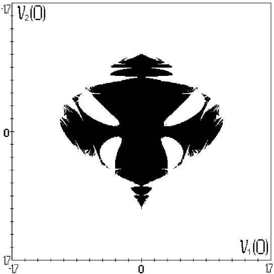
Figure 2: Stability diagram for the bush B$[a^{4},i]$ in the FPU-$\alpha$ chain.

In producing Fig. 2, we specify $\dot{\nu}_{1}(0)=0$, $\dot{\nu}_{2}(0)=0$, and change $\nu_{1}(0)$, $\nu_{2}(0)$ in some interval near their zero values. The stability domain, resembling a beetle, is drown in black color in the plain $\nu_{1}(0)$, $\nu_{2}(0)$. The bush B$[\hat{a}^{4},\hat{\imath}]$ losses its stability (and transforms into another bush of higher dimension), when we cross the boundary of the black region in any direction. From Fig. 2 it is obvious, how nontrivial stability domain for a bush of modes can be.

A detailed description of the stability domains for one-dimensional and two-dimensional bushes of modes in both FPU-$\alpha$ and FPU-$\beta$ chains can be found in FPU2 .

VI Conclusion

All the exact dynamical regimes in $N$-particle mechanical system with discrete symmetry can be classified by the subgroups $G_{j}$ of the parent group $G_{0}$, i.e. the symmetry group of its equations of motion. Actually, each subgroup $G_{j}$ singles out a certain invariant manifold which, being decomposed into the basis vectors of the irreducible representations of the group $G_{0}$, is termed as a “bush of modes” DAN1 ; DAN2 ; PhysD .

The bush B$[G_{j}]$, representing an $n$-dimensional vibrational regime, can be considered as a dynamical object characterized by its displacement pattern of all the particles from their equilibrium positions, by the appropriate dynamical equations and the domain of the stability. One-dimensional bushes are symmetry-determined similar nonlinear normal modes introduced by Rosenberg Ros (see also IntJ ). For Hamiltonian systems, the energy of the initial excitation turns out to be “trapped” in the bush and this is a phenomenon of energy localization in the modal space.

The different aspects of the bush theory were developed in DAN1 ; DAN2 ; PhysD ; IntJ ; ENOC ; C60 ; Octa . Bushes of vibrational modes (invariant manifolds) in the FPU chains were discussed in FPU1 ; FPU2 ; BR ; PR ; Shin .

The stability analysis of a given bush B$[G]$ reduces to studying the linearized (in the vicinity of the bush) dynamical equations $\ddot{\bm{\delta}}=\mathrm{J}(t)\cdot\bm{\delta}$. In the present paper, we prove (Theorem 1) that the symmetry group of the linearized system $\ddot{\bm{\delta}}=\mathrm{J}(t)\cdot\bm{\delta}$ turns out to be precisely the symmetry group $G$ of the considered bush B$[G]$. This result allows one to apply the well-known Wigner theorem about the specific structure of the matrix ($\mathrm{J}(t)$, in our case) commuting with all the matrices of a fixed representation (mechanical representation, in our case) of a given group. According to the above theorem one can split effectively the linearized system $\ddot{\bm{\delta}}=\mathrm{J}(t)\cdot\bm{\delta}$ into a number of independent subsystems of differential equations with time-dependent coefficients.

We want to emphasize that this symmetry-related method for splitting the linearized systems arising in the linear stability analysis of the dynamical regimes is suitable for arbitrary nonlinear mechanical systems with discrete symmetry. Such a decomposition (splitting) of the linearized system $\ddot{\bm{\delta}}=\mathrm{J}(t)\cdot\bm{\delta}$ is especially important for the multidimensional bushes of modes, describing quasiperiodic vibrational regimes, which cannot be treated with the aid of the Floquet method. Indeed, in this case, we need to integrate the differential equations with time-dependent coefficients over large time interval, unlike the case of periodic regimes where we can solve the appropriate differential equations over only one period to construct the monodromy matrix.

The above method is applied for studying the stability of some dynamical regimes (bushes of modes) in the monoatomic chains. For this specific mechanical systems, we prove Theorem 2 which allows one to find very simply the upper bound of dimensions of the independent subsystems obtained after splitting the linearized system $\ddot{\bm{\delta}}=\mathrm{J}(t)\cdot\bm{\delta}$. Indeed, according to this theorem, the dimension of each such subsystem does not exceed the integer $m$ determining the ratio of the volumes of the primitive cell of the chain in the vibrational state, corresponding to the given bush B$[G]=$B$[\hat{a}^{m},\dots]$, and the equilibrium state.

Taking into account any other symmetry elements of the considered bush allows to reduce the dimensions of at least some of the above discussed subsystems. We illustrate this fact comparing the stability analysis of the $\pi$-mode (zone boundary mode) for the FPU-$\alpha$ and FPU-$\beta$ chains.

- (1) V.P. Sakhnenko and G.M. Chechin, Dokl. Akad. Nauk 330, 308 (1993) [Phys. Dokl. 38, 219 (1993)];
- (2) V.P. Sakhnenko and G.M. Chechin, Dokl. Akad. Nauk 338, 42 (1994) [Phys. Dokl. 39, 625 (1994)].
- (3) G.M. Chechin and V.P. Sakhnenko, Physica D 117, 43 (1998).
- (4) G.M. Chechin, V.P. Sakhnenko, H.T. Stokes, A.D. Smith, and D.M. Hatch, Int. J. Non-Linear Mech. 35, 497 (2000).
- (5) G.M. Chechin, V.P. Sakhnenko, M.Yu. Zekhtser, H.T. Stokes, S. Carter, D.M. Hatch, in World Wide Web Proceedings of the Third ENOC Conference, http://www.midit.dtu.dk.
- (6) G.M. Chechin, O.A. Lavrova, V.P. Sakhnenko, H.T. Stokes, and D.M. Hatch, Fizika tverdogo tela 44, 554 (2002).
- (7) G.M. Chechin, A.V. Gnezdilov, and M.Yu. Zekhtser, Int. J. Non-Linear Mech. 38, 1451 (2003).
- (8) G.M. Chechin, N.V. Novikova, and A.A. Abramenko, Physica D 166, 208 (2002).
- (9) G.M. Chechin, D.S. Ryabov, and K.G. Zhukov, Physica D 203, 121 (2005).
- (10) P. Poggi, S. Ruffo, Physica D 103, 251 (1997).
- (11) B. Rink, Physica D 175, 31 (2003).
- (12) S. Shinohara, J. Phys. Soc. Japan 71, 1802 (2002); S. Shinohara, Progr. Theor. Phys. Suppl. 150, 423 (2003).
- (13) A. Cafarella, M. Leo, R. Leo, Phys. Rev. E 69, 046604 (2004).
- (14) K. Yoshimura, Phys. Rev. E 70, 016611 (2004).
- (15) T. Dauxois, R. Khomeriki, F. Piazza, S. Ruffo, Chaos, 15, 015110 (2005).
- (16) R.M. Rosenberg, J. Appl. Mech. 29, 7 (1962); R.M. Rosenberg, Adv. Appl. Mech. 9, 155 (1966).
- (17) J.P. Elliott, P.J. Dawber, Symmetry in Physics, Principles and Simple Applications, Macmillan, London, 1979.
- (18) N. Budinsky and T. Bountis, Physica D 8, 445 (1993).
- (19) K.V. Sandusky and J.B. Page, Phys. Rev. B 50, 866 (1994).
- (20) S. Flach, Physica D 91, 223 (1996).