Paraxial light in a Cole-Cole nonlocal medium: integrable regimes and singularities.

Abstract

Nonlocal nonlinear Schrödinger-type equation is derived as a model to describe paraxial light propagation in nonlinear media with different ‘degrees’ of nonlocality. High frequency limit of this equation is studied under specific assumptions of Cole-Cole dispersion law and a slow dependence along propagating direction. Phase equations are integrable and they correspond to dispersionless limit of Veselov-Novikov hierarchy. Analysis of compatibility among intensity law (dependence of intensity on the refractive index) and high frequency limit of Poynting vector conservation law reveals the existence of singular wavefronts. It is shown that beams features depend critically on the orientation properties of quasiconformal mappings of the plane. Another class of wavefronts, whatever is intensity law, is provided by harmonic minimal surfaces. Illustrative example is given by helicoid surface. Compatibility with first and third degree nonlocal perturbations and explicit solutions are also discussed.

PACS numbers: 02.30.Ik, 42.15.Dp

1 Introduction.

Propagation of the light through spatially nonlocal media is one of main subjects in modern nonlinear optics[(1), (2), (3), (4), (5), (6)]. Recently, it has been shown, both theoretically[(3)] and experimentally[(4), (5)], that highly nonlocal Kerr-type media supports propagation of stable laser beams, usually referred to as “solitons”. Laser beams propagating in Kerr-type media are modelled by the celebrated ($2+1$)D nonlinear Schrödinger (NLS) equation. Unlike ($1+1$)D NLS equation, it is not integrable by inverse scattering method[(7)]. In the case of high nonlocal media, (2+1)D NLS equation can be approximated by quantum harmonic oscillator (QHO) equation. Using results concerning QHO in the optics context, it has been possible to show the existence of solitons[(3)]. Nevertheless, a complete understanding of the rôle played by spatial nonlocal effects in the propagation of radiation in nonlinear media is still an open problem. Hence, it is of interest to investigate possible integrable regimes for three-dimensional nonlinear models.

In the present paper, we propose the nonlocal nonlinear Schrödinger-type (NNLS) equation as the model to describe a beam propagating in a medium with a certain spatial nonlocality degree and obeying some intensity law. By “intensity law” we mean certain functional dependence among dielectric function and intensity of the beam. We study the high frequency limit under specific assumptions, namely, the Cole-Cole dispersion law for the medium and suitably slow variation of the fields along propagating direction. Separating behaviors on the transverse and propagating directions, we derive two couples of equations for the phase and the intensity. Due to the intensity law, phase and intensity equations are strongly coupled and their compatibility appears to be a highly nontrivial problem.

As far as phase equations concerned, the compatibility has been studied in the papers [8; 9]. It has been shown that compatibility condition corresponds to the request that refractive index satisfies an infinite set of integrable equations referred to as dispersionless Veselov-Novikov (dVN) hierarchy. In particular, degrees of spatial nonlocality are in one-to-one correspondence with the orders of equations of dVN hierarchy.

So, we study compatibility among phase and intensity equations for certain assigned intensity law. We focus first on transverse equations. Their compatibility leads us to the study of a second order nonlinear partial differential equation. Since for most of physical models it satisfies the ellipticity condition we restrict ourselves to the class of so-called elliptic intensity laws.

The use of known results in the theory of elliptic equations and the special properties of Beltrami equation allows us to conclude that, for a generic elliptic intensity law, there exists singular wavefronts which can be used to describe self-guided beams. Moreover, we demonstrate that harmonic minimal surfaces provide us with a class of wavefronts for any elliptic intensity law. As explicit examples, helicoidal wavefronts are discussed. We stress that the helicoid is a well known example of singular wavefront which possesses several interesting propertiesBryngdahl ; Berry ; Vaughan ; Baranova ; Coullet ; Soskin1 ; Soskin2 . We show that helicoidal wavefronts are preserved for a specific class of first degree nonlocal perturbations up to next-to-leading order contributions. We present a simple example where the first degree nonlocality is responsible of a slight stretching or compression of the helicoid’s pitch.

General problem of compatibility among equations for transverse and propagating direction is difficult as much as crucial. In our model the consideration of propagating direction contributions is equivalent to inclusion of nonlocal terms. Besides, in the local case, equations for propagating direction are automatically compatible for any intensity law and it is sufficient to consider the transverse equations. We demonstrate that there exists a class of solutions for the third degree nonlocality which are in agreement with a suitable intensity law. Exploiting hydrodynamic-type reductions, found in the paper [17], we present some explicit formulae.

The paper is organized as follows: in section 2 derivation of nonlocal nonlinear Schrödinger equation is presented. In the section 3 phase equations and high frequency limit of Poynting vector conservation law in a Cole-Cole medium are displayed. A study of compatibility among intensity law and transverse equations and properties of solutions is presented in the section 4. Compatibility of intensity law and nonlocal perturbations is illustrated in section 5 by an explicit example. Some concluding remarks close the paper.

2 Nonlocal NLS-type equation.

Let us consider the nonlinear Maxwell equations

$$\begin{aligned} \nabla\wedge{\bf E}+\frac{\partial{\bf B}}{\partial t}&=0\quad{}\quad{}\nabla\cdot{\bf D}=0\\ \nabla\wedge{\bf B}-\frac{\partial{\bf D}}{\partial t}&=0\quad{}\quad{}\nabla\cdot{\bf B}=0\end{aligned}$$ (1)

where the displacement vector ${\bf D}={\bf D}({\bf E})$ depends nonlinearly on the electric field. We look for time-oscillating solutions such that

$${\bf E}\left({\bf x},t\right)={\bf E}\left({\bf x}\right)e^{-i\omega t},\quad{}{\bf D}\left({\bf x},t\right)={\bf D}\left({\bf x}\right)e^{-i\omega t}.$$

Under these assumptions one gets the following second order equationBorn

$$\nabla^{2}{\bf E}+\omega^{2}{\bf D}-\nabla\left(\nabla\cdot{\bf E}\right)=0.$$ (2)

Displacement vector ${\bf D}$ is chosen in a way to collect both nonlinear and nonlocal effects, i.e.

$${\bf D}=\varepsilon{\bf E}+{\bf F}_{NLoc}.$$ (3)

First term of the r.h.s. contains the nonlinearity. Dielectric function $\varepsilon$ is assumed to contain a weakly nonlinear perturbation of the form

$$\varepsilon=\varepsilon_{0}+\alpha^{2}\tilde{\varepsilon},\quad{}\alpha<<1,$$ (4)

where $\tilde{\varepsilon}$ depends on the intensity of the radiation.

The second term in the r.h.s. of (3) provides us with the spatial nonlocal response of the medium. We assume it to be of the form

$${\bf F}_{NLoc}=\alpha\left(\sum_{n=1}^{3}c_{n}\frac{\partial{\bf E}}{\partial x_{n}}+\sum_{l,m=1}^{3}c_{lm}\frac{\partial^{2}{\bf E}}{\partial x_{l}~{}\partial x_{m}}+\dots\right).$$ (5)

One gets the expression (5) for the nonlocal term considering an integral relation among the displacement and the electric field where the kernel is a sum of $\delta$-functions and spatial derivatives. We define the degree of nonlocality as the maximum derivative order which appears in expression (5).

Paraxial approximation is performed according to the rule (see e.g. Ref. 19)

$${\bf E}\rightarrow\alpha{\bf E}e^{ikz}\quad{}{\bf D}\rightarrow\alpha{\bf D}e^{ikz}$$ (6)

(setting vacuum light speed $c=1$, $k=\sqrt{\varepsilon_{0}}\omega$), and the amplitudes are assumed to depend slowly on the coordinates in such a way that the gradient acts as follows

$$\nabla=\left(\frac{\partial}{\partial x},\frac{\partial}{\partial y},\frac{\partial}{\partial z}\right)\rightarrow\left(\alpha\nabla_{\bot},\alpha^{2}\frac{\partial}{\partial z}\right).$$ (7)

Using the expression (3) and the rules (6) and (7) in the second order equation (2), one shows that the first nontrivial contribution is of the order ${\cal O}\left(\alpha^{3}\right)$ and it provides us with the nonlocal nonlinear Schrödinger-type (NNLS) equation

$$2i\sqrt{\varepsilon_{0}}\omega\frac{\partial{\bf E}}{\partial z}+\nabla_{\bot}^{2}{\bf E}+\omega^{2}\tilde{\varepsilon}{\bf E}+{\cal F}_{NLoc}=0$$ (8)

where

$$F_{NLoc}={\cal F}_{NLoc}+{\cal O}\left(\alpha^{4}\right).$$ (9)

Note that in absence of nonlocal contribution ${\cal F}_{NLoc}$ and for a Kerr type nonlinear response of the medium, equation (8) becomes the standard nonlinear Schrödinger equation in $2+1-$dimensions.

3 Geometrical optics limit of NNLS equation in Cole-Cole media.

In this section we study the geometrical optics limit of NNLS equation for a medium which satisfies so-called Cole-Cole dispersion lawColeCole

$$\tilde{\varepsilon}=\tilde{\varepsilon}_{0}+\frac{\tilde{\varepsilon}_{1}}{1+(i\tau_{0}\omega)^{2\nu}},\quad 0<\nu<\frac{1}{2},$$ (10)

where $\tau_{0}$ is the relaxation time and $\nu$ is a suitable phenomenological exponent whose range of values is of crucial importance in the following derivations. Relation (10) describes frequency dependence of dielectric function for several polar media as well as liquid crystals and various biological tissues (see e.g. Refs. [20; 21]).

We study a particular high frequency regime of NNLS equation where the phase of electric field varies slowly along $z$-direction in such a way that

$$z\rightarrow\omega^{2\nu}z,\quad{}\frac{\partial}{\partial z}\rightarrow\omega^{-2\nu}\frac{\partial}{\partial z}.$$ (11)

We also assume nonlocal effects to be weak in high frequency limit in such a way that they contribute at most with $\omega^{-2\nu}-$order terms

$${\cal F}_{NLoc}=\omega^{-2\nu}\tilde{{\cal F}}_{NLoc}+{\cal O}\left(\omega^{-4\nu}\right)$$ (12)

In order to calculate geometrical optics limit we adopt, as usual, the following representation of electric field

$${\bf E}={\bf f}(x,y,\omega^{2\nu})\ e^{i\omega S(x,y,\omega^{2\nu}z)}.$$ (13)

Expansion of all functions with respect to small parameter $\omega^{-2\nu}$

together with dispersion law (10) and the prescriptions (11) leads us to the high frequency limit of NNLS equation at the orders $\omega^{2}$ and $\omega^{2-2\nu}$:

$$\left(\nabla_{\bot}S\right)^{2} =4u,$$ (14a)

$$S_{z} =\varphi(S_{x},S_{y},x,y,z)$$ (14b)

where $4u=\tilde{\varepsilon}_{0}$ and $\varphi=\left(\tilde{\varepsilon}_{1}+\tilde{{\cal F}}_{NLoc}\right)/\left(2\sqrt{\varepsilon_{0}}\right)$. For convenience we denote the partial derivative of a function $f$ with respect to variable $\eta$ as $f_{\eta}$. We stress that condition on the exponent $0<\nu<1/2$ is crucial to separate equation (14b) from polarization contributions. Equation (14a) is the standard eikonal equation in two-dimensions while the function $\varphi$ in equation (14b) is an $N$-degree polynomial in $S_{x}$ and $S_{y}$ and it describes an $N$-degree nonlocal response. Moreover, in agreement with inversion phase symmetry ($S\to-S$) of the eikonal equation, polynomial degree of function $\varphi$ must be odd. We note also that the system of equations (14) has been derived first directly from the Maxwell equationsMoro2 . In the present paper, we will consider local response and first and third degree nonlocal responses.

In local case we have

$$\varphi=\varphi(z),\quad{}u=u(x,y),$$ (15)

where $\varphi$ and $u$ are certain function of their arguments. For a first degree nonlocality we have

$$\varphi=\alpha_{1}S_{x}+\alpha_{2}S_{y},\quad{}$$ (16)

and $u$ must satisfy the following linear equation

$$u_{z}=\left(\alpha_{1}u\right)_{x}+\left(\alpha_{2}u\right)_{y}$$ (17)

where $\alpha_{1}$ and $\alpha_{2}$ are harmonic conjugate functions (they satisfy Cauchy-Riemann conditions $\alpha_{1x}=\alpha_{2y}$ and $\alpha_{1y}=-\alpha_{2x}$). Finally, for a third degree nonlocal response we have

$$\varphi=\frac{1}{4}S_{x}^{3}-\frac{3}{4}S_{x}S_{y}^{2}+V_{1}S_{x}+V_{2}S_{y}$$ (18)

and $u$ satisfies the dispersionless Veselov-Novikov equation

$$\begin{aligned} &u_{z}=\left(V_{1}u\right)_{x}+\left(V_{2}u\right),\\ &V_{1x}-V_{2y}=-3u_{x},\\ &V_{1y}+V_{2x}=3u_{y}.\end{aligned}$$ (19)

In order to complete geometrical optics description we construct high frequency limit of Poynting vector conservation law

$$\nabla\cdot{\bf P}=0.$$ (20)

Poynting vector can be written down as follows

$${\bf P}=I\frac{\nabla S^{\ast}}{\left|\nabla S^{\ast}\right|}$$ (21)

where

$$S^{\ast}=\sqrt{\varepsilon}_{0}z+S(x,y,\omega^{2\nu}z)$$ (22)

is the total phase of electric field and $I$ is the intensity. In the following, for sake of simplicity, we set dielectric constant $\varepsilon_{0}=1$. Using the previous prescriptions to perform high frequency limit in paraxial approximation and expanding intensity

$$I=I_{0}+\omega^{-2\nu}I_{1},$$ (23)

one concludes that equation (20) leads to the following set of equations for $I_{0}$ and $I_{1}$

$$\nabla_{\bot}I_{0}\cdot\nabla_{\bot}S+I_{0}\nabla_{\bot}^{2}S =0$$ (24a)

$$\nabla_{\bot}I_{1}\cdot\nabla_{\bot}S+I_{1}\nabla_{\bot}^{2}S+\frac{\partial I_{0}}{\partial z} =0.$$ (24b)

In this regime, properties of the light are completely described by the systems of equations (14) and (24). If no additional conditions are considered, once compatibility of equations (14) is guaranteed, linear system (24) provides us with leading orders intensity contributions $I_{0}$ and $I_{1}$.

Integrability of the phase equations (14) has been discussed in details in Refs. [8; 9]. In particular, it has been shown that for a function $\varphi$ with a polynomial dependence on $S_{x}$ and $S_{y}$, compatibility condition of equations (14) selects the class of refractive indices which satisfy the dispersionless limit of the Veselov-Novikov (dVN) hierarchy. In particular, dVN hierarchy allows us to classify different degrees of nonlocal response by a one-to-one correspondence among degrees of the polynomials $\varphi$ and the equations of the hierarchy.

We mention that dVN hierarchy is amenable by the quasiclassical $\bar{\partial}$-dressing methodMoro2 and a reduction method based on symmetry constraints appears to be an effective method to construct exact solutionsBogdanov .

4 Phase and intensity transverse equations.

4.1 Elliptic intensity law.

Several models in nonlinear optics analyze a self-action of the medium assuming that the influence of an external electromagnetic field is described by a functional dependence among intensity and refractive index $I=I(u)$. This is the form of intensity law in the geometrical optics limit. Kerr type media, where $I\propto u$, and saturable nonlinear media such that $u\propto\log(1+I/I_{t})$, where $I_{t}$ is the so-called threshold intensity, are two famous examples. Of course, for self-action nonlinear media models phase equations (14) and intensity equations (24) appear to be strongly coupled and the study of their compatibility is a highly non-trivial problem. In the present section, we analyze compatibility and properties of equations (14a) and (24a), here referred to as transverse equations. We note that this analysis is quite trivial in the case of the media exhibiting local response. Indeed, according to relations (15) $u$ does not depend on the $z$-variable. Then, equation (24b) coincides with equation (24a) and they are automatically compatible with (14b).

Let us consider a self-action nonlinear medium obeying intensity law $I_{0}=I_{0}(u)$. Observing that $\nabla_{\bot}I_{0}=I_{0}^{\prime}\nabla_{\bot}u$, where “prime” means the derivative with respect its argument $u$, and using equation (14a) in (24a), one gets the following second order partial differential equation

$$AS_{xx}+BS_{yy}+2CS_{xy}=0,$$ (25)

where by definition ${\cal I}_{0}=\log I_{0}$ and

$$A={\cal I}_{0}\;^{\prime}S_{x}^{2}+2,\quad{}B={\cal I}_{0}\;^{\prime}S_{y}^{2}+2,\quad{}C={\cal I}_{0}\;^{\prime}S_{x}S_{y}.$$ (26)

Recall that properties of a second order partial differential equation depend critically on the discriminant

$$\Delta=AB-C^{2}.$$ (27)

If $A>0$, equation is of the elliptic type when $\Delta>0$ , parabolic when $\Delta=0$ and hyperbolic when $\Delta<0$. In this paper we focus on the elliptic case motivated by the fact that a wide class of such models for optical spatial solitons is provided by a Kerr dependence or logarithmic saturable nonlinearities. Indeed, one can simply verify that for a Kerr-type intensity law of the form $I=u^{\beta}$ where $\beta>0$ and a logarithmic one, $u=\log(1+I_{0}/I_{0,t})$, one has $\Delta=4(2{\cal I}_{0}\;^{\prime}u+1)>0$ uniformly. Ellipticity of equation (25) seems to be associated to important physical properties of a wide class of nonlinear media. Moreover, elliptic equations such as (25) have been well studied in mathematics and possess several remarkable analytical and geometrical propertiesBojarski ; Iwaniec ; Bers ; Vekua ; Ahlfors ; Lehto .

Now, we will study equation (25). Introducing complex variable $\lambda=x+iy$ and the complex gradient $w=S_{x}-iS_{y}$, one can rewrite equation (25) equivalently as follows

$$aw_{\lambda}+bw_{\bar{\lambda}}+\bar{a}\bar{w}_{\bar{\lambda}}+\bar{b}\bar{w}_{\lambda}=0,$$ (28)

where

$$a=\frac{1}{2}\left(A-B+2iC\right),\quad{}b=\frac{1}{2}\left(A+B-2iC\right).$$ (29)

A class of solutions of equation (28) is provided by the solutions of, the so-called, nonlinear Beltrami equation

$$w_{\bar{\lambda}}=\mu\left(w,\bar{w}\right)w_{\lambda},\quad{}\mu=-\frac{a}{b}.$$ (30)

It is straightforward to verify that ellipticity condition $\Delta>0$ implies $\left|\mu\right|<1$. Beltrami equation describes so-called quasiconformal mapping of the plane of complex dilatation $\mu$Ahlfors ; Lehto . This fact highlights an intriguing connection among geometrical optics and quasiconformal mapping theory.

For instance, let us consider a laser beam whose input profile is $I_{0}\neq 0$ inside a simply connected domain $G$ and $I_{0}=0$ on the smooth boundary $\Gamma$ of $G$ and outside it. Because of functional relation $I_{0}=I_{0}(u)$, refractive index is constant on $\Gamma$ too. More specifically, we have

$$w(\lambda)\bar{w}(\lambda)=4u_{0},\quad{}\lambda\in\Gamma.$$ (31)

Boundary $\Gamma$ is mapped on the $2\sqrt{u_{0}}$-radius circle. In virtue of equation (31), for $\lambda\in\Gamma$ one can write $w=2\sqrt{u_{0}}\exp(i\theta)$. Then, if $w$ is assigned in such a way that, for instance, $w(0)=0$, where $0\in G$ is assumed, variation of argument of complex number $w$ is

$$\mathop{\rm\Delta}\limits_{\Gamma}\arg w=2\pi.$$

Under mentioned conditions, it can be demonstrated that $w$ is a homeomorphic mapping of domain $G$ onto $2\sqrt{u_{0}}-$radius disk $\Gamma\;^{\prime}$Iwaniec . As a consequence, mapping $w$ preserve the topology of domain $G$. It could be interesting to note that if $w=w(\lambda,z)$ “evolves” along $z$ according to equation (14b) and this evolution is compatible with equation (25), inverse mapping (it exists since $w$ is homeomorphic) $\lambda=\lambda(w)$, with $w\in\Gamma\;^{\prime}$, provides us with the beam profile at any $z$.

Mapping $w=S_{x}-iS_{y}=\left(S_{x},-S_{y}\right)$ can be also regarded as a two-dimensional vector field on the $\lambda-$plane associated with transverse components of the wavefront normal unit vector. In the case $\varphi\equiv 0$, it is has the simple form

$${\bf n}=\frac{\nabla S^{\ast}}{\left|\nabla S^{\ast}\right|}=\left(\frac{S_{x}}{\sqrt{1+4u}},\frac{S_{y}}{\sqrt{1+4u}},\frac{1}{\sqrt{1+4u}}\right).$$ (32)

From this point of view, mapping $w$ gives us information about light-rays distribution around propagating direction.

As specific example, let us consider a mapping as in figure 1a. Curves $\Gamma$ and $\Gamma^{\prime}$ are oriented leaving domain on the right hand side. Under conditions mentioned above, there exists a homeomorphism $w$ of domain $G$ onto $G^{\prime}$ acting in such a way that $w(s_{1},0)=(-1,0)$, $w(0,s_{2})=(0,1)$ and $w(-s_{3},0)=(1,0)$. Consequently, normal unit vector to wave-front on the boundary $\Gamma$ points inside the domain $G$ (recall that $y$-component of $w$ reverse $y$-component of $\bf{n}$). This mapping allows the radiation to be ‘self-guided’ around propagating direction. Conversely, if $w(s_{1},0)=(1,0)$, $w(0,s_{2})=(0,-1)$ and $w(-s_{3},0)=(0,-1)$ radiation spreads transversely far from $z-$axis. Note that in both cases homeomorphism $w$ is sense-reversing. If we consider a sense-preserving mapping such as, for instance, $w(s_{1},0)=(1,0)$, $w(0,s_{2})=(0,1)$ and $w(-s_{3},0)=(-1,0)$, the beam spreads along $x-$direction and tends to be trapped along $y-$axis (see figure 1b). We emphasize, finally, that all of these observations can be generalized to the case of arbitrary $n-$connected domains.

Figure 1: a) Sense-reversing mappings describe beams which tend to be trapped (solid line) or spread (dashed line). b) If the mapping is sense-preserving light beam spreads along $x-$direction and tends to be trapped along $y-$direction.

Another class of solutions of equation (28) can be obtained solving the equation

$$bw_{\bar{\lambda}}+\bar{a}\bar{w}_{\bar{\lambda}}=0.$$ (33)

Passing to reciprocal coordinates by inversion of the system

$$\begin{aligned} \lambda&=\lambda(w,\bar{w})\\ \bar{\lambda}&=\bar{\lambda}(w,\bar{w}),\end{aligned}$$ (34)

one converts equation (33) into the form of the linear Beltrami equation

$$\lambda_{\bar{w}}=\nu(w,\bar{w})\lambda_{w},$$ (35)

where $\nu(w,\bar{w})=\bar{a}/b$ and, due to ellipticity, $|\nu|<1$. The advantage of the use of the reciprocal transformation is that the Beltrami equation is just linear and several properties of the analytic functions can be rigorously generalized to its solutions (see e.g. Ref. [25]). An interesting result is provided by the generalization of Liouville theorem. Indeed, if $\lambda=\lambda(w,\bar{w})$ is bounded on whole $w-$plane and satisfies linear Beltrami equation (35) it can be shown (Vekua’s theorem) that $\lambda(w,\bar{w})\equiv\textup{constant}$VekuaTh . Of course, for the constant solution, mapping from $w-$to$-\lambda-$plane is singular and reciprocal transformation (34) is not defined. Then, any non-trivial solution of equation (35) must be singular somewhere on the complex plane and different type of singularities can occur, such as poles, essential singularities, singularities of the derivatives etc. A complete analytical and geometrical classification of them will be done elsewhere InPreparation .

For sake of simplicity, let us consider a solution $\lambda(w,\bar{w})$ having a simple pole at $w=0$. As discussed above, one can always consider a homeomorphism from $D^{\prime}=\mathbb{C}\setminus D_{\epsilon}$ to $D_{R}$ where $D_{\epsilon}$ is a disk of arbitrarily small radius $\epsilon$ on the $w-$plane and $D_{R}$ is the $R$-radius disk on the $\lambda-$plane, mapping the boundary of $D_{\epsilon}$ on the boundary of $D_{R}$. Inverse mapping $w:\;D_{R}\to D^{\prime}$ constructed in such a way can be used to describe a beam “confined”around $z-$axis. Indeed, light rays crossing the boundary of $D_{R}$ can settled down arbitrarily parallel to $z-$axis as much as disk $D_{\epsilon}$ is small.

Coming back to nonlinear Beltrami equation (30), we expect that for “mild enough” complex dilatations $\mu$, Vekua’s theorem still holds. In these cases, the only one bounded solution on whole $\lambda-$plane is $w=\textup{constant}$. In most of meaningful physical situations, intensity distribution on the $\lambda-$plane, at certain $z$, goes to zero for $\lambda\to\infty$, or equivalently, one can says that intensity vanishes outside a big enough $R-$radius disk $D_{R}$. Thus, outside $D_{R}$, refractive index assumes a constant value $u=u_{0}$ and the solutions of eikonal equation (14a) is

$$S=c_{0}x+c_{1}y+c_{3},$$ (36)

where $c_{0}$, $c_{1}$ and $c_{3}$ are constants and the condition $c_{0}^{2}+c_{1}^{2}=4u_{0}$ holds. For a paraxial beam we have $c_{0}=c_{1}=0$. By a consequence $w=S_{x}-iS_{y}=c_{0}-ic_{1}=0$ and, of course it satisfies Beltrami equation in $\mathbb{C}\setminus D_{R}$. In virtue of Vekua’s theorem, the only one bounded solution is $w\equiv 0$. Then, any non-trivial solution must be singular somewhere on the plane. In our example, wavefront is approximately plane for $\lambda\in\mathbb{C}\setminus D_{R}$ and possesses singularity inside $D_{R}$.

4.2 Minimal surfaces: the helicoid example.

Standard approach to calculate solutions of Beltrami equation is based on its reduction to a two-dimensional integral equation Vekua ; Tricomi which is amenable by using the successive approximation method. In general, to find ‘explicit’ exact solutions is a quite challenging problem and successful chances are critically depending on the form of the complex dilatation. Incidentally, we note that solutions possessing cylindrical symmetry such that

$$S=S(r),\quad{}u=u(r),\quad{}r=\sqrt{x^{2}+y^{2}},$$ (37)

are not compatible with intensity law. It is straightforward to verify that equations (14a) and (24a) along with assumptions (37) imply that intensity depends explicitly on $z-$axis distance $r$

$$I_{0}=\frac{1}{2cr\sqrt{u}},$$ (38)

where $c$ is an arbitrary constant.

Here, we discuss solution of the equation (25) in connection with the minimal surfaces. They are described by the following elliptic equation (see e.g. Ref. 31)

$$\left(1+S_{y}^{2}\right)S_{xx}+\left(1+S_{x}^{2}\right)S_{yy}-2S_{x}S_{y}S_{xy}=0.$$ (39)

Now, we restrict ourselves to the class of solutions of equation (25) which are also harmonic, that is

$$S_{xx}+S_{yy}=0.$$ (40)

Using condition (40) in equation (25), one gets the equation

$$S_{x}^{2}S_{xx}+S_{y}^{2}S_{yy}+2S_{x}S_{y}S_{xy}=0,$$ (41)

for any intensity law. It is straightforward to check that equations (41) and (39) coincide for harmonic solutions. In other words, a class of solutions of equation (25), whatever is dependence $I_{0}=I_{0}(u)$, is just given by the class of the harmonic minimal surfaces. An interesting non-trivial example of solution is

$$S=K\arctan\left(\frac{y}{x}\right),$$ (42)

where $K$ is an arbitrary constant. It is straightforward to check that function $S$ in (42) satisfies equations (39), (40) and (41) simultaneously. Equation of corresponding wavefronts is

$$S^{\ast}\equiv z+K\arctan\left(\frac{y}{x}\right)=\textup{const},$$ (43)

where the constant $K$ is the “pitch” of the helicoid. We stress that singular wavefronts of the form (43) are well known in the theory of nonlinear singular optics and their topological properties have important phenomenological consequences connected with description of screw wavefront dislocations or so-called optical vorticesVaughan ; Baranova ; Coullet (see also Ref. [15,16] and references therein). Note that complex gradient associated with the helicoid

$$w=-i\frac{K}{\lambda}$$ (44)

is analytic and it has a simple pole singularity at $\lambda=0$. Nevertheless, normal vector to the wavefront, whose components coincides (up to a sign) with real and imaginary parts of $w$, is not defined. Indeed, vector $w=(S_{x},-S_{y})$ has no limit as $\left(x,y\right)\to 0$. Figure 2 shows examples of helicoidal wavefronts (43) usually parametrized as follows

$$x=v\cos t,\quad{}y=v\sin t,\quad{}z=Kt.$$ (45)

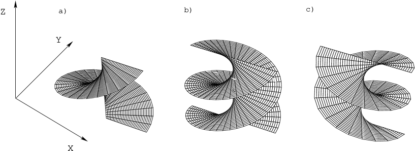
Figure 2: Helicoidal structures of wavefront around $z-$axis: a) one-start right-screw ($K=1$); b) two-start right screw ($K=1$); c) two-start left screw ($K=-1$).

One-started helicoid shown in figure 2a is obtained for $0<v<+\infty$; two-started helicoids shown in figure 2b,c are obtained for $-\infty<v<+\infty$. Refractive index

$$u=\frac{K^{2}}{4(x^{2}+y^{2})}$$ (46)

has cylindrical symmetry around $z-$axis and displays divergence at $\lambda=0$. Thus, in most of physical cases one has a divergence of intensity $I_{0}$. This means that around $\lambda=0$ geometrical optics approximation fails and wave effects become relevant. In particular, necessary condition for the existence of singular wavefronts is that intensity vanishes where phase function is singular. Indeed, in this region interference phenomenon is no more negligible and can realize this condition.

Finally, we note that helicoidal wavefront is ‘stable’, up to $\omega^{-2\nu}-$orders deformations, for a specific class of first degree nonlocal perturbations. In this case, the phase (42) is defined up to an additive arbitrary function of $z-$variable $\psi(z)$, such that $\psi^{\prime}=\varphi(z)$. Thus, using the phase expression $S=K\arctan\left(y/x\right)+\psi(z)$ along with relation (46) in equations (16) and (17), we conclude that the helicoid is deformed for nonlocal harmonic data $\alpha_{1}$ and $\alpha_{2}$ satisfying simultaneously the following equations

$$\begin{aligned} \left(x^{2}+y^{2}\right)\alpha_{1x}&=x\alpha_{1}+y\alpha_{2}\\ -y\alpha_{1}+x\alpha_{2}&=\varphi(z)\left(x^{2}+y^{2}\right).\end{aligned}$$ (47)

Trivial solutions $\alpha_{1}=\alpha_{2}=\varphi=0$ corresponds to the local case discussed above. A simple non-trivial solution $\alpha_{1}=-\gamma y$, $\alpha_{2}=\gamma x$ and $\varphi=\gamma$, where $\gamma$ is an arbitrary constant, provides us with the following wavefront (we remind that to return to speed variables one has to substitute $\psi(z)\to\psi(\omega^{-2\nu}z)$)

$$S^{\ast}\equiv z+\frac{K}{1+\omega^{-2\nu}\gamma}\arctan\left(\frac{y}{x}\right)=\textup{const}.$$ (48)

Note that for $\gamma=0$ equation (48) coincides with the equation (43). As a consequence of nonlocal response the helicoid’s pitch is compressed if $\gamma>0$ and stretched if $\gamma<0$.

5 Intensity law and nonlocal perturbations.

Compatibility condition between dVN hierarchy and the intensity law $I_{0}=I_{0}(u)$ is an as challenging as intriguing issue. Indeed, due to the Beltrami equation, it could establish a direct connection between dispersionless integrable systems and an entire class of quasiconformal functions parametrized by $z$. Unfortunately, intensity law appears to be quite restrictive making the problem of compatible nonlocal responses rather non-trivial one. This section is devoted to demonstration of the existence of a suitable intensity law such that systems (14) and (24) are compatible for a third degree nonlocal response.

To do that, we consider hydrodinamic type reductions of dVN equation. They have been found using symmetry constraint of the form $\nabla_{\bot}^{2}S=u_{x}$Bogdanov . It can be shown that dVN equation (19) is reduced to following hydrodynamic-type system

$$\left(\begin{array}[]{cc}p_{1}\\ p_{2}\\ \end{array}\right)_{y} =\left(\begin{array}[]{cccc}0&1\\ 2p_{1}-1&2p_{2}\\ \end{array}\right)\left(\begin{array}[]{cc}p_{1}\\ p_{2}\\ \end{array}\right)_{x}$$ (55)

$$\left(\begin{array}[]{cc}p_{1}\\ p_{2}\\ \end{array}\right)_{z} =\left(\begin{array}[]{cc}A_{11}&A_{12}\\ A_{21}&A_{22}\\ \end{array}\right)\left(\begin{array}[]{cc}p_{1}\\ p_{2}\\ \end{array}\right)_{x}$$ (62)

where

$$A_{11}=3p_{1}\left(p_{1}-1\right) A_{12}=3p_{2},$$

$$A_{21}=3p_{2}\left(2p_{1}-1\right) A_{22}=3p_{1}\left(p_{1}-1\right)+6p_{2}^{2}$$

and $p_{1}:=S_{x}$, $p_{2}:=S_{y}$.

Now, looking for solutions such that $p_{2}=p_{2}(p_{1})$, $p_{1}$ and $p_{2}$ are given in implicit form in terms of the following algebraic system

$$x+G^{\prime}y+H^{\prime}z-\Phi\left(p_{1}\right)=0$$ (63)

$$p_{2}=\frac{1}{2}\left[\xi+\frac{2c-\log\left(\xi+\sqrt{1+\xi^{2}}\right)}{\sqrt{1+\xi^{2}}}\right]$$ (64)

$$\xi=p_{2}\pm\sqrt{p_{2}^{2}+2p_{1}-1}$$

where $c$ is an arbitrary constant, $G=p_{2}(p_{1})$, $H=p_{1}^{3}-\frac{3}{2}p_{1}^{2}+\frac{3}{2}p_{2}^{2}(p_{1})$ and ‘prime’ means the derivative with respect to $p_{1}$.

Differentiating eikonal equation (14a) with respect to $x$ and taking into account that $u_{x}=\nabla_{\bot}^{2}S$, one gets

$$\nabla_{\bot}\left(-\frac{S_{x}}{2}\right)\cdot\nabla_{\bot}S+\nabla_{\bot}^{2}S=0.$$ (65)

Comparing equation (65) with intensity equation (24a), one obtains the following nice relation among intensity and $p_{1}-$component of the gradient

$$I_{0}=C\;e^{-\frac{p_{1}}{2}},$$ (66)

where $C$ is an arbitrary real constant. Finally, eikonal equation provides us with intensity law

$$u(I_{0})=\left(\log\frac{I_{0}}{C}\right)^{2}+\frac{1}{4}\left[p_{2}\left(-2\log\frac{I_{0}}{C}\right)\right]^{2},$$ (67)

where last term in r.h.s. is given by algebraic relation (64).

6 Conclusions.

NNLS equation (8) has been proposed as the generalization of NLS equation in order to include different degrees of nonlocal responses. Of course, just like (2+1)D NLS equation, NNLS equation is not integrable. Particular high frequency regimes discussed in this paper allows us to investigate interplay among a wide class of nonlinear responses and nonlocal perturbations free from interference effects. At leading order non-trivial wavefronts exhibit singular vortex-type behaviors. Moreover, singular phases can support propagation of self-guided beams. Harmonic elliptic surfaces provide also with stable beams with singular wavefronts such as the helicoid. Moreover, there exists special first degree nonlocal perturbations preserving helicoidal wavefronts. In the example considered, first degree nonlocal perturbation produces a stretching or compression of helicoid’s pitch. A classifications of singularities and their properties should provides us with a deeper understanding of this phenomena and seems to be a promising subject of study.

On the other hand it has been shown that intensity law is compatible with third degree nonlocal perturbations. In particular, we note that new hydrodynamic-type reductions, obtained by symmetry constraints approach can be very useful to calculate new compatible intensity laws. This will stimulates our efforts in that direction. Finally, we observe that although the class of solutions in nonlocal perturbation regimes appears to be not too large, example discussed above shows they are highly non-trivial. Hence, in this regime, interesting and unexpected phenomena could occur.

- (1) M. Segev, B. Crosignani and A. Yariv, “Spatial solitons in photorefractive media”, Phys. Rev. Lett., 68, pp. 923-926, 1992.
- (2) G. C. Duree et al., “Observation of self-trapping of an optical beam due to the photorefractive effect”, Phys. Rev. Lett., 71, pp. 533-536, 1993.
- (3) A. W. Snyder and D. J. Mitchell, “Accessible solitons”, Science, 276, pp. 1538-1541, 1997.
- (4) C. Conti, M. Peccianti and G. Assanto, “Route to nonlocality and observation of accessible solitons”, Phys. Rev. Lett., 91, pp. 0739011-0739014, 2003.
- (5) C. Conti, M. Peccianti and G. Assanto, “Observation of optical spatial solitons in a highly nonlocal medium”, Phys. Rev. Lett., 92, pp. 1139021-1139024, 2004.
- (6) For a review on optical spatial solitons: G. I. Stegeman and M. Segev, “Optical spatial solitons and their interactions: universality and diversity”, Science, 286, pp. 1518-1523, 1999.
- (7) M.J. Ablowitz and H. Segur, Solitons and the Inverse Scattering Transform, SIAM, Philadelphia, 1981.
- (8) B. Konopelchenko and A. Moro, “Geometrical optics in nonlinear media and integrable equations”, J. Phys. A: Math. Gen., 37, pp. L105-L111, 2004.
- (9) B. Konopelchenko and A. Moro, “Integrable equations in nonlinear geometrical optics”, Stud. Appl. Math., 113, pp. 325-352, 2004.
- (10) O. Bryngdahl, “Radial and circular fringe interferograms”, J. Opt. Soc. Am., 63, pp. 1098-1104, 1973.
- (11) J. F. Nye and M.V. Berry, “Dislocations in waves trains”, Proc. R. Soc. A, 336, pp. 165-190, 1974.
- (12) J. M. Vaughan and D. V. Willets, “Interference properties of a light beam having a helical wave surface”, Opt. Comm., 30, pp. 263-267, 1979.
- (13) N. B. Baranova et al., “Wavefront dislocations: topological limitations for adaptive systems with phase conjugation”, J. Opt. Soc. Am., 73, pp. 525-528, 1983.
- (14) P. Coullet, L. Gil and F. La Rocca, “Optical vortices”, Opt. Comm., 73, pp. 403-408, 1989.
- (15) I. V. Basistiy, M. S. Soskin, M. V. Vasnetsov, “Optical wavefront dislocations and their properties”, Opt. Comm., 119, pp. 604-612, 1995.
- (16) M. S. Soskin and M. V. Vasnetsov, “Nonlinear singular optics”, Pure Appl. Opt., 7, pp. 301-311, 1998.
- (17) L. Bogdanov, B. Konopelchenko and A. Moro, “Symmetry constraints for real dispersionless Veselov-Novikov equation”, Fund. Prikl. Mat., 10, pp. 5-15, 2004 (russian); english version to appear on J. Math. Sci.; preprint arXiv:nlin.SI/0406023, (2004).
- (18) M. Born and E. Wolf, Principles of Optics, p. 10, Pergamon Press, Oxford, 1980.
- (19) L.D. Landau, E.M. Lifshitz and L.P. Pitaevski, Electrodynamics of continuous media, vol. 8, Pergamon Press, Oxford, 1984.
- (20) K.S. Cole and R.H. Cole, “Dispersion and absorption in dielectrics”, J. Chem. Phys., 9, pp. 341-351, 1941.
- (21) Y. Kimura, S. Hara and R. Hayakawa, “Nonlinear dielectric relaxation spectroscopy of ferroelectric liquid crystals”, Phys. Rev. E, 62, pp. R5907-R5910-2000, ; D. Haemmerich, S.T. Staelin, J.Z. Tsai, S. Tungjitkusolmun, D.M. Mahvi and J.G. Webster, “In vivo electrical conductivity of hepatic tumours”, Physiol. Meas., 24, pp. 251-260, 2003.
- (22) B. Bojarski, “Quasiconformal mappings and general structural properties of systems of nonlinear equations elliptic in the sense of Lavrent’ev”, Symposia Mathematica, 18, pp. 485-499, 1976.
- (23) T. Iwaniec, “Quasiconformal mapping problem for general nonlinear systems of partial differential equations”, Symposia Mathematica, 18, pp. 501-517, 1976.
- (24) L. Bers, “Quasiconformal mappings with applications to differential equations, function theory and topology”, Bull. Am. Math. Soc., 83, pp. 1083-1100, 1977.
- (25) I.N. Vekua, Generalized Analytic functions, Pergamon, Oxford, 1962.
- (26) L.V. Ahlfors, Lectures on quasi-conformal mappings, D. Van Nostrand C., Princeton, 1966.
- (27) O. Lehto and K.I. Virtanen, Quasi-conformal mappings in the plane, Springer-Verlag, Berlin, 1973.
- (28) See theorem 3.32 p. 213 in Ref. 25.
- (29) B. Konopelchenko and A. Moro, in preparation.
- (30) F. Tricomi, “Equazioni integrali contenenti il valor principale di un integrale doppio”, Math. Ztschr, 27, pp. 87-133, 1928.
- (31) B. A. Dubrovin, A.T. Fomenko and S. P. Novikov, Modern geometry-Methods and applications. Part I. The geometry of surfaces, transformation groups and fields, Springer, New York, 1984.