Optimal phase space projection for noise reduction

Abstract

In this communication we will re-examine the widely studied technique of phase space projection. By imposing a time domain constraint (TDC) on the residual noise, we deduce a more general version of the optimal projector, which includes those appearing in previous literature as subcases but does not assume the independence between the clean signal and the noise. As an application, we will apply this technique for noise reduction. Numerical results show that our algorithm has succeeded in augmenting the signal-to-noise ratio (SNR) for simulated data from the Rössler system and experimental speech record.

I Introduction

Due to its simplicity in implementation and efficiency in computation, noise reduction based on phase space projection has been widely studied in previous literature. For example, Broomhead and King broomhead extracting (2) advocated that, in case of white noise, via singular value decomposition (SVD), one could extract qualitative dynamics from experimental (noisy) time series by removing the empirical orthogonal functions (EOFs) vautard singular (13) of the trajectory matrix which correspond to the noise components. To deal with the case of colored noise, Allen and Smith allen optimal (1) proposed a more general method, which would statistically pre-whiten colored noise by introducing a transformation to the covariance matrix of noise. In general, phase space projection based on these methods would not operate on the EOFs that span the signal-plus-noise subspace, therefore those operations could achieve a lowest possible distortion for the clean signal, but at the price of a highest possible residual noise level ephraim signal (4). To obtain an optimal tradeoff between signal distortion and residual noise so as to minimize the overall distortion, Ephraim and Trees proposed the time domain constraint (TDC) projector ephraim signal (4), which improves the performance of the existing methods by imposing a constraint on the residual noise, and which also includes the existing methods as its subcases. As a generalization, some authors also extended the TDC projector to the cases with colored noise doclo multimicrophone (3, 7).

Usually, these authors will make two assumptions concerning the experimental time series. The first assumption is that the time series is stationary and ergodic, and the second one is that the noise components are independent of the clean signal. In this communication we will re-examine the idea of the TDC projector and deduce a more universal version. We will also show that, with the first assumption, the second is not necessary in general.

The remainder of this article will go as follows: In the second section we will introduce the idea of the TDC projector. Based on the assumption that the noisy time series is stationary and ergodic, we will obtain the optimal TDC projector for a trajectory matrix in the sense of minimizing signal distortion subject to a permissible noise level. In the third section we will apply the optimal TDC projector to simulated data from the Rössler system and experimental speech data. We will also compare the performance of the projectors under different TDCs. Finally, a conclusion is available to summarize the whole article.

II Mathematical deduction

Given a noisy time series $s=\{s_{i}\}_{i=1}^{M}$, we suppose that the corresponding clean signal and the additive noise components are $d=\{d_{i}\}_{i=1}^{M}$ and $n=\{n_{i}\}_{i=1}^{M}$ respectively, thus for each noisy data point $s_{i}$, we have $s_{i}=d_{i}+n_{i}$. In addition, we assume $\{s_{i}\}_{i=1}^{M}$ are (weakly) stationary and ergodic so that its expectation exists and its variance is finite, while its (auto)covariances only depend on the time difference between the subsets.

Following the definition in broomhead extracting (2), we could construct a $(M-m+1)\times m$ trajectory matrix $\mathbf{S}$ from $\{s_{i}\}_{i=1}^{M}$ by letting

$$\mathbf{S}=\left(\begin{array}[]{cccc}s_{1}&s_{2}&...&s_{m}\\ s_{2}&s_{3}&...&s_{m+1}\\ \vdots&&\ddots&\\ s_{M-m+1}&s_{M-m+2}&...&s_{M}\end{array}\right)_{(M-m+1)\times m}$$

with $M-m+1>m$. Similarly, we could also obtain the corresponding trajectory matrices $\mathbf{D}$ and $\mathbf{N}$ for components $\{d_{i}\}_{i=1}^{M}$ and $\{n_{i}\}_{i=1}^{M}$ respectively, and we have $\mathbf{S}=\mathbf{D}+\mathbf{N}$.

For the purpose of noise reduction, we introduce a projection operator $\mathbf{H}$ on the trajectory matrix $\mathbf{S}$ of noisy signal, through which we could obtain a matrix $\mathbf{Z=SH}$. We define $\mathbf{R}_{0}=$ $\mathbf{Z-D=D(H-I}_{m}\mathbf{)}+\mathbf{NH}$ as the matrix of residual signal, where the term $\mathbf{D(H-I}_{m}\mathbf{)}$ means signal distortion and the term $\mathbf{NH}$ is residual noise. With the intention of data augmentation, we would require to achieve as small signal distortion as possible. Thus $\mathbf{H}=\mathbf{I}_{m}$ would be an intuitive choice. However, in situations such as speech communication, one would also require a permissible residual noise level of the noisy signal, and the objective becomes to minimize signal distortion subject to achieving a permissible residual noise level. Thus if the initial data does not fulfil this requirement, one has to reduce the initial noise level at the price of introducing possible signal distortion. Similar to the idea proposed in ephraim signal (4), here we impose a time domain constraint (TDC) $\mu$ on the term of residual noise $\mathbf{NH}$ and treat $\mathbf{R=D(H-I}_{m}\mathbf{)}+\mu\mathbf{NH}$ as the part that requires a minimal distortion, where $\mu^{2}\in[0,+\infty)$ is the Lagrange multiplier determined by the permissible noise level from the practical demand (see Eq. (33) of ephraim signal (4) and the related discussions therein). Thus our objective will be to minimize the average energy $\Xi=\left(\sum\limits_{i=1}^{M}r_{i}^{2}\right)\left/M\right.$ of the data set $r=\{r_{i}\}_{i=1}^{M}$ that (approximately) corresponds to the matrix $\mathbf{R}$. If $M\gg$ $m$, then

$$\Xi\approx\frac{1}{(M-m+1)m}tr(\mathbf{R}^{T}\mathbf{R})\text{,}$$ (1)

where $tr(\cdot)$ means the trace of a square matrix, $\mathbf{R}^{T}$ denotes the transpose of the matrix $\mathbf{R}$.

Discarding the constant term $tr(\mathbf{D}^{T}\mathbf{D})$ in $tr(\mathbf{R}^{T}\mathbf{R})$, we have

$$tr(\mathbf{R}^{T}\mathbf{R}) = tr(\mathbf{H}^{T}(\mathbf{D}+\mu\mathbf{N})^{T}(\mathbf{D}+\mu\mathbf{N})\mathbf{H})$$ (2)

$$-2tr(\mathbf{H}^{T}(\mathbf{D}+\mu\mathbf{N})^{T}\mathbf{D}).$$

Taking $m$ as a constant note0 (14), for the minimization problem, by requiring $\partial tr(\mathbf{R}^{T}\mathbf{R})/\partial\mathbf{H}=\mathbf{0}$, we would have $(\mathbf{D}+\mu\mathbf{N})^{T}(\mathbf{D}+\mu\mathbf{N})\mathbf{H-}(\mathbf{D}+\mu\mathbf{N})^{T}\mathbf{D=0}$ according to the differential rules in, for example, (Lutkepohl introduction, 10, p. 472). Therefore the optimal projector

$$\mathbf{H}_{\min}=\left\{(\mathbf{D}+\mu\mathbf{N})^{T}(\mathbf{D}+\mu\mathbf{N})\right\}^{-1}(\mathbf{D}+\mu\mathbf{N})^{T}\mathbf{D}\text{.}$$ (3)

With the noise components, $\partial tr(\mathbf{R}^{T}\mathbf{R})/\partial\mathbf{H}^{2}=2(\mathbf{D}+\mu\mathbf{N})^{T}(\mathbf{D}+\mu\mathbf{N})$ is positive definite, which confirms that the extremum taken at $\mathbf{H}_{\min}$ is a minimum. The corresponding minimal value

$$tr_{\min}(\mathbf{R}^{T}\mathbf{R})=tr(\mathbf{D}^{T}\mathbf{D})-tr(\mathbf{D}^{T}(\mathbf{D}+\mu\mathbf{N})\mathbf{H}_{\min}\mathbf{)}\text{.}$$ (4)

But note that $(\mathbf{D}+\mu\mathbf{N})^{T}$ is not a square matrix, its (ordinary) inverse matrix usually is not defined, thus we could not cancel the terms of $(\mathbf{D}+\mu\mathbf{N})^{T}$ in Eq. (3).

Since $\mathbf{S=D}+\mathbf{N}$, we could also write Eq. (3) in the form of

$$\mathbf{H}_{\min} = \left\{(\mathbf{S}+(\mu-1)\mathbf{N})^{T}(\mathbf{S}+(\mu-1)\mathbf{N})\right\}^{-1}$$ (5)

$$\times(\mathbf{S}+(\mu-1)\mathbf{N})^{T}\mathbf{(\mathbf{S}-\mathbf{N})}\text{.}$$

If we assume the clean signal and the noise components are independent, statistically we have $\mathbf{D}^{T}\mathbf{N=N}^{T}\mathbf{D=0}$ as $M\rightarrow\infty$, hence $\mathbf{S}^{T}\mathbf{S=D}^{T}\mathbf{D+N}^{T}\mathbf{N}$, and Eq. (5) reduces to

$$\mathbf{H}_{\min}=\left\{\mathbf{S}^{T}\mathbf{S+(}\mu^{2}-1\mathbf{)N}^{T}\mathbf{N}\right\}^{-1}(\mathbf{S}^{T}\mathbf{S-\mathbf{N}^{T}\mathbf{N})}\text{.}$$ (6)

Let $\mathbf{C}_{S}$, $\mathbf{C}_{N}$ denote the covariance matrices of $\{s_{i}\}_{i=1}^{M}$ and $\{n_{i}\}_{i=1}^{M}$ respectively, by assuming the expectation values $E(s)=E(n)=0$, we have $\mathbf{C}_{S}=\mathbf{S}^{T}\mathbf{S/(}M-m+1\mathbf{)}$ and $\mathbf{C}_{N}=\mathbf{N}^{T}\mathbf{N/(}M-m+1\mathbf{)}$ as $M\rightarrow\infty$. Thus Eq. (6) would be expressed as

$$\mathbf{H}_{\min}=\left\{\mathbf{C}_{S}+\mathbf{(}\mu^{2}-1\mathbf{)C}_{N}\right\}^{-1}(\mathbf{C}_{S}\mathbf{-\mathbf{C}_{N})}\text{,}$$ (7)

which is consistent with the result in, for example, Eq. (3) of hu generalized (7). But note that here we use $\mu^{2}$ to substitute for the multiplier $\mu$ in Eq. (3) of hu generalized (7). Also note that $\mathbf{H}_{\min}$ in our work is the transpose of that in Eq. (3) of hu generalized (7), this is because the trajectory matrices in our work are essentially the transpose of those in doclo multimicrophone (3, 4, 7).

In many situations, although the noise components are theoretically uncorrelated to the clean signal, numerical calculations often indicate that the assumption $\mathbf{D}^{T}\mathbf{N=N}^{T}\mathbf{D=0}$ does not hold strictly for finite data sets. As a more rigorous form, Eq. (5) needs no independence assumption between the noise components and the clean signal. Thus this expression is a further generalization of previous studies.

III Numerical results

We note that the trajectory matrices previously introduced are all Hankel matrices. Take trajectory matrix $\mathbf{S}$ of the noisy signal as an example, its entries satisfy $\mathbf{S}(i,j)=\mathbf{S}(k,l)$ if $i+j=k+l$, where $\mathbf{S}(i,j)$ denote the element of matrix $\mathbf{S}$ on $i$-th row and $j$-th column. However, matrix $\mathbf{Z=SH}$ usually will not be a Hankel matrix, and we may have many ways to obtain the filtered (or projected) signal $\{z_{i}\}_{i=1}^{M}$. In our work we use the method of secondary diagonal averaging to extract signal from the matrix $\mathbf{Z}$, which takes the average of the elements along the secondary diagonals of matrix $\mathbf{Z}$ as the filtered signal $\{z_{i}\}_{i=1}^{M}$ (for details, see (golyandina analysis, 5, p. 24)), and thus can form a new trajectory (Hankel) matrix $\mathbf{Z}^{H}$ from $\{z_{i}\}_{i=1}^{M}$. Golyandina et al. prove that this method is optimal among all Hankelization procedures in the sense that the matrix difference $\mathbf{Z}^{H}-\mathbf{Z}$ has minimal Frobenius norm (golyandina analysis, 5, p. 24, p. 266).

Table 1: Performance of TDC projectors for the Rössler system (in unit of dB).

TDC $\mu$	Additive white noise	Additive colored noise	Multiplicative noise
	$20\rightarrow 25.50\pm 0.09$	$20\rightarrow 20.92\pm 0.05$	$20\rightarrow 21.11\pm 0.10$
0.0	$10\rightarrow 15.95\pm 0.11$	$10\rightarrow 10.89\pm 0.04$	$10\rightarrow 11.14\pm 0.09$
	$0\rightarrow 5.88\pm 0.06$	$0\rightarrow 0.87\pm 0.04$	$0\rightarrow 1.16\pm 0.10$
	$20\rightarrow 25.80\pm 0.10$	$20\rightarrow 21.07\pm 0.05$	$20\rightarrow 23.23\pm 0.24$
0.5	$10\rightarrow 17.74\pm 0.15$	$10\rightarrow 11.64\pm 0.06$	$10\rightarrow 14.42\pm 0.23$
	$0\rightarrow 9.71\pm 0.10$	$0\rightarrow 3.12\pm 0.08$	$0\rightarrow 6.97\pm 0.22$
	$20\rightarrow 26.27\pm 0.11$	$20\rightarrow 21.17\pm 0.05$	$20\rightarrow 24.44\pm 0.34$
1.0	$10\rightarrow 18.29\pm 0.16$	$10\rightarrow 11.89\pm 0.07$	$10\rightarrow 16.12\pm 0.32$
	$0\rightarrow 10.10\pm 0.09$	$0\rightarrow 4.15\pm 0.09$	$0\rightarrow 9.56\pm 0.33$

We adopt the signal-to-noise ratio (SNR) as the metric to evaluate the performance of our noise reduction scheme, which is defined (in dB) as ephraim signal (4, 8)

$$SNR=10\log_{10}\frac{\left\|d\right\|^{2}}{\left\|z-d\right\|^{2}}\text{,}$$ (8)

where $\left\|d\right\|^{2}=\sum\limits_{i=1}^{M}d_{i}^{2}$ and $\left\|z-d\right\|^{2}=$ $\sum\limits_{i=1}^{M}(z_{i}-d_{i})^{2}$.

We first apply our algorithm to a simulated data set, which is generated from the $x$ component of the Rössler system

$$\left\{\begin{array}[]{l}\dot{x}=-(y+z)\\ \dot{y}=x+ay\\ \dot{z}=b+(x-c)z\end{array}\right.$$ (9)

with parameter $a=0.15$, $b=0.2$ and $c=10$. The data is evenly sampled for every $0.1$ time units. We generate $10,000$ data points and discard the first 1000 to avoid transition. To construct the trajectory matrices, we will set the window size $m=20$ .

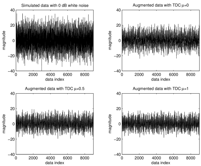
Figure 1: (a) Time series from the Rössler system contaminated with 0 dB additive white noise; (b), (c) and (d) Augmented time series by TDC projectors with $\mu=0,0.5$ and $1$ separately.

Let $\left\{s_{i}\right\}_{i=1}^{M}$ and $\left\{d_{i}\right\}_{i=1}^{M}$ again denote the noisy and clean signals respectively. We consider adding three types of noise contamination to the clean data. The first one is additive white noise $\left\{\xi_{i}\right\}_{i=1}^{M}$ (so that $s_{i}=d_{i}+\xi_{i}$), which follows the normal Gaussian distribution $N(0,1)$. The second one is additive colored noise $\left\{\eta_{i}\right\}_{i=1}^{M}$ (so that $s_{i}=d_{i}+\eta_{i}$), which, as an example, is produced from a third order autoregressive ($AR(3)$) process in the form of $\eta_{i}=0.8\eta_{i-1}-0.5\eta_{i-2}+0.6\eta_{i-3}+\xi_{i}$, where variable $\xi$ follows the normal distribution $N(0,1)$. The last one is multiplicative noise $\left\{\zeta_{i}d_{i}\right\}_{i=1}^{M}$ (so that $s_{i}=(1+\zeta_{i})d_{i}$). As an example, we let $\zeta_{i}=\eta_{i}^{2}$, where $\left\{\eta_{i}\right\}_{i=1}^{M}$ is from the previous $AR(3)$ process, then the noise component $\left\{\zeta_{i}d_{i}\right\}_{i=1}^{M}$ is correlated to the clean data $\left\{d_{i}\right\}_{i=1}^{M}$.

By varying the magnitude of the introduced noise, we have the initial noise level be $20$ dB, $10$ dB, $0$ dB respectively, and for each noise level, we will include $10$ different noise samples from the same process in calculation. We will also study the performance of the projectors under different constraints. As examples, we let TDC $\mu=0$, $0.5$ and $1$ separately. TDC $\mu=0$ will lead to the least-squares (LS) projector based on the SVD technique that appeared in, for example, allen optimal (1, 2, 13). We would need to specify the dimension of the signal-plus-noise subspace so as to group the EOFs and eigenvalues that correspond to the noisy signal and remove the complementary noise subspace, which is essentially related to the problem of choosing the embedding dimension for embedding reconstruction from a scalar time series (see the discussion in johnson generalized (8)). Thus here we adopt the criterion of false nearest neighbor Kennel (9), a method proposed for selection of appropriate embedding dimensions. To apply this criterion in calculation, we utilized the codes implemented in the TISEAN package Tisean (6) and found that the proper dimension size $K$ of the signal-plus-noise subspace is $5$ in our cases. For $\mu=1$, we will obtain the well-know linear minimum mean-squared-error (LMMSE) projector (detailed introductions available in, e.g., trees detection (12)). After all of the calculations, we finally list the performance of these TDC projectors in Table 1. For better comprehension of the presented results, we provide the waveforms of all of the data listed in Table 1 as the supplementary material supplementary (15). To keep our presentation concise, here we only take out the raw data contaminated with $0$ dB additive white noise as an example and depict its waveform of in panel $(a)$ of Fig. (1). For comparison, we also plot the augmented data with TDC$=0,0.5$ and $1$ in panel $(b)$, $(c)$ and $(d)$, whose mean noise levels are $5.88,$ $9.71$ and $10.10$ dB correspondingly.

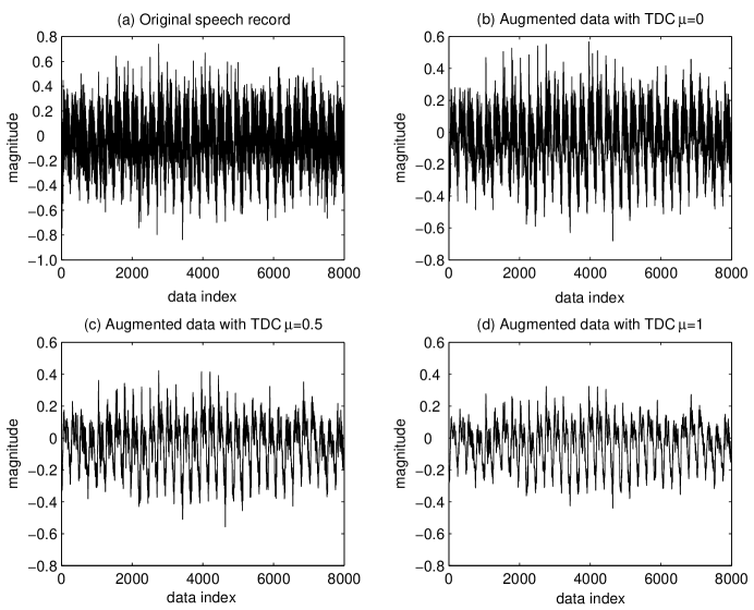
Figure 2: (a) Original speech record; (b), (c) and (d) Speech data output from TDC projectors with $\mu=0,0.5$ and $1$ separately.

From Table 1, we see that for the Rössler system, our algorithm works for all of the three types of contamination. But the data augmentation for additive colored noise is not as obvious as those for additive white noise and multiplicative noise (the possible explanation is explored in the appendix). We also see that, in general, the LMMSE projector has better performance than that of the LS projector in the sense that it can achieve better SNR as defined in Eq. (8).

We then apply our algorithm to a very noisy speech (vowel) data (with $8,000$ data points), which is sampled at $44$ kHz and quantized to $16$ bits. In this case we only know the background noise measured in the period without the signal. It would be preferred if we could produce a set of samples that mimic the behavior of the underlying noise. Here we adopt the pseudo-periodic surrogate (PPS) algorithm small surrogate (11) to generate $9$ surrogates based on the original background noise. With these data sets, the initial SNR of the speech data is estimated to be $-0.32\pm 0.18$ dB via Eq.(8). To introduce phase space projection to the speech data, we let the window size $m=30$ and set the dimension size of signal-plus-noise subspace to be $K=8$, and then apply the TDC projectors $\mathbf{H}$ to its trajectory  matrix. For the LS projector ($\mu=0$), the augmented SNR$=4.36\pm 0.41$ dB. While for TDC $\mu=0.5$ and $1$, the corresponding SNRs increase to $6.28\pm 0.61$ dB and $6.97\pm 0.66$ dB respectively. As an illustration, we plot the waveforms of the original speech record and three projected data under different TDCs in Fig. (2), from which we can see that, the LMMSE projector ($\mu=1$) would lead to a smoother speech waveform (panel (d)) than that of the LS projector (panel (b)). Although the speech data output from the LMMSE projector has lower (signal) magnitudes than those of the speech record from the LS projector, it is still preferred to its rival in speech communication since a smoother data will usually bring better communication quality.

IV Conclusion

In this communication we re-examined the noise reduction technique based on phase space projection. By imposing a constraint on the residual noise, we deduced the optimal time domain constrained projector in the sense of minimizing signal distortion subject to a permissible noise level. We also showed that, in general we need not assume independence between clean signal and noise components as was previously done. This viewpoint was confirmed by our numerical results (see the third column of the calculation results in Table 1).

Appendix

Here let us examine the metric of signal-to-noise ratio (SNR) in more detail. According to the definition in Eq. (8), $SNR=10\log_{10}\left\|d\right\|^{2}/\left\|z-d\right\|^{2},$where $\left\|d\right\|^{2}=\sum\limits_{i=1}^{M}d_{i}^{2}$ and $\left\|z-d\right\|^{2}=$ $\sum\limits_{i=1}^{M}(z_{i}-d_{i})^{2}$. Note that $\left\|d\right\|^{2}=tr(\mathbf{D}^{T}\mathbf{D})/m$ and $\left\|z-d\right\|^{2}=tr(\mathbf{(Z-D)}^{T}\mathbf{(Z-D))/}m$ as $M\rightarrow\infty$, thus

$$SNR=10\log_{10}tr(\mathbf{D}^{T}\mathbf{D})-10\log_{10}tr(\mathbf{(Z-D)}^{T}\mathbf{(Z-D))}.$$

Since $\mathbf{Z=SH}$, we have $tr(\mathbf{(Z-D)}^{T}\mathbf{(Z-D))=}tr(\mathbf{H}^{T}\mathbf{S}^{T}\mathbf{SH})-2tr(\mathbf{D}^{T}\mathbf{SH})+tr(\mathbf{D}^{T}\mathbf{D})$. For the case that the noise and the clean signal are independent. substituting the optimal projector $\mathbf{H}_{\min}$ into the expression, it can be shown that $tr_{\min}(\mathbf{(Z-D)}^{T}\mathbf{(Z-D))=}tr(\mathbf{D}^{T}\mathbf{D})-tr(\mathbf{H}_{\min}\mathbf{D}^{T}\mathbf{D})$. For simplicity, we assume the expectation values $E(d)=E(n)=0$, then $\mathbf{C}_{D}=\mathbf{D}^{T}\mathbf{D/(}M-m+1\mathbf{)}$ and $\mathbf{C}_{N}=\mathbf{N}^{T}\mathbf{N/(}M-m+1\mathbf{)}$ as $M\rightarrow\infty$, where $\mathbf{C}_{D}$ and $\mathbf{C}_{N}$ are the covariance matrix of the clean signal and the noise respectively, and $\mathbf{H}_{\min}$ can be expressed in the form of Eq. (7), or equivalently, $\mathbf{H}_{\min}=\{\mathbf{C}_{D}+\mu^{2}\mathbf{C}_{N}\}^{-1}\mathbf{C}_{D}$. Therefore in this case, we have $tr_{\min}(\mathbf{(Z-D)}^{T}\mathbf{(Z-D))=}tr(\mathbf{C}_{D})-tr(\mathbf{H}_{\min}\mathbf{C}_{D})$, thus the maximal SNR can be expressed by

$$SNR_{\max} = 10\log_{10}tr(\mathbf{C}_{D})-10\log_{10}(tr(\mathbf{C}_{D})$$ (10)

$$-tr(\{\mathbf{C}_{D}+\mu^{2}\mathbf{C}_{N}\}^{-1}\mathbf{C}_{D}^{2})).$$

Through the SVD technique broomhead extracting (2), $\mathbf{C}_{D}$ can be written as $\mathbf{C}_{D}=\mathbf{V}_{D}\mathbf{\Lambda}_{D}\mathbf{V}_{D}^{T}$ , where $\mathbf{V}_{D}$ is the normalized eigenvector matrix of $\mathbf{C}_{D}$, and $\mathbf{\Lambda}_{D}$ is a diagonal matrix whose non-zero elements are the eigenvalues of $\mathbf{C}_{D}$ (in fact $\mathbf{V}_{D}^{T}\mathbf{V}_{D}=\mathbf{I}_{m}$ and $\mathbf{C}_{D}\mathbf{V}_{D}=\mathbf{V}_{D}\mathbf{\Lambda}_{D}$). Similarly, we have $\mathbf{C}_{N}=\mathbf{V}_{N}\mathbf{\Lambda}_{N}\mathbf{V}_{N}^{T}$. Let $\mathbf{V}_{N}=\mathbf{V}_{D}\mathbf{P}_{DN}$ (for better comprehension, $\mathbf{P}_{DN}$ can be thought as a kind of projection from $\mathbf{V}_{N}$ on $\mathbf{V}_{D}$), then $\mathbf{C}_{N}=\mathbf{V}_{D}\mathbf{P}_{DN}\mathbf{\Lambda}_{N}\mathbf{P}_{DN}^{T}\mathbf{V}_{D}^{T}$. Substitute it into Eq. (10), we have

$$SNR_{\max} = 10\log_{10}tr(\mathbf{\Lambda}_{D})-10\log_{10}(tr(\mathbf{\Lambda}_{D})$$

$$-tr(\{\mathbf{\Lambda}_{D}+\mu^{2}\mathbf{P}_{DN}\mathbf{\Lambda}_{N}\mathbf{P}_{DN}^{T}\}^{-1}\mathbf{\Lambda}_{D}^{2})).$$

If the noise components are white, we have $\mathbf{\Lambda}_{N}=\sigma^{2}\mathbf{I}_{m}$ (with $\sigma$ being the standard deviation of the noise process) and $\mathbf{V}_{N}=\mathbf{V}_{D}$ (i.e. $\mathbf{P}_{DN}=\mathbf{I}_{m}$) allen optimal (1). However, for the case of colored noise, usually $\mathbf{P}_{DN}\neq\mathbf{I}_{m}$. Instead it is possible that the absolute value of the elements in $\mathbf{P}_{DN}$ are relatively small. Thus even for the same clean signal $\{d_{i}\}_{i}^{M}$, the $SNR_{\max}$ performance of the colored noise might be much worse than that of the white noise. This fact might explain the observation that the results in Table. I are not that promising for the additive colored noise.

References

- (1) M. R. Allen and L. A. Smith, Phys. Lett. A 234, 419-428 (1997).
- (2) D. S. Broomhead and G. P. King, Physica D 20, 217-236 (1986).
- (3) S. Doclo and M. Moonen, IEEE Trans. Speech Audio Process. 13, 53-69 (2005).
- (4) Y. Ephraim and H. L. V. Trees, IEEE Trans. Speech Audio Process. 3, 251-266 (1995).
- (5) N. Golyandina, V. Nekrutkin and A. Zhigljavsky, Analysis of Time Series Structure: SSA and Related Techniques (Chapman & Hall/CRC, 2001).
- (6) R. Hegger, H. Kantz, and T. Schreiber, Chaos 9, 413-435 (1999).
- (7) Y. Hu, and P. C. Loizou, IEEE Trans. Speech Audio Process. 11, 334-341 (2003).
- (8) M. T. Johnson and R. J. Povinelli, Physica D 201, 306-317 (2005).
- (9) M. B. Kennel, R. Brown, and H. D. I. Abarbanel, Phys. Rev. A 45, 3403-3411 (1992).
- (10) H. Lütkepohl, Introduction to Multiple Time Series Analysis (Springer-Verlag, Berlin, 1991).
- (11) M. Small, D. Yu, and R.G. Harrison, Phys. Rev. Lett. 87, 188101 (2001).
- (12) H. L. V. Trees, Detection, Estimation, and Modulation Theory, Vol. I (Wiley, New York, 1968).
- (13) R. Vautard and M. Ghil, Physica D 35, 395-424 (1989).
- (14) We share the viewpoint with Golyandina et al that (currently) there is no universal rule for the optimization problem of . For general suggestions on choosing , readers are referred to (golyandina analysis, 5, p.53). In practice it is also possible that is a constant, for instance, the signal length in a frame of speech record.
- (15) See EPAPS Document No. [please insert the document number in publication] for the waveforms of all of the data listed in Table 1. This document can be reached via a direct link in the online article’s HTML reference section or via the EPAPS homepage (http://www.aip.org/pubservs/epaps.html).