Mapping Model of Chaotic Phase Synchronization

Abstract

A coupled map model for the chaotic phase synchronization and its desynchronization phenomenon is proposed. The model is constructed by integrating the coupled kicked oscillator system, kicking strength depending on the complex state variables. It is shown that the proposed model clearly exhibits the chaotic phase synchronization phenomenon. Furthermore, we numerically prove that in the region where the phase synchronization is weakly broken, the anomalous scaling of the phase difference rotation number is observed. This proves that the present model belongs to the same universality class found by Pikovsky et al.. Furthermore, the phase diffusion coefficient in the de-synchronization state is analyzed.

1 Introduction

Coupled chaos systems are not only theoretically interesting but also important from the viewpoint of the application to engineering and biology [1, 2, 3]. Dynamical behaviors observed in coupled oscillator systems depend on the number of chaotic oscillators as well as the coupling form. As the number of oscillators is increased, the variety and the complexity of dynamical behaviors increase. One of the eminent characteristics of the coupled chaos systems is the synchronization and its breakdown. For a coupled system consisted of identical chaotic oscillators, it was shown that the oscillators can completely synchronize under certain conditions [4]. This phenomenon is called either the chaotic complete synchronization or the chaotic Huygens phenomenon [4]. On the other hand, even when two oscillators have a mismatch in characteristic, they can show the so called chaotic phase synchronization for a certain region of coupling strength [5].

It is well known that the coupled map system played a significant role in the study of complete synchronization [7, 8]. Particularly, coupled one-dimensional map system is a typical model in discussing the chaos synchronization-desynchronization phenomenon. In contrast to the complete synchronization, coupled mapping model for chaotic phase synchronization-desynchronization phenomenon is not studied so much because of the lack of suitable mapping model for coupled phase synchronization. The aims of the present paper are to propose a coupled mapping model for chaotic phase synchronization and then to examine the universality of the breakdown of synchronization so far mainly studied for the coupled Rössler system.

The present paper is constructed as follows. In Sec. 2, we propose a general, linearly coupled mapping system for coupled chaotic oscillators which show either periodic or chaotic characteristics. The model is constructed by integrating the equations of motion for oscillator variables with a state dependent kicking term. In Sec. 3, using a two oscillators system, we discuss general characteristics of the system, and then study the phase difference statistics associated with the breakdown of the chaotic phase synchronization. We give summary and concluding remarks in Sec. 4.

2 Mapping model of coupled oscillatory chaotic systems

First, consider the linear equations of motion

$$\dot{\psi}(t) = p,$$ (1)

$$\tau\dot{p}(t) = i\omega\psi-p,$$ (2)

where $\psi$ and $p$ are complex variables, $\tau$ is a positive number and $\omega$ is a real number. In the limit $\tau\rightarrow 0$, the above equations reduce to $\dot{\psi}=i\omega\psi$, the equation of motion for a harmonic oscillator. So, $\omega$ has the meaning of the eigenfrequency of the oscillator, and the above set of equations of motion turns out to describe a harmonic oscillator slightly modulated by the introduction of the “inertia term” $\tau\dot{p}$. The above equations of motion can be solved as $\psi(t)\sim e^{\lambda t},\ p(t)\sim e^{\lambda t}$, with the characteristic exponents $\lambda=\tau^{-1}(-1\pm\sqrt{1+4i\tau\omega})/2$. For small $\tau$, they are written as $\lambda=i\omega+\tau\omega^{2},\ -\tau^{-1}-i\omega.$ One should note that in the presence of the inertia term, the above harmonic oscillation is unstable.

We consider the periodically-kicked harmonic oscillator system

$$\dot{\psi}(t) = p,$$ (3)

$$\tau\dot{p}(t) = i\omega\psi-p+F_{a}(\psi,\psi^{*})\cdot\sum_{n=-\infty}^{+\infty}\delta(t-t_{n}),$$ (4)

$(t_{n}=nT)$, where $T$ is the period of kicking and is taken to be unity without loss of generality. $F_{a}(\psi,\psi^{*})$ is the state-dependent complex amplitude of kicking, $a$ standing for a set of parameters which characterizes the oscillator. Let us solve the above equation for $t_{n}-\delta\leq t\leq t_{n+1}-\delta$, $\delta$ being a positive infinitesimal quantity. Then, taking the limit $\tau\rightarrow 0$, one finds that the above set of equations of motion reduces to

$$\psi_{n+1}=e^{i\omega}f_{a}(\psi_{n},\psi_{n}^{*})$$ (5)

and $p(t_{n+1}-\delta)=i\omega\psi_{n+1}$, where we noticed that $\psi_{n}\equiv\psi(t_{n}-\delta)=\psi(t_{n})$ because of the continuity of $\psi(t)$ at $t_{n}$. Here we defined

$$f_{a}(\psi,\psi^{*})=\psi+F_{a}(\psi,\psi^{*}).$$ (6)

Equation ($2\cdot 5$) with eq. ($2\cdot 6$) is the mapping system for the kicked-oscillator system ($2\cdot 3$) and ($2\cdot 4$). One should note that the mapping model ($2\cdot 5$) has two types of characteristic parameters. One is the eigenfrequency $\omega$ of the oscillation and therefore is relevant to the phase degree of freedom, and the other is the parameter set $a$, which is regarded as the control parameter mainly relevant to the amplitude dynamics of oscillation.

In the above, we proposed a mapping model relevant to a chaotic dynamics showing a well-defined oscillation. Next, we will construct a mapping system consisted of coupled oscillators. As an example, consider the two oscillators system coupled to each other,

$$\dot{\psi}^{(j)} = p^{(j)},$$ (7)

$$\tau\dot{p}^{(j)} = i\omega_{j}\psi^{(j)}-p^{(j)}+F_{a_{j}}(\psi^{(j)},\psi^{(j)*})\cdot\sum_{n=-\infty}^{+\infty}\delta(t-t_{n})+\frac{K}{2}(\psi^{(k)}-\psi^{(j)})$$ (8)

for $(j,k)=(1,2),\ (2,1)$. The last term of eq. ($2\cdot 8$) represents the coupling and $K$ is the coupling constant. In the present paper, unless it is stated, $K$ is kept to be non-negative. For the coupled $N$-elements system, the equations of motion for the $j$-th oscillator are written as

$$\dot{\psi}^{(j)} = p^{(j)},$$ (9)

$$\tau\dot{p}^{(j)} = i\omega_{j}\psi^{(j)}-p^{(j)}+F_{a_{j}}(\psi^{(j)},\psi^{(j)*})\cdot\sum_{n=-\infty}^{+\infty}\delta(t-t_{n})+{\cal D}\psi^{(j)}.$$ (10)

Here ${\cal D}\psi^{(j)}$ represents the linear coupling term. Particularly, for the $N=2$ model given in eqs. ($2\cdot 7$) and ($2\cdot 8$), we get ${\cal D}\psi^{(1,2)}=(K/2)(\psi^{(2,1)}-\psi^{(1,2)}).$

Solving the above equations of motion for $t_{n}-\delta\leq t\leq t_{n+1}-\delta$ and taking the limit $\tau\rightarrow 0$, one obtains the coupled map system

$$\psi_{n+1}^{(j)} = e^{i\omega_{j}+{\cal D}}f_{a_{j}}(\psi_{n}^{(j)},\psi_{n}^{(j)*})$$ (11)

$$= \sum_{k}J_{jk}e^{i\omega_{k}}f_{a_{k}}(\psi_{n}^{(k)},\psi_{n}^{(k)*}),$$

for $\psi_{n}^{(j)}\equiv\psi^{(j)}(t_{n}-\delta)=\psi^{(j)}(t_{n})$ and $p^{(j)}(t_{n+1}-\delta)=(i\omega_{j}+{\cal D})\psi_{n+1}^{(j)}$, where $f_{a}(\psi,\psi^{*})$ is the same as in eq. ($2\cdot 6$). The coupling constant $J_{jk}$ has been defined as follows. Let us introduce the matrix $\hat{\Lambda}$ with the $jk$ element $\Lambda_{jk}$ defined by

$$(i\omega_{j}+{\cal D})g_{j}=\sum_{k}\Lambda_{jk}g_{k}$$ (12)

for an arbitrary quantity $g_{j}$ defined for the oscillator $j$. The interaction kernel $J_{jk}$ in eq. ($2\cdot 11$) is defined via

$$e^{i\omega_{j}+{\cal D}}g_{j}=\sum_{k}\left(e^{\hat{\Lambda}}\right)_{jk}g_{k}=\sum_{k}J_{jk}e^{i\omega_{k}}g_{k}.$$ (13)

Equation ($2\cdot 11$) together with eqs. ($2\cdot 12$) and ($2\cdot 13$) is the fundamental result of the present paper.

Particularly, if the coupling term has the form

$${\cal D}g_{j}=\sum_{k=1}^{N}K_{jk}(g_{k}-g_{j}),$$ (14)

where $K_{jk}$ is the coupling constant, then the matrix element is given by

$$\Lambda_{jk}=i\omega_{j}\delta_{jk}+K_{jk}-\left(\sum_{\ell=1}^{N}K_{j\ell}\right)\delta_{jk}.$$ (15)

If all characteristic frequencies are same, i.e., $\omega_{1}=\omega_{2}=\cdots=\omega_{N}\equiv\omega$, and the coupling operator satisfies the condition $\sum_{j}{\cal D}g_{j}=0$ and therefore $\sum_{j}J_{jk}=1$, then eq. ($2\cdot 11$) is rewritten as

$$\psi_{n+1}^{(j)}=e^{i\omega}\left\{f_{a_{j}}(\psi_{n}^{(j)},\psi_{n}^{(j)*})+\sum_{k}J_{jk}\left[f_{a_{k}}(\psi_{n}^{(k)},\psi_{n}^{(k)*})-f_{a_{j}}(\psi_{n}^{(j)},\psi_{n}^{(j)*})\right]\right\}.$$ (16)

Furthermore, for the global coupling ${\cal D}g_{j}=(K/N)\sum_{k=1}^{N}(g_{k}-g_{j}),$ one obtains $J_{jk}=K/N$ for any combinations of $j$ and $k$. In addition, when the system characteristics are all the same ($a_{1}=a_{2}=\cdots=a_{N}\equiv a$), one finds that the equations of motion under consideration has the complete synchronization $\psi_{n}^{(1)}=\psi_{n}^{(2)}=\cdots=\psi_{n}^{(N)}\equiv\psi_{n}^{0}$, which obeys $\psi_{n+1}^{0}=e^{i\omega}f_{a}(\psi_{n}^{0},\psi_{n}^{0*})$ irrespectively of the coupling strength. This fact suggests the possibility of the existence of the transition between the complete synchronization and its broken state. Details will be given in Sec. 3 for the two-oscillators system.

3 Chaotic phase synchronization in a two oscillators system

In this section, we study the synchronization and desynchronization for the coupled maps model of a two oscillators system proposed in the preceding section. For the coupling term ${\cal D}g_{1,2}=(K/2)(g_{2,1}-g_{1,2})$, we get

$$\hat{\Lambda}=\left(\begin{array}[]{cc}i\omega_{1}-\frac{K}{2}&\frac{K}{2}\\ \frac{K}{2}&i\omega_{2}-\frac{K}{2}\end{array}\right).$$ (19)

This immediately gives the coupled map system

$$\psi_{n+1}^{(1)}=J_{K}(\omega_{1}-\omega_{2})e^{i\omega_{1}}f_{a_{1}}(\psi_{n}^{(1)},\psi_{n}^{(1)*})+J_{K}^{\prime}(\omega_{1}-\omega_{2})e^{i\omega_{2}}f_{a_{2}}(\psi_{n}^{(2)},\psi_{n}^{(2)*}),$$ (20)

$$\psi_{n+1}^{(2)}=J_{K}^{\prime}(\omega_{2}-\omega_{1})e^{i\omega_{1}}f_{a_{1}}(\psi_{n}^{(1)},\psi_{n}^{(1)*})+J_{K}(\omega_{2}-\omega_{1})e^{i\omega_{2}}f_{a_{2}}(\psi_{n}^{(2)},\psi_{n}^{(2)*}),$$ (21)

where the coupling constants are

$$J_{K}(\Delta\omega) = e^{-\frac{i}{2}\Delta\omega}e^{-\frac{K}{2}}\left[\cosh\frac{\sqrt{K^{2}-(\Delta\omega)^{2}}}{2}+i\Delta\omega\frac{\sinh\frac{\sqrt{K^{2}-(\Delta\omega)^{2}}}{2}}{\sqrt{K^{2}-(\Delta\omega)^{2}}}\right],$$ (22)

$$J_{K}^{\prime}(\Delta\omega) = e^{\frac{i}{2}\Delta\omega}e^{-\frac{K}{2}}\frac{K\sinh\frac{\sqrt{K^{2}-(\Delta\omega)^{2}}}{2}}{\sqrt{K^{2}-(\Delta\omega)^{2}}}.$$ (23)

It should be noted that the coupling constants satisfy $J_{K}(\Delta\omega)^{*}=J_{K}(-\Delta\omega)$ and $J_{K}^{\prime}(\Delta\omega)^{*}=J_{K}^{\prime}(-\Delta\omega)$.

3.1 General characteristics of the two oscillators system

Since $J_{0}(\Delta\omega)=1$ and $J_{0}^{\prime}(\Delta\omega)=0$, oscillators are independent of each other for $K=0$. On the other hand, for $K\rightarrow\infty$, noting $J_{\infty}(\Delta\omega)=\frac{1}{2}e^{-\frac{i}{2}\Delta\omega}=J_{\infty}^{\prime}(\Delta\omega)^{*}$, we obtain

$$\psi_{n}^{(1)} = \psi_{n}^{(2)}\equiv\psi_{n}^{0},$$ (24)

$$\psi_{n+1}^{0} = \frac{1}{2}e^{\frac{i}{2}(\omega_{1}+\omega_{2})}\left[f_{a_{1}}(\psi_{n}^{0},\psi_{n}^{0*})+f_{a_{2}}(\psi_{n}^{0},\psi_{n}^{0*})\right].$$ (25)

This result implies that even if the characteristics of two oscillators are different, the system shows a complete synchronization in the strong coupling limit $K\rightarrow\infty$. It should be noted that for the coupled system consisted of identical oscillators the complete synchronization is achieved irrespectively of the strength as a particular motion, while the present synchronization for non-identical oscillators is observed only when the $K\rightarrow\infty$ limit. On the other hand, if the system parameters $\omega_{j}$ and $a_{j}$ are different from each other, the system does not show a complete synchronization. Nevertheless, we expect that there exists a certain kind of synchronization state if the coupling constant $K$ is suitably chosen, which is nothing but the phase synchronization [5]. This will be studied in the following subsection.

Particularly, if $\omega_{1}=\omega_{2}\equiv\omega$ and $a_{1}=a_{2}\equiv a$, i. e. , the two oscillators are identical, then the coupled map system is written as

$$\psi_{n+1}^{(1)} = e^{i\omega}\left\{f_{a}(\psi_{n}^{(1)},\psi_{n}^{(1)*})+J_{k}^{\prime}\left[f_{a}(\psi_{n}^{(2)},\psi_{n}^{(2)*})-f_{a}(\psi_{n}^{(1)},\psi_{n}^{(1)*})\right]\right\},$$ (26)

$$\psi_{n+1}^{(2)} = e^{i\omega}\left\{f_{a}(\psi_{n}^{(2)},\psi_{n}^{(2)*})+J_{k}^{\prime}\left[f_{a}(\psi_{n}^{(1)},\psi_{n}^{(1)*})-f_{a}(\psi_{n}^{(2)},\psi_{n}^{(2)*})\right]\right\},$$ (27)

where $J_{K}^{\prime}=(1-e^{-K})/2$. In this case, the particular, complete synchronization state exists and the dynamical variable $\psi_{n}^{0}(=\psi_{n}^{(1)}=\psi_{n}^{(2)})$ obeys $\psi_{n+1}^{0}=e^{i\omega}f_{a}(\psi_{n}^{0},\psi_{n}^{0*})$. Around the complete synchronization state, the small deviations $\delta\psi_{n}^{(1)}=\psi_{n}^{(1)}-\psi_{n}^{0}$ and $\delta\psi_{n}^{(2)}=\psi_{n}^{(2)}-\psi_{n}^{0}$ from the complete synchronization obey

$$\delta\psi_{n+1}^{+} = e^{i\omega}(G_{1,n}\delta\psi_{n}^{+}+G_{2,n}\delta\psi_{n}^{+*}),$$ (28)

$$\delta\psi_{n+1}^{-} = e^{i\omega}e^{-K}(G_{1,n}\delta\psi_{n}^{-}+G_{2,n}\delta\psi_{n}^{-*}),$$ (29)

where $\delta\psi_{n}^{\pm}=(\delta\psi_{n}^{(1)}\pm\delta\psi_{n}^{(2)})/2$, and $G_{1,n}=\partial f_{a}(\psi_{n}^{0},\psi_{n}^{0*})/\partial\psi_{n}^{0}$ and $G_{2,n}=\partial f_{a}(\psi_{n}^{0},\psi_{n}^{0*})/\partial\psi_{n}^{0*}$. It should be noted that the two equations of motion for $\delta\psi_{n}^{\pm}$ are separated from each other, and the first equation is identical to the perturbation equation $\delta\psi_{n+1}^{0}=e^{i\omega}(G_{1,n}\delta\psi_{n}^{0}+G_{2,n}\delta\psi_{n}^{0*})$ for the small change of the initial condition of the element dynamics. Let $\lambda$ be the largest Lyapunov exponent of the element dynamics. One finds that

$$|\delta\psi_{n}^{+}|\sim e^{\lambda n}|\delta\psi_{0}^{+}|$$ (30)

for large $n$. The exponent $\lambda$ shows the characteristic of the uncoupled system and is free from the stability of the complete synchronization. On the other hand, the second equation gives

$$|\delta\psi_{n}^{-}|=\frac{1}{2}|\psi_{n}^{(2)}-\psi_{n}^{(1)}|\sim e^{\lambda_{\perp}n}|\delta\psi_{0}^{-}|,$$ (31)

where

$$\lambda_{\perp}=\lambda-K.$$ (32)

The parameter $\lambda_{\perp}$ called the transverse Lyapunov exponent or the stability parameter determines the stability of the complete synchronization [4]. Namely, if $\lambda_{\perp}<0$, the complete synchronization is linearly stable. On the other hand, if $\lambda_{\perp}>0$, the complete synchronization is unstable. If the element dynamics is periodic, then $\lambda<0$ and therefore $\lambda_{\perp}<0$, which implies that the complete synchronization is linearly stable. On the other hand, for a chaotic element dynamics ($\lambda>0$), the system shows the transition at $K=\lambda(\equiv K_{c})$ as the coupling strength $K$ is decreased from above $K_{c}$, and one observes the on-off (modulated) intermittency for $K$ slightly below $K_{c}$ [9, 10].

3.2 Chaotic phase synchronization and its breakdown

In the present paper, as a model of element dynamics, we use the mapping function

$$f_{a}(\psi,\psi^{*})=[a-(1+ib)|\psi|^{2}]\psi,$$ (33)

where the parameters $a$ and $b$ are chosen in such a way that the dynamics $\psi_{n+1}^{(j)}=e^{i\omega_{j}}f_{a_{j}}(\psi_{n}^{(j)},\psi_{n}^{(j)*})$ shows a chaotic behavior. One should note that the statistical characteristic of the isolated element dynamics is free from the choice of $\omega_{j}$ because the local dynamics does not depend on the eigenfrequency after the replacement $\psi_{n}^{(j)}\rightarrow e^{i\omega_{j}n}\psi_{n}^{(j)}$. A trajectory of the element dynamics ($3\cdot 15$) for $\omega=0.08,a=2.55$ and $b=0$ is shown in Fig. 1. Figure 2 depicts how the trajectories depend on $b$. One observes that depending on $b$, the isolated dynamics shows various characteristics. In later numerical experiments of coupled map system, we use the same values for $a$ and $b$ as $a_{1}=a_{2}=2.55$ and $b_{1}=b_{2}=0$ for which the element dynamics are chaotic, where the largest Lyapunov exponent $\lambda$ is about 0.144, and the frequency parameters $\omega_{1}$ and $\omega_{2}$ are chosen to be set as $\Delta\omega=\omega_{1}-\omega_{2}=0.08$ except the figure 4. One should note that in the present model only the difference of eigenfrequencies is relevant. It was numerically proved that as far as $b$ is small enough, the introduction of non-vanishing $b_{j}$ does not change the qualitative results found for $b_{j}=0$.

Figure 1: Trajectory for the element dynamics ($2\cdot 5$) with the mapping function ($3\cdot 15$), where $\omega=0.03,a=2.55$ and $b=0$. The dynamics is chaotic with the largest Lyapunov exponent $\lambda=0.144$.

Let $\theta_{n}^{(j)}$ be the phase of $\psi_{n}^{(j)}$, i.e., $\psi_{n}^{(j)}=|\psi_{n}^{(j)}|e^{i\theta_{n}^{(j)}}$. It should be noted that as far as the phase variation is small enough, the phase dynamics of $\theta_{n}^{(j)}$ is uniquely determined even for a coupled system. For the control parameters $a_{j}$ and $b_{j}$ used in the present paper, the phase variations are small enough. The phase difference $\Delta\theta_{n}=\theta_{n}^{(1)}-\theta_{n}^{(2)}$ obeys the equation of motion

$$\Delta\theta_{n+1}=\Delta\theta_{n}+\alpha_{n}(\Delta\theta_{n}),$$ (34)

where $\alpha_{n}(\Delta\theta)$, which is uniquely determined by eqs. ($3\cdot 2$) and ($3\cdot 3$), is a $2\pi$-periodic function of $\Delta\theta$, i.e., $(\alpha_{n}(\Delta\theta+2\pi)=\alpha_{n}(\Delta\theta))$. The integration of the above equation yields

$$\Delta\theta_{n}=\Delta\theta_{0}+\sum_{m=0}^{n-1}\alpha_{m}(\Delta\theta_{m}).$$ (35)

By taking the statistical average of the above equation, which is equivalent to the time average with the ergodicity assumption, the angular velocity of the phase difference (rotation number) is given by

$$\Delta\Omega=\lim_{n\rightarrow\infty}\frac{1}{n}\sum_{m=0}^{n-1}\alpha_{m}(\Delta\theta_{m})=\langle\alpha\rangle,$$ (36)

where $\langle\cdots\rangle$ is the statistical average over an ensemble representing the steady state of the present chaos. Therefore, the average value of the phase difference obeys

$$\langle\Delta\theta_{n}\rangle=\Delta\theta_{0}+\Delta\Omega\cdot n.$$ (37)

  

  

  

Figure 2: Trajectories for the element dynamics ($2\cdot 5$) with the mapping function ($3\cdot 15$) for $a=2.55$ and various values of $b$. The abscissa and the ordinate are respectively ${\rm Re}(e^{-i\omega}\psi_{n})$ and ${\rm Im}(e^{-i\omega}\psi_{n})$. Trajectories do not depend on the value of $\omega$ for the mapping ($3\cdot 15$).

Figure 3 shows temporal evolutions of the phase difference for different values of the coupling strength $K$. One observes that depending on $K$, the coupled mapping system exhibits chaotic phase synchronization ($\Delta\Omega=0$). Figure 4 displays how the rotation number $\Delta\Omega$ depends on $K$ and $\Delta\omega(=\omega_{1}-\omega_{2})$. One finds that under the change of either $K$ or $\Delta\omega$ a clear transition between phase synchronization and phase desynchronization state occurs.

Figure 3: Temporal evolution of phase differences for the coupled two maps system. For $K=0.081$, the phase synchronization is achieved.

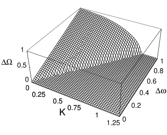
Figure 4: The rotation number $\Delta\Omega$ depends on both the eigenfrequency mismatch $\Delta\omega(=\omega_{1}-\omega_{2})$ and the coupling constant $K$. For $\Delta\Omega=0$, the phase synchronization is achieved.

In order to study the critical behavior of $\Delta\Omega$ as the coupling strength $K$ is decreased by keeping $\Delta\omega$ constant to be 0.08, the quantity $(\Delta\Omega)^{2}$ is plotted as a function of $K$ in Fig. 5(a). The figure suggests that the critical behavior

$$\Delta\Omega\sim(K_{*}-K)^{\frac{1}{2}}$$ (38)

holds in the region $K<K_{*}$, where $K_{*}(\approx 0.0612)$ is a characteristic value of $K$ being below $K_{c}(\approx 0.0804)$, the desynchronization point, i.e., $\Delta\Omega=0$ for $K>K_{c}$. The critical behavior $(3\cdot 20)$ is identical to that of the saddle-node bifurcation, and is well-known in association with the existence of the type I intermittency. Figure 5(b) shows the numerical result for the $K$ region below the onset point $K_{c}$ of the chaotic phase synchronization. Slightly below $K_{c}$, the rotation number turns out to take the asymptotic form

$$\Delta\Omega\sim\exp\left[-c\cdot(K_{c}-K)^{-\frac{1}{2}}\right],$$ (39)

instead of the saddle-node type, where $c$ is a positive constant. This behavior is a result of chaotic, one may say, “stochastic” emergence of the saddle-node type channel, and has been reported near the desynchronization point in a phenomenological mapping model [13] and experimentally in the modulated CO₂ laser system [12]. So, the present model belongs to the same universality class of chaotic phase synchronization showing the above two different critical behaviors.

 

Figure 5: Critical behaviors of the rotation number $\Delta\Omega$ as functions of the coupling constant $K$.

The fluctuation of the phase difference $\Delta\theta_{n}$ from the average value ($3\cdot 19$) is evaluated with the variance

$$\sigma_{n}^{2}\equiv\langle(\Delta\theta_{n}-\langle\Delta\theta_{n}\rangle)^{2}\rangle.$$ (40)

It is expected that by assuming the mixing property of $\alpha_{n}(\Delta\theta_{n})$, the variance obeys the diffusion law

$$\sigma_{n}^{2}=2Dn$$ (41)

for large $n$, where the diffusion coefficient is given by $D=(1/2)\sum_{n=-\infty}^{\infty}C_{|n|}$ with $C_{n}=\langle\delta\alpha_{n}(\Delta\theta_{n})\delta\alpha_{0}(\Delta\theta_{0})\rangle,\ (\delta\alpha_{n}=\alpha_{n}-\langle\alpha\rangle)$. In the present paper, the diffusion coefficients were calculated with the asymptotic form (3.23) for various values of $K$ by keeping $\Delta\omega=0.08$. Results are shown in Fig. 6. One observes an anomalous enhancement of the diffusion coefficient near $K_{*}$, the lower synchronization-desynchronization transition point. Figure 7 displays the relation between the rotation number and the diffusion coefficient. One observes a linear relation $D\sim\Delta\Omega$ for $K$ slightly below $K_{c}$. This fact agrees with the observation in the coupled Rössler system [14]. The numerical result shows $D/\Delta\Omega\approx 2.7$.

Figure 6: The rotation number $\Delta\Omega$ and the phase diffusion coefficient $D$ below the breakdown point $K_{c}$ of chaotic phase synchronization. The diffusion coefficient shows an enhancement slightly below the breakdown point of the phase synchronization.

Figure 7: The relation between the phase diffusion coefficient and the rotation number near the breakdown point of the chaotic phase synchronization. One observes a linear relation $D\sim\Delta\Omega$.

4 Summary and concluding remarks

In the present paper, we proposed a mapping model of coupled chaotic oscillator system composed of element dynamics each of which has a periodic oscillation characteristic in an uncoupled case. An oscillation has two degrees of freedom, phase and amplitude. Parameters contained in dynamical systems described by differential equations of motion for describing oscillatory behaviors generically control both the phase and the amplitude simultaneously. On the other hand, the present mapping model, the parameter $\omega$ mainly controls the phase dynamics and the parameter $a$ the amplitude dynamics. Therefore, in order to study the characteristic dynamics of the phase and the amplitude separately, the present mapping model of oscillatory dynamics is considered to be more convenient to analyze chaotic phase synchronization than the differential equation system such as the Rössler model.

By making use of concrete coupled two maps system, it was shown that the present coupled map system shows the phase synchronization-desynchronization phenomenon. We found that when the amplitude synchronization is achieved, after the breakdown of the phase synchronization the rotation number turns out to show a normal scaling ($3\cdot 20$). However, since this characteristic is quite particular to the element map used in the present paper, in general no amplitude synchronization is expected to be observed, and it may be concluded that sufficiently near the transition point the anomalous scaling ($3\cdot 21$) is ubiquitously observed. In this sense the present two maps system belongs to the universality class of that reported in Ref. 13). Furthermore, we studied the phase diffusion coefficient, and observed that its critical behaviors are the same as those found in Ref. 14).

So far, mapping models of coupled chaos systems, particularly coupled one-dimensional mapping models, have been extensively studied to clarify their varieties of dynamical phenomena as well as mathematical structures of their dynamical behaviors. The proposed coupled map model composed of chaotic oscillator elements which show well-defined limit-cycle type oscillation characteristics is expected to contribute to the progress in the study of the phase synchronization-desynchronization phenomenon in a wide class of coupled chaos systems.

References

• [1] A. Pikovsky, M. Rosenblum and J. Kurths, Synchronization, (Cambridge Univ. Press, Cambridge, 2001).
• [2] E. Mosekilde, Yu. Maistrenko and D. Postnov, Chaotic Synchronization, Applications to living systems, (World Scientific, Singapore, 2002).
• [3] V. S. Anishchenko, V. V. Astakhov, A. B. Neiman et al., Nonlinear Dynamics of Chaotic and Stochastic Systems, (Springer, Berlin, 2002).
• [4] H. Fujisaka and T. Yamada, Prog. Theor. Phys. 69, 32 (1983).
• [5] M. G. Rosenblum, A. S. Pikovsky and J. Kurths, Phys. Rev. Lett. 76, 1804 (1996).
• [6] S. Boccaletti, J. Kurths, G. Osipov, D.L. Valladares, and C.S. Zhou, Phys. Rep. 366, 1 (2002).
• [7] T. Yamada and H. Fujisaka, Prog. Theor. Phys. 70, 1240 (1983).
• [8] K. Kaneko, Physica D41, 137 (1990).
• [9] H. Fujisaka and T. Yamada, Prog. Theor. Phys. 74, 918 (1985).
• [10] H. Fujisaka and T. Yamada, Prog. Theor. Phys. 75, 1087 (1986).
• [11] T. Yamada and H. Fujisaka, Prog. Theor. Phys. 76, 582 (1986).
• [12] S. Boccaletti, E. Allaria, R. Meucci and F. T. Arecchi, Phys. Rev. Lett.  89, 194101 (2002).
• [13] A. Pikovsky, G. Osipov, M. Rosenblum, M. Zaks and J. Kurths, Phys. Rev. Lett. 79, 47 (1997).
• [14] H. Fujisaka, T. Yamada, G. Kinoshita and T. Kono, Physica D, in press.
• [15] N. F. Rulkov, M. M. Sushchik, L. S. Tsimring, H. D. I. Abarbanel, Phys. Rev. E 51, 980 (1995).
L. Kocarev and U. Parlitz, Phys. Rev. Lett. 76, 1816 (1996).
• [16] M. G. Rosenblum, A. S. Pikovsky and J. Kurths, Phys. Rev. Lett. 78, 4193 (1997).