Uniform approximation of barrier penetration in phase space

Abstract

A method to approximate transmission probabilities for a nonseparable multidimensional barrier is applied to a waveguide model. The method uses complex barrier-crossing orbits to represent reaction probabilities in phase space and is uniform in the sense that it applies at and above a threshold energy at which classical reaction switches on. Above this threshold the geometry of the classically reacting region of phase space is clearly reflected in the quantum representation. Two versions of the approximation are applied. A harmonic version which uses dynamics linearised around an instanton orbit is valid only near threshold but is easy to use. A more accurate and more widely applicable version using nonlinear dynamics is also described.

I Introduction

Semiclassical approaches to multidimensional tunnelling lead to very interesting problems in complexified classical dynamics, often with incompletely understood solutions. For example, recent work in references Shudo ; aY00 ; Takahashi ; TYK ; Onishi ; Julia has shown that nontrivial geometrical structure such as complex homoclinic intersections have an important role to play in multidimensional barrier penetration and that even complex chaos can be relevant. Given the difficulty inherent in a systematic treatment of multidimensional tunnelling as a result of such issues, it is perhaps surprising that a relatively simple description can be given of barrier penetration at a critical energy where classically allowed transmission mechanisms turn on and where primitive semiclassical approximations must be replaced by somewhat more complicated uniform ones.

An approach which achieves this has been proposed in references sC04 and sc05 and in this paper we apply the method explicitly to a model waveguide problem. The model is chosen to be rather simple so that fully quantum calculations are easy to perform accurately for purposes of comparison. We emphasise, however, that semiclassical aspects of the calculation are as easily applied to other problems, provided the topology is similar, and provide a description, for example, of collinear atom-diatom reactions. For that reason we use the terminology of chemical reactions in this paper and equate the probability of transmission with a probability of reaction. In fact the approach we describe here provides a natural means of visualising the quantum scattering problem in phase space and as such shows an interesting connection with classical transition state theories of chemical reaction. These classical theories have recently been of interest because the periodic-orbit dividing surface (PODS) construction Pechukas ; PODS2 has been generalised to arbitrary dimensions using the construction of normally hyperbolic invariant manifolds (NHIMS) Jaffe ; Uzer ; WW ; HCN ; LW . The classical constructions emerge naturally in our semiclassical approximation and we note that even though the illustrations offered here are in two degrees of freedom there are straightforward generalisations to higher dimensional problems where the full generality of the NHIM construction comes into play.

The approximation we use can be stated very simply as an abstract operator equation but for explicit illustration we present results in phase space, using the Wigner-Weyl calculus. In particular, we define a Weyl symbol of a transmission matrix which represents, in an averaged sense, a reaction probability as a function of phase space. We find that above threshold the support of this Weyl symbol closely mimics the shape of the classically reacting region but the Weyl symbol itself also incorporates tunnelling and other quantum effects. Notation and details for this construction are set out in section II.

We implement two versions of the theory. First, a harmonic approximation derived in sC04 is applied in section III whose classical input consists simply of an instanton orbit, along with its action and monodromy matrix. This approximation works when the classically reacting region is a small neighbourhood of the initial condition for the instanton orbit and is harmonic in the sense that it uses linearised dynamics generated by an elliptic quadratic Hamiltonian on the Poincaré section. This harmonic version covers the threshold case where classical reaction switches on as a function of energy and is relatively easy to apply. It fails however when the energy is too far above threshold and the classically reacting region is too large to be adequately described by linearised dynamics.

A semiclassical approximation that is more accurate and has greater range has been derived in sc05 and this is applied in section IV. This version uses fully nonlinear dynamics to extend further from the instanton orbit. Like the harmonic version it can be stated quite simply as an abstract operator equation but its practical implementation is more difficult. Difficulty arises primarily because we must invert an operator constructed semiclassically as an evolution operator and this inversion cannot at present be achieved in closed form. In this paper we achieve that inversion using numerical methods and while this aspect of the approach needs further work to provide an appealing semiclassical method, we can verify unambiguously that the nonlinear version of the theory is capable of describing the quantum transmission problem very accurately (see Figure 8).

We conclude this section by outlining how these results relate to existing work. The basic formalism here of relating scattering to complex barrier-crossing orbits goes back to the work of Miller and coworkers MG ; MillerSmatrix on the classical $S$-matrix. Our intent is to describe a simple uniform extension of this approach which applies at the boundary of classical reaction where the fate of classical orbits changes discontinuously. What allows us to make progress is that we do not directly describe the $S$-matrix but instead consider a transmission matrix derived from it which gives probabilities rather than amplitides. The advantage of this problem is that contributing orbits at the boundary of classical reaction depend smoothly on initial conditions, despite the singular nature of real orbits there sC04 , and give simple semiclassical expressions. This uniformisation is similar to established results relating one-dimensional transmission probabilities FW ; BM ; Smil or the cumulative reaction probability Millermicro to sums over multiple barrier crossings but includes information about how the probabilities depend on the incoming state. It is different however from uniform approximations of the scattering operator such as described in ElranKay which describe explicit matrix elements. These are uniform with respect to variation of quantum numbers whereas our approach treats the scattering operator abstractly and is uniform with respect to energy and in phase space.

Direct approximation of the scattering problem by complex trajectories has recently been examined in aY00 ; Takahashi ; TYK in the context of nonintegrable systems. It has been found there that, while intuitively one might expect tunnelling processes to be dominated by short complex orbits which cross the barrier directly, the dominant complex orbits can have have a surprisingly nontrivial topology in the deep tunnelling regime. It has even been found that the dominant complex orbits may be chaotic in related treatments of quantum propagation Shudo ; Onishi ; Julia . We also find evidence of the “fringed tunnelling” characteristic of such mechanisms in our fully quantum solutions but the theory we outline is intended to cover only the immediate vicinity of the reacting region where direct tunnelling mechanisms are dominant. In the deep tunnelling regime our uniform results revert to standard primitive approximations and we should in principle be able to marry our approach with that of aY00 ; Takahashi ; TYK . It is not obvious, however, that a fully uniform calculation could easily be applied when the contributing complex orbits are more numerous and more complicated and we do not consider that problem explicitly here.

II Representing the scattering matrix in phase space

In the following sections we will develop semiclassical approximations for representations of the scattering matrix in phase space. In this section we illustrate these representations numerically using a two-dimensional waveguide, which serves as a simplified model of a collinear atom-diatom collision. This model consists of a particle of unit mass moving in the potential

$$V(x,y)=\mathop{\rm sech}\nolimits^{2}{x}+\frac{1}{2}\omega^{2}(x)(y-a(x))^{2},$$ (1)

where

$$\omega^{2}(x) = \Omega^{2}+\lambda\mathop{\rm sech}\nolimits^{2}{x}$$

$$a(x) = \mu\mathop{\rm sech}\nolimits^{2}{x}.$$

A very similar potential has been used in aY00 ; TYK . The simplicity of this model will enable us easily to obtain accurate numerical solutions, which will be useful for later comparison with semiclassical approximations where exponentially small tunnelling effects are of interest. We emphasise, however, that none of the theory that follows is dependent on this simplicity and semiclassical aspects of the discussion can just as easily be applied to any other system, as long as the Hamiltonian is an analytic function of its arguments. The essential structural features we assume are that the waveguide should have a single bottleneck separating asymptotically decoupled channels, which we label as reactant and product channels respectively, and that the energy should be sufficiently close to threshold that recrossings of the transition state do not occur.

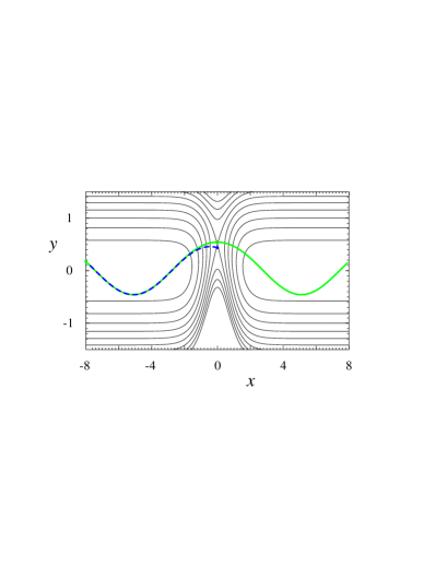
Figure 1: Contours of the model potential are shown for the case $\Omega=1$ and $\lambda=\mu=1/2$. The continuous line shows a real trajectory which is an extension of the complex periodic orbit (or instanton) used in the next section to construct the simplest semiclassical approximation. The dashed curve shows the trajectory defined by the decoupled dynamics of $V_{\infty}(y)$ to which it asymptotes.

For future reference, it will be useful to denote the asymptotically decoupled potential by the symbol

$$V(x,y)\sim V_{\infty}(y)=\frac{1}{2}\Omega^{2}y^{2}.$$

We can therefore write the asymptotic scattering states for this problem analytically, as solutions of a harmonic oscillator.

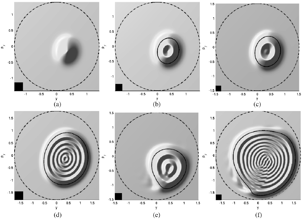
Figure 2: The Weyl symbol ${\cal W}_{{\hat{\cal R}}}(\mbox{\boldmath$\zeta$\unboldmath},E)$ is shown for the potential in (1). Cases (a) to (d) have $\Omega=1$ and $\lambda=\mu=1/2$ and energies (a) $E=1.0$, (b) $E=1.10$, (c) $E=1.15$ and (d) $E=1.6$. Cases (e) and (f) have $\Omega=1$, $\lambda=-1/2$ and $\mu=1$ and energies $E=1.15$ and $E=1.6$ respectively. Also shown are, the boundary of the allowed region as a dashed curve and, in cases (b) to (f) where the energy is above threshold, the boundary of the classically reacting region. In each case a box of area $\hbar$ is shown on the bottom left.

We write the scattering matrix in block form

$$S(E)=\left(\begin{matrix}r_{RR}&t_{RP}\\ t_{PR}&r_{PP}\end{matrix}\right),$$

where the subscripts $R$ and $P$ refer to reactant and product channels respectively. For example, the transmission matrix $t_{PR}$ maps asymptotically incoming states on the reactant side to asymptotically outgoing states on the product side. The theory we describe is for the matrix

$$\hat{\mathcal{R}}(E)=t_{PR}^{\dagger}t_{PR}$$

rather than for the scattering matrix itself. The matrix ${\hat{\cal R}}(E)$ has an obvious physical role determining state-specific reaction rates. The transmission probability for an incoming state labelled $|{\psi_{n}}\rangle$ on the reactant side can be written as a matrix element

$$p_{n}=\langle{\psi_{n}}|{{\hat{\cal R}}(E)}|{\psi_{n}}\rangle$$ (2)

of ${\hat{\cal R}}(E)$. In going from the scattering matrix to ${\hat{\cal R}}(E)$ we lose information about phase and about the distribution of product states but, as described in sC04 , uniform semiclassical approximations for ${\hat{\cal R}}(E)$ are expected to be considerably simpler than those for $S(E)$.

Formally, we can think of ${\hat{\cal R}}(E)$ as an operator acting on the Hilbert space ${\cal H}_{R}^{\rm in}(E)$ of asymptotically propagating states in the incoming reactant channel — in this context we refer to it as the reaction operator in the following. We consider systems for which there are a finite number $M$ of such states so ${\cal H}_{R}^{\rm in}(E)$ is finite-dimensional and ${\hat{\cal R}}(E)$ can be represented by an $M\times M$ matrix. The Wigner-Weyl correspondence offers an alternative representation as a function on phase space and the theory we outline in the coming sections is stated in those terms. In the remainder of this section we describe how the connection is made formally between the matrix representation and the representation in Wigner-Weyl correspondence, or the Weyl symbol of ${\hat{\cal R}}(E)$. In preparation for that discussion, let us first describe the phase space on which these representations are defined.

As described in sc05 (see also Bog ), the natural classical analog of the Hilbert space ${\cal H}_{R}^{\rm in}(E)$ is a Poincaré section $\Sigma_{R}^{\rm in}(E)$ defined by fixing the energy $E$ and an asymptotically large value of the reaction coordinate $x$. We use $(y,p_{y})$ as canonical coordinates on $\Sigma_{R}^{\rm in}(E)$ and we may alternatively denote points in $\Sigma_{R}^{\rm in}(E)$ using the vector notation

$$\mbox{\boldmath$\zeta$\unboldmath}=\left(\begin{array}[]{c}{y}\\ {p_{y}}\end{array}\right).$$

We define the allowed region of the $y$-$p_{y}$ plane by the condition $p_{y}^{2}/2+V_{\infty}(y)<E$ and note that, as usual in this sort of correspondence, the dimension $M$ of ${\cal H}_{R}^{\rm in}(E)$ is approximated by the Liouville area of this region divided by $2\pi\hbar$.

To calculate the Weyl symbol ${\cal W}_{{\hat{\cal R}}}(\mbox{\boldmath$\zeta$\unboldmath},E)$ of ${\hat{\cal R}}(E)$, we denote its individual matrix elements by $R_{nm}(E)=\langle{\psi_{n}}|{{\hat{\cal R}}(E)}|{\psi_{m}}\rangle$ and write

$${\cal W}_{{\hat{\cal R}}}(\mbox{\boldmath$\zeta$\unboldmath},E)=2\pi\hbar\sum_{nm}R_{nm}(E){\cal W}_{nm}(\mbox{\boldmath$\zeta$\unboldmath})$$ (3)

where ${\cal W}_{nm}(\mbox{\boldmath$\zeta$\unboldmath})$ are the Weyl symbols of the projectors $|{\psi_{n}}\rangle\langle{\psi_{m}}|/2\pi\hbar$ (the factors of $2\pi\hbar$ are to keep the notation consistent with standard practice for Wigner functions in the case $n=m$). For the asymptotically harmonic potential in (1) the functions ${\cal W}_{nm}(\mbox{\boldmath$\zeta$\unboldmath})$ are known analytically (see Ripamonti for example).

The Weyl symbol ${\cal W}_{{\hat{\cal R}}}(\mbox{\boldmath$\zeta$\unboldmath},E)$ of ${\hat{\cal R}}(E)$ provides a remarkably transparent means of visualising the quantum transmission problem and of relating the scattering matrix to the geometry of classical phase space. To illustrate, we show examples of ${\cal W}_{{\hat{\cal R}}}(\mbox{\boldmath$\zeta$\unboldmath},E)$ in Figure 2 for the model potential in (1) with energies at and above threshold. These results have been obtained by first computing the scattering matrix numerically using symplectic integration combined with the log derivative method as described in dM86 ; dM95 and then using (3). In each case we see that ${\cal W}_{{\hat{\cal R}}}(\mbox{\boldmath$\zeta$\unboldmath},E)$ is effectively supported in a region of $\Sigma_{R}^{\rm in}(E)$, which we can identify as the quantum-mechanically reacting region. Indeed, by rewriting the reaction probability in (2) (using standard properties of the Wigner-Weyl correspondence) in the form

$$p_{n}=\int{\cal W}_{{\hat{\cal R}}}(\mbox{\boldmath$\zeta$\unboldmath},E){\cal W}_{nn}(\mbox{\boldmath$\zeta$\unboldmath}){\rm d}\mbox{\boldmath$\zeta$\unboldmath},$$ (4)

where ${\rm d}\mbox{\boldmath$\zeta$\unboldmath}={\rm d}y{\rm d}p_{y}$, and interpreting the Wigner function ${\cal W}_{nn}(\mbox{\boldmath$\zeta$\unboldmath})$ as a phase space pseudodensity, it is natural to identify ${\cal W}_{{\hat{\cal R}}}(\mbox{\boldmath$\zeta$\unboldmath},E)$ as a probabability of reaction as a function of phase space, albeit in an averaged sense. Although the uncertainty principle prevents us from defining a point-wise transmission probability in phase space, we can construct linear combinations of incoming states with a fixed total energy (as in (5) below) whose Wigner function is supported within an area of $O(\hbar)$ in $\Sigma_{R}^{\rm in}(E)$ and the appropriate modification of (4) then gives the reaction probability as an average of ${\cal W}_{\hat{\cal R}}(\mbox{\boldmath$\zeta$\unboldmath},E)$ over that support.

For energies at or below threshold, transmission is controlled by tunnelling and ${\cal W}_{{\hat{\cal R}}}(\mbox{\boldmath$\zeta$\unboldmath},E)$ is supported in a phase space region of area $O(\hbar)$, centred around an initial condition that leads to an optimal tunnelling route. An explicit semiclassical expression for ${\cal W}_{{\hat{\cal R}}}(\mbox{\boldmath$\zeta$\unboldmath},E)$ in this case will be given later and one can see for the threshold case in Figure 2(a) that ${\cal W}_{{\hat{\cal R}}}(\mbox{\boldmath$\zeta$\unboldmath},E)$ is indeed peaked around a single point in $\Sigma_{R}^{\rm in}(E)$. As the energy increases above threshold, a classically reacting region appears, initially centred on the orbit associated with optimal tunnelling. The boundaries of the classically reacting regions are indicated in Figures 2(b) to (f) by continuous closed curves (as the energy falls to the threshold case $E=1$, the classically reacting region shrinks to a point corresponding to the optimal tunnelling route and around which ${\cal W}_{{\hat{\cal R}}}(\mbox{\boldmath$\zeta$\unboldmath},E)$ is concentrated). One can see in each case that the reacting region closely matches the support of ${\cal W}_{{\hat{\cal R}}}(\mbox{\boldmath$\zeta$\unboldmath},E)$.

Before describing how ${\cal W}_{{\hat{\cal R}}}(\mbox{\boldmath$\zeta$\unboldmath},E)$ is approximated semiclassically, we should outline how the classically reacting regions in Figure 2 are defined. The boundary of the classically reacting region in full phase space is the stable manifold on the reacting side of a PODS in two dimensions or more generally a NHIM if higher-dimensional problems are treated. Extended into the incoming reactant channel, this stable manifold defines a tube, the interior of which consists of classically reacting trajectories and whose annular exterior in the classically allowed region consists of trajectories which eventually return along the outgoing reactant channel. A representation of this reacting region in a Poincaré section $\Sigma_{R}^{\rm in}$ is obtained simply by taking the a section of the tube of reacting trajectories at fixed energy and a fixed, asymptotically large value of the reaction coordinate $x$. Since the tube continues to evolve asymptotically (according to the dynamics of a decoupled potential $V_{\infty}(y)$), the shape of a reacting region defined in this way will depend on the value chosen for the coordinate $x$. In models where the dynamics of the reacting region is nonlinear — or potentially even chaotic in problems of higher dimension — the shape of the reacting region will not have a limit and becomes ever more complicated as $x$ is brought to infinity. To obtain a fixed asymptotic limit we therefore renormalise the dynamics by using the decoupled evolution of the limiting potential $V_{\infty}(y)$ to map the asymptotic section back to one corresponding to a fixed finite value of $x$. In making semiclassical comparisons the value of $x$ used to define this final section is dictated by the conventions used for the scattering matrix.

In the present case the asymptotic states in terms of which the scattering matrix is defined are of the form,

$$\Psi_{n,E}(x,y)\sim\frac{{\rm e}^{ik_{n}x}}{\sqrt{\hbar k_{n}}}\psi_{n}(y),$$ (5)

where $\psi_{n}(y)$ are the eigenfunctions of the decoupled potential $V_{\infty}(y)$. The phases of these scattering states are zeroed at $x=0$ and asymptotic incoming states can be constructed by starting with the transverse modes at $x=0$ and propagating them backwards into the asymptotic region of the incoming channel using dynamics defined by $V_{\infty}(y)$. To make a comparison with the classical picture, the renormalisation of the classical dynamics should therefore take an asymptotic Poincaré section back to one defined by $x=0$. This is the convention used in Figure 2 to compare ${{\cal W}}_{{\hat{\cal R}}}(\mbox{\boldmath$\zeta$\unboldmath},E)$ with the classically reacting region. Alternative phase conventions would lead to a reaction operator ${\hat{\cal R}}(E)$ obtained by conjugation of the one we define by a unitary matrix which is diagonal in the basis $|{\psi_{n}}\rangle$. This conjugation makes no difference to the diagonal matrix elements $\langle{\psi_{n}}|{{\hat{\cal R}}}|{\psi_{n}}\rangle$ but is important for the appearance of the Weyl symbol in $\Sigma_{R}^{\rm in}$. Choosing values other than $x=0$ for the reference section $\Sigma_{R}^{\rm in}$ would, for example, lead to a deformation of the Weyl symbol by the asymptotically decoupled dynamics.

Note that this renormalisation procedure is simply means of interpreting a term in the phase function in the classical $S$-matrix MillerSmatrix that fixes its asymptotic value. By accounting for this term using a conjugation of the asymptotic dynamics by the mapping in decoupled dynamics back to $x=0$, we can incorporate everything about the classical $S$-matrix into a single Poincaré mapping and present results in a more compact form, as described more fully in the coming sections.

III Harmonic Approximation

In this section we describe a semiclassical approximation for ${\hat{\cal R}}(E)$ based on dynamics linearised around an optimal tunnelling orbit. Although less accurate and valid over a smaller range of energies than the fully nonlinear theory described in the next section, this harmonic approximation captures the essential qualitative behaviour of ${\hat{\cal R}}(E)$ and works well in the especially interesting range of energies around threshold where classical reaction switches on. It is also considerably simpler to apply and can be expressed in closed form using easily obtained classical data. Note that the term “harmonic” here refers simply to the fact that linearised dynamics about a tunnelling orbit are used and has nothing to do with the harmonic asymptotic behaviour of the model we use for numerical illustration.

III.1 Operator version

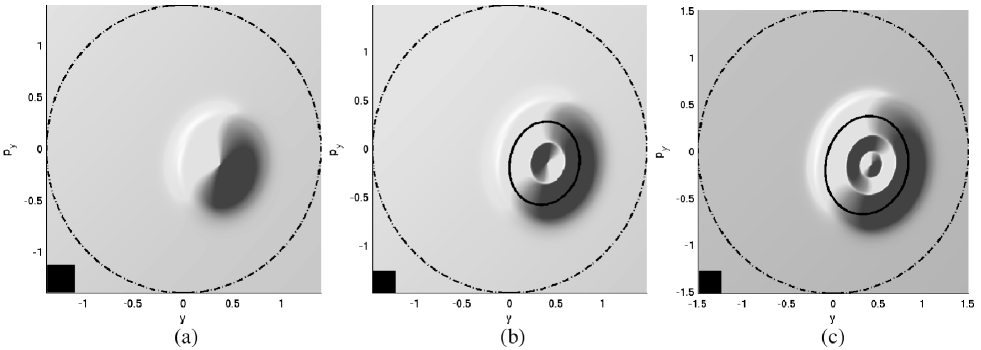
Figure 3: The harmonic approximation to ${\cal W}_{\hat{\cal R}}(\mbox{\boldmath$\zeta$\unboldmath},E)$ is shown for energies (a) $E=1$, (b) $E=1.10$ and (c) $E=1.15$, corresponding to the top row in Figure 2

A full description of the harmonic approximation to ${\hat{\cal R}}(E)$ has been given in sC04 and we refer there for details and a derivation of the approach. Here we simply summarise the important points. The operator ${\hat{\cal R}}(E)$ is approximated by a formula

$$\hat{\mathcal{R}}(E)\approx\frac{\hat{\mathcal{T}(E)}}{1+\hat{\mathcal{T}(E)}}$$ (6)

where ${\hat{\cal T}}(E)$ is a “tunnelling operator” constructed from classical data. The elements needed to compute ${\hat{\cal T}}(E)$ are as follows.

• A complex periodic orbit $\gamma_{E}(t)$, the “instanton”, is found which encircles the transition state in imaginary time. This orbit can be found for energies above and below threshold and its dynamical characteristics depend smoothly on energy there.

• At the end of the previous section it was described how the boundary of the reacting region can be first extended arbitrarily far into the asymptotic region and then renormalised by mapping back to a section $\Sigma_{R}^{\rm in}$ at $x=0$ using decoupled dynamics, so that the shape remains fixed as dynamics are extended into the asymptotic region. An analogous renormalisation, illustrated in Figure 2, is applied to $\gamma_{E}(t)$ so that an asymptotically fixed initial condtion for it is defined in $\Sigma_{R}^{\rm in}$. Above threshold this initial condition is near the centre of the reacting region.

• The imaginary action of $\gamma_{E}(t)$ is denoted $iK_{0}=\oint_{\gamma_{E}}{\bf p}\cdot{\rm d}{\bf q}$. We also denote $\theta=K_{0}/\hbar$. Note that for energies above threshold we have $K_{0}<0$ while $K_{0}>0$ below threshold.

• Linearised dynamics around $\gamma_{E}(t)$ are characterised by a complex monodromy matrix $W$, which is routinely determined as part of a numerical search for the orbit $\gamma_{E}(t)$. The eigenvalues of $W$ come in real reciprocal pairs $(\Lambda,\Lambda^{-1})$, which we order so that $\Lambda>1$.

• The matrix $W$ can be generated by using an elliptic quadratic Hamiltonian $h(\mbox{\boldmath$\zeta$\unboldmath})$ for an imaginary time $-i\tau_{0}$. Note that this Hamiltonian generates renormalised dynamics in the section $\Sigma_{R}^{\rm in}$ and is therefore not simply a truncation of the full Hamiltonian in the transition state region.

• Canonical coordinates $(Q,P)$ are defined on $\Sigma_{R}^{\rm in}$ so that

  $$h(\mbox{\boldmath$\zeta$\unboldmath})=\frac{\alpha}{2}\left(Q^{2}+P^{2}\right)$$

  and we have $\Lambda={\rm e}^{\alpha\tau_{0}}$.

The quantum analog of the classical generating Hamiltonian $h(\mbox{\boldmath$\zeta$\unboldmath})$ is denoted by $\hat{h}$.

We can now write the tunnelling operator ${\hat{\cal T}}(E)$ in the form

$${\hat{\cal T}}={\rm e}^{-\theta-\tau_{0}\hat{h}/\hbar},$$ (7)

which, except for the prefactor ${\rm e}^{-\theta}$, is an imaginary-time evolution operator generated by $\hat{h}$. Since $\hat{h}$ is harmonic we can explicitly construct its eigenstates $|{\varphi_{k}}\rangle$, with $k=0,1,\cdots$ and the corresponding eigensolutions of ${\hat{\cal T}}$ are

$${\hat{\cal T}}|{\varphi_{k}}\rangle=\tau_{k}|{\varphi_{k}}\rangle$$

where the eigenvalues

$$\tau_{k}={\rm e}^{-\theta}\Lambda^{-(k+\frac{1}{2})}$$ (8)

are deduced simply by exponentiating the eigenvalues of $\hat{h}$.

III.2 Weyl symbol

It is shown in sC04 how closed form approximations can be deduced for phase space representations of ${\hat{\cal R}}(E)$ as a result of substituting this exponentiated form for ${\hat{\cal T}}(E)$ in (6) and resumming the geometric series ${\hat{\cal R}}={\hat{\cal T}}-{\hat{\cal T}}^{2}+{\hat{\cal T}}^{3}-\cdots$. This leads to an integral representation

$${\hat{\cal R}}(E)=\frac{1}{2i}\int_{C}\frac{{\rm e}^{-\rho(\theta+\tau_{0}\hat{h}/\hbar)}}{\sin\pi\rho}{\rm d}\rho$$ (9)

for ${\hat{\cal R}}(E)$, in which the contour $C$ ascends just to the right of the imaginary axis. Standard asymptotic approaches to this integral, such as the method of steepest descent, allow explicit asymptotic approximations to be written for ${\hat{\cal R}}$ in various representations, including for the Weyl symbol.

These expressions are especially useful to understand the detailed structure of ${\hat{\cal R}}(E)$ in phase space, but for the purposes of computing ${\hat{\cal R}}(E)$ for the parameter regimes we consider here, it suffices to use an an eigenexpansion

$$\hat{\mathcal{R}}(E)\approx\sum_{k}r_{k}|{\varphi_{k}}\rangle\langle{\varphi_{k}}|$$ (10)

where

$$r_{k}=\frac{\tau_{k}}{1+\tau_{k}}.$$ (11)

The Weyl symbol of ${\hat{\cal R}}(E)$ can, for example, be written as

$${\cal W}_{{\hat{\cal R}}}(\mbox{\boldmath$\zeta$\unboldmath},E)\approx 2\pi\hbar\sum_{k}r_{k}(E)\tilde{{\cal W}}_{kk}(\mbox{\boldmath$\zeta$\unboldmath})$$

where $\tilde{{\cal W}}_{kk}(\mbox{\boldmath$\zeta$\unboldmath})$ are the Wigner functions of the states $|{\varphi_{k}}\rangle$ (and given analytically in Ripamonti for example). The tilde distinguishes these Wigner functions from those of the basis states $|{\psi_{n}}\rangle$ of the scattering operator, which are different.

The canonical coordinates $(Q,P)$ are centred on the initial condition for $\gamma_{E}(t)$ in $\Sigma_{R}^{\rm in}$ and are such that for energies just above threshold, the classically reacting region is circular in the $(Q,P)$ plane. In the original coordinate system $(y,p_{y})$ these Wigner functions are translated, squeezed and rotated so that their level curves are aligned with the approximately elliptical reacting region. The resulting approximation for ${\cal W}_{{\hat{\cal R}}}(\mbox{\boldmath$\zeta$\unboldmath},E)$ therefore describes an elliptically-shaped representation of the true quantum transmission problem

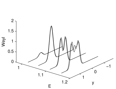
Figure 4: The harmonic approximation is compared with exact results for ${\cal W}_{\hat{\cal R}}(\mbox{\boldmath$\zeta$\unboldmath},E)$ at energies at and just above threshold. These are obtained by sampling ${\cal W}_{\hat{\cal R}}(\mbox{\boldmath$\zeta$\unboldmath},E)$ along a horizontal line through the centre of the reacting region in $\Sigma_{R}^{\rm in}$ and plotting the result as a function of $y$. Parameters in the potential are as in Figures 2(a)-(d) and 3.

The harmonically approximated Weyl symbol ${\cal W}_{{\hat{\cal R}}}(\mbox{\boldmath$\zeta$\unboldmath},E)$ is illustrated in Figure 3 for three energies at and just above threshold in the model potential with $\Omega=1$ and $\lambda=1/2=\mu$. For comparison, illustrations of corresponding exact calculations can be found in the top row of Figure 2. In general we find that the harmonic approximation is in good quantitative agreement with exact results at and below threshold. The threshold case in Figure 3(a), for example, is indistinguishable from the corresponding exact result in Figure 2(a) at the level of graphical resolution used. As energy increases, the agreement deteriorates so that noticable differences are visible when $E=1.15$ (harmonic approximation in Figure 3(c) and exact calculation in Figure 2(c)). It should be emphasised, however, that even then, the harmonic approximation captures the essential qualitative features of ${\cal W}_{{\hat{\cal R}}}(\mbox{\boldmath$\zeta$\unboldmath},E)$.

In order to make a closer comparison between exact and harmonic results, we show one-dimensional sections through the Weyl symbol in Figure 4. In each case ${\cal W}_{{\hat{\cal R}}}(\mbox{\boldmath$\zeta$\unboldmath},E)$ is sampled along a horizontal line through the centre of the reacting region in $\Sigma_{R}^{\rm in}$ and plotted as a function of the $y$ coordinate. There is good quantitative agreement in cases (a) and (b) where the enrgy is at and just above threshold. At higher energies the harmonic approximation captures the support of the quantum-mechanically reacting region well but details of the Wigner function do not match at the centre of the reacting region. It should be remarked, however, that oscillations in the Weyl symbol are sensitive to nonlocal changes in phase space and discrepencies at the centre of the reacting region may not have a strong effect on averaged reaction probabilities as expressed in (4).

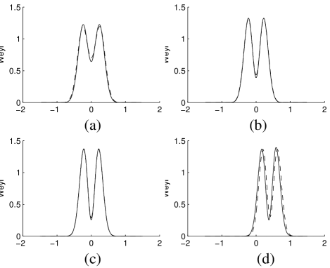
Figure 5: The harmonic and exact Weyl symbols are compared for different potentials with $\Omega=1$ and (a) $\lambda=-{1\over 2}$, $\mu=0$; (b) $\lambda=0$, $\mu=0$; (c) $\lambda={1\over 2}$, $\mu=0$; (d) $\lambda={1\over 2}$, $\mu={1\over 2}$. In each case the energy is chosen so that the classically reactive flux has the fixed value $N_{\rm cl}(E)=2$.

Similar one-dimensional sections are shown in Figure 5 which illustrate the harmonic approximation for different parameter sets. In each of these the energy is chosen so that the cumulative reactive flux

$$N_{\rm cl}(E)=\frac{1}{2\pi\hbar}\oint_{\rm PODS}{\bf p}\cdot{\rm d}{\bf q}=\frac{E-1}{\hbar\sqrt{\Omega^{2}+\lambda}}$$

is fixed (at the value 2). Figures 5(a), (b) and (c) show cases where $\mu=0$ and the potential has a symmetry in $y$. Figure 5(a) has a negative value of $\lambda=-1/2$ for which an adiabatic approximation assuming fast transverse dynamics in the barrier region would not be expected to apply. Figure 5(b) is the separable case $\lambda=0$ and in Figure 5(c) we have $\lambda=1/2$. Note that separability does not confer a particular computational advantage in this approach, nor does it lead to particularly better accuracy of the approximation. In Figure 5(d), an example is shown in which $\mu=1/2$ and the potential is neither separable nor symmetric in $y$. The approximation works less well in that case. This is not unexpected because corrections to the harmonic approximation will be quartic rather than cubic in a symmetric problem but we note that there is still good agreement.

IV Non-Linear Approximation

Although the harmonic approximation captures the essential qualitative features of quantum transmission and works well quantitatively near threshold, we can achieve greater range of applicability and significantly improved numerical agreement if we use fully nonlinear dynamics around the orbit $\gamma_{E}(t)$. The price to be paid for this improvement is that the resulting calculation is significantly more involved. The greatest impediment is that, although the tunnelling operator defined by nonlinear evolution can be routinely approximated semiclassically, we do not know at present how to write semiclassical approximations for the operator $(1+{\hat{\cal T}})^{-1}$ directly in terms of classical orbits. In this paper we simply use numerical inversion of the matrix representation of $1+{\hat{\cal T}}$. Before describing this procedure, it is helpful to describe how nonlinear calculation is incorporated in the operator ${\hat{\cal T}}$. This is done in section IV.1 below, followed by a description of the uniform calculation in section IV.2.

IV.1 Primitive approximation

At energies below threshold the imaginary action of the orbit $\gamma_{E}(t)$ is positive, that is $\theta>0$, and the exponential prefactor ${\rm e}^{-\theta}$ in (7) makes ${\hat{\cal T}}$ small. We may therefore approximate the reaction operator directly by the tunnelling operator, giving

$${\hat{\cal R}}(E)\approx{\hat{\cal T}}(E),$$

which we refer to as the primitive approximation. The primitive approximation is easily extended beyond the immediate neighbourhood of $\gamma_{E}(t)$. Instead of letting ${\hat{\cal T}}$ be the evolution operator corresponding to the classically linear evolution defined by $W$, as we did in the previous section, we let it be the quantum version of a nonlinear map in $\Sigma_{R}^{\rm in}$.

Initial conditions near $\gamma_{E}(t)$ in $\Sigma_{R}^{\rm in}$ can be followed over a sequence of time evolutions similar to those of $\gamma_{E}(t)$ itself until they return to $\Sigma_{R}^{\rm in}$, defining a surface-of-section mapping which we denote by

$${\cal F}:\Sigma_{R}^{\rm in}\to\Sigma_{R}^{\rm in}.$$

As with conventional return maps, ${\cal F}$ defines a canonical transformation on $\Sigma_{R}^{\rm in}$, except that it is complex, in general taking real initial conditions to complex images. Despite this complexity, the evolution has a quantum analog as an evolution operator, and this is the tunnelling operator ${\hat{\cal T}}$.

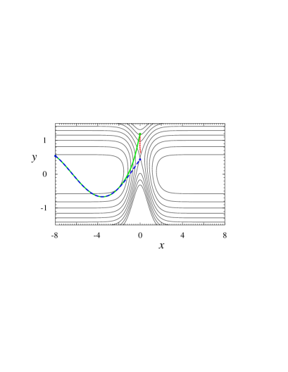
Figure 6: The projection onto real configuration space of a typical midpoint orbit is shown. This orbit can be obtained by continuously deforming the initial conditions for the orbit shown in Figure 1. The dotted segment corresponds to evolution over the imaginary part of the time contour and the dashed segment corresponds to renormalisation by the uncoupled dynamics. The symmetry $\mbox{\boldmath$\zeta$\unboldmath}_{B}=\mbox{\boldmath$\zeta$\unboldmath}_{A}^{*}$ means that the real part of the orbit shown here is self-retracing, with the orbit turning back on itself at the end of the dotted segment.

With suitable modifications to take account of the complexity of the mapping, standard semiclassical approximations that are applied to evolution operators, such as the Van Vleck formula, can be used to approximate ${\hat{\cal T}}$. Here we focus on an approximation derived in mB89 for the Weyl symbol of an operator (see also sC99 ). For the Weyl symbol of the operator ${\hat{\cal T}}$ we write

$${\cal W}_{{\hat{\cal T}}}(\mbox{\boldmath$\zeta$\unboldmath},E)\approx\frac{{\rm e}^{-\mathcal{A}(\bm{\zeta},E)/\hbar}}{\sqrt{{\rm det}\,(W_{AB}+I)/2}},$$ (12)

where ${\cal{A}}$ and $W_{AB}$ are calculated from a midpoint orbit $\mbox{\boldmath$\zeta$\unboldmath}_{A}\to\mbox{\boldmath$\zeta$\unboldmath}_{B}$ which is defined by the conditions

$$\zeta = {1\over 2}\left(\mbox{\boldmath$\zeta$\unboldmath}_{A}+\mbox{\boldmath$\zeta$\unboldmath}_{B}\right)$$

$$\mbox{\boldmath$\zeta$\unboldmath}_{B} = {\cal F}(\mbox{\boldmath$\zeta$\unboldmath}_{A}).$$ (13)

That is, the point $\zeta$ at which the Weyl symbol is to be evaluated is the midpoint of $\mbox{\boldmath$\zeta$\unboldmath}_{A}$ and $\mbox{\boldmath$\zeta$\unboldmath}_{B}$, where $\mbox{\boldmath$\zeta$\unboldmath}_{A}$ evolves into $\mbox{\boldmath$\zeta$\unboldmath}_{B}$ under the return map. The exponent ${\cal{A}}(\mbox{\boldmath$\zeta$\unboldmath},E)$ is such that

$$i{\cal{A}}(\mbox{\boldmath$\zeta$\unboldmath},E)=\int_{\mbox{\boldmath$\zeta$\unboldmath}_{A}}^{\mbox{\boldmath$\zeta$\unboldmath}_{B}}{\bf p}\cdot{\rm d}{\bf q}-p_{y}(y_{B}-y_{A})$$

and the matrix $W_{AB}$ is a linearisation the map ${\cal F}$ around the orbit $\mbox{\boldmath$\zeta$\unboldmath}_{A}\to\mbox{\boldmath$\zeta$\unboldmath}_{B}$.

It can be shown sc05 that the complex conjugate of the map ${\cal F}$ is its inverse, ${\cal F}^{*}={\cal F}^{-1}$, and from this a number of important symmetries follow which guarantee that ${\cal W}_{{\hat{\cal T}}}(\mbox{\boldmath$\zeta$\unboldmath},E)$ is a real-valued function on $\Sigma_{R}^{\rm in}$ that is peaked around the initial condition for $\gamma_{E}(t)$, which we denote by $\mbox{\boldmath$\zeta$\unboldmath}_{0}$ in the following. On a formal level, the real-valuedness of ${\cal W}_{{\hat{\cal T}}}(\mbox{\boldmath$\zeta$\unboldmath},E)$ follows from the observation that ${\hat{\cal T}}$ is Hermitian which, as discussed in sC99 , is a quantum analog of the property ${\cal F}^{*}={\cal F}^{-1}$. It is instructive, however, to see how the real-valuedness of the semiclassical approximation to ${\cal W}_{{\hat{\cal T}}}(\mbox{\boldmath$\zeta$\unboldmath},E)$ follows directly from the symmetries of the midpoint orbit.

First we note that, given a midpoint orbit $\mbox{\boldmath$\zeta$\unboldmath}_{A}\to\mbox{\boldmath$\zeta$\unboldmath}_{B}$ for a real-valued $\zeta$, then $\mbox{\boldmath$\zeta$\unboldmath}_{B}^{*}\to\mbox{\boldmath$\zeta$\unboldmath}_{A}^{*}$ is also a midpoint orbit (for the same $\zeta$). This can be seen by conjugating the relations in (IV.1) and using $\mbox{\boldmath$\zeta$\unboldmath}_{B}^{*}=[({\cal F}(\mbox{\boldmath$\zeta$\unboldmath}_{A})]^{*}={\cal F}^{*}(\mbox{\boldmath$\zeta$\unboldmath}_{A}^{*})={\cal F}^{-1}(\mbox{\boldmath$\zeta$\unboldmath}_{A}^{*})$ to deduce that $\mbox{\boldmath$\zeta$\unboldmath}_{A}^{*}={\cal F}(\mbox{\boldmath$\zeta$\unboldmath}_{B}^{*})$. It turns out in fact that these two midpoint orbits coincide, so

$$\mbox{\boldmath$\zeta$\unboldmath}_{B}=\mbox{\boldmath$\zeta$\unboldmath}_{A}^{*}$$

and

$${\rm Re}\,\mbox{\boldmath$\zeta$\unboldmath}_{B}=\mbox{\boldmath$\zeta$\unboldmath}={\rm Re}\,\mbox{\boldmath$\zeta$\unboldmath}_{A}.$$

This is easily confirmed for the linearised map (replacing ${\cal F}$ by multiplication by $W$ and using $W^{*}=W^{-1}$) and therefore holds for the nonlinear map if $\zeta$ is close enough to $\mbox{\boldmath$\zeta$\unboldmath}_{0}$. The condition $\mbox{\boldmath$\zeta$\unboldmath}_{B}=\mbox{\boldmath$\zeta$\unboldmath}_{A}^{*}$ can only be violated if a bifurcation is encountered and a more detailed analysis shows that this corresponds to the condition ${\rm det}\,(W_{AB}+I)=0$, which would lead to a caustic in (12). We will assume in this paper that no such caustics are encountered in the region of $\Sigma_{R}^{\rm in}$ which dominates reaction.

An example of a full trajectory corresponding to a typical midpoint orbit is illustrated in Figure 6. Because the initial conditions are complex, the coordinates of the trajectory are generically complex over its length, even along the segments which have been obtained by deformation of the real segments of $\gamma_{E}(t)$. A consequence of the symmetry $\mbox{\boldmath$\zeta$\unboldmath}_{B}=\mbox{\boldmath$\zeta$\unboldmath}_{A}^{*}$, however, is that the time contours can be chosen so that the second half of the trajectory reverses the complex conjugate of the first half. A projection onto real configuration space, for example, is self retracing. We find as a result that the action is purely imaginary and the exponent ${\cal{A}}(\mbox{\boldmath$\zeta$\unboldmath},E)$ is a positive real number. We also find that $W_{AB}^{*}=W_{AB}^{-1}$ and because ${\rm det}\,W_{AB}=1$ this means that the amplitude term ${\rm det}\,(W_{AB}+I)$ in (12) is real (and positive). Therefore ${\cal W}_{{\hat{\cal T}}}(\mbox{\boldmath$\zeta$\unboldmath},E)$ is a positive real-valued function with a maximum at $\mbox{\boldmath$\zeta$\unboldmath}_{0}$ (for which we have ${\cal{A}}(\mbox{\boldmath$\zeta$\unboldmath}_{0},E)=K_{0}(E)$).

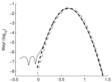
Figure 7: For an energy $E=0.985$ just below threshold, a comparison is given on a logarithmic scale between the exact Weyl symbol (continuous curve), the nonlinear primitive approximation of Equation (12) (heavy dashed curve) and the harmonic primitive approximation of Equation (14) (light dashed curve). The parameters here are $\Omega=1$, $\lambda=-1/2$, and $\mu=1$. The nonlinear primitive result works well over a large region of phase space but does not capture the oscillations in the tail of the exact calculation, which may well be a signature of nonintegrable complex-dynamical effects of the type described in aY00 ; Takahashi ; TYK

The harmonic approximation can be recovered by expanding the exponent to second order about $\mbox{\boldmath$\zeta$\unboldmath}_{0}$ and approximating $W_{AB}$ by $W$, giving sC04

$${\cal W}_{\hat{\cal T}}(\mbox{\boldmath$\zeta$\unboldmath},E)\approx\frac{{\rm e}^{-\theta-[(2/\beta)\tanh\beta/2]\tau_{0}h(\mbox{\boldmath$\scriptstyle\zeta$\unboldmath})/\hbar}}{\cosh\beta/2}.$$ (14)

A comparison is given in Figure 7 between this approximation, the fully nonlinear approximation of (12) and exact results. Although the harmonic approximation works well near the maximum of the Weyl symbol, the fully nonlinear result works better over a larger range. We note however that there is qualitative deviation even from the nonlinear approximation in the deep tunnelling regime where the exact calculation shows significant oscillations not captured by the harmonic or nonlinear approximations. Similar oscillatory structure, or “fringed tunnelling” in the scattering matrix has been explained in aY00 ; Takahashi ; TYK on the basis of nonintegrable complex dynamics and has been shown to involve mechanisms that also show up in chaotic tunnelling. It seems likely that the oscillations in Figure 7 have a similar origin but we have not preformed a detailed analysis. It will be an interesting problem in the future to combine the inherently nonintegrable mechanism in aY00 ; Takahashi ; TYK with the uniform approximations illustrated here.

IV.2 Uniform approximation

Although we now have an explicit closed-form semiclassical approximation for ${\hat{\cal T}}$, no equivalent result is currently available for the uniformisation ${\hat{\cal T}}/(1+{\hat{\cal T}})$ because inversion of the operator $1+{\hat{\cal T}}$ cannot be done simply. In this paper we simply adopt a hybrid approach which combines semiclassical approximation of ${\hat{\cal T}}$ with numerical inversion of $1+{\hat{\cal T}}$. Although not a fully semiclassical method, this will allow us to verify that (6) gives an accurate reproduction of quantum transmission.

We first represent ${\hat{\cal T}}$ as a matrix in the same asymptotic basis $|{\psi_{n}}\rangle$ as used for the scattering matrix. We denote individual matrix elements by $T_{nm}=\langle{\psi_{n}}|{{\hat{\cal T}}}|{\psi_{m}}\rangle$ and compute them using the Wigner-Weyl calculus by writing

$$T_{nm}(E)=\int{\cal W}_{nm}(\mbox{\boldmath$\zeta$\unboldmath}){\cal W}_{{\hat{\cal T}}}(\mbox{\boldmath$\zeta$\unboldmath},E){\rm d}\mbox{\boldmath$\zeta$\unboldmath}$$ (15)

and approximating ${\cal W}_{{\hat{\cal T}}}(\mbox{\boldmath$\zeta$\unboldmath},E)$ using (12). We emphasise that while ${\hat{\cal T}}$ is almost diagonal in the basis $|{\varphi_{k}}\rangle$ of eigenstates of the generating Hamiltonian $\hat{h}$, the same is not true in the basis $|{\psi_{n}}\rangle$ unless the potential is separable. The integral is performed numerically and the resulting $M\times M$ matrix for ${\hat{\cal T}}/(1+{\hat{\cal T}})$, whose elements are denoted $R_{nm}^{\rm sc}(E)$, is also computed numerically. This integration is not difficult since a grid on $\Sigma_{R}^{\rm in}$ is easily filled by using Newton integration to step the midpoint orbit, starting with the known solution corresponding to $\gamma_{E}(t)$ at $\mbox{\boldmath$\zeta$\unboldmath}_{0}$ (for which $\mbox{\boldmath$\zeta$\unboldmath}_{A}=\mbox{\boldmath$\zeta$\unboldmath}_{0}=\mbox{\boldmath$\zeta$\unboldmath}_{B}$). Once the elements $R_{nm}^{\rm sc}(E)$ are known, the Weyl symbol for ${\hat{\cal T}}/(1+{\hat{\cal T}})$ is obtained by replacing $R_{nm}(E)$ with $R_{nm}^{\rm sc}(E)$ in (3).

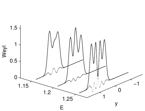
Figure 8: The uniform nonlinear approximation is compared with the exact Weyl symbol for a series of energies and the same parameters as used in Figure 4. It is difficult the distinguish the exact and approximate results at the level of graphical resolution used, but in each case the difference multiplied by $10$ is shown underneath as a dotted curve.

We find excellent agreement between the semiclassically computed Weyl symbol ${\cal W}_{{\hat{\cal R}}}(\mbox{\boldmath$\zeta$\unboldmath},E)$ and the exact result. A nonlinear version of Figure 3 is indistinguishable from the exact results shown in the top row of Figure 2 and therefore not shown. Instead we compare in Figure 8 horizontal slices of the Weyl symbol through the reacting region, in the same manner as in Figure 4. The potential used is the same as in Figure 4 and the energies treated extend somewhat higher above the threshold. The exact and semiclassical results cannot be distinguished at the resolution used, so the difference scaled by a factor of $10$ is also shown. We find similarly good agreement for other parameter sets we ahve investigated and we note that the quality of the approximation does not require special features of the classical dynamics such as symmetry, separability or adiabatic separation of transverse from reaction degrees of freedom.

We should remark that the current hybrid implementation of the nonlinear calculation is cumbersome and is harder to apply further above the barrier where the larger region of integration demands that we extend the midpoint trajectory deeper into complex phase space. We have not, for example, reproduced the results on the second row of Fig. 2 using this method. The purpose of this calculation is to show that the nonlinear uniform result derived in sc05 provides an accurate description of ${\hat{\cal R}}(E)$ in the model considered and that the method therefore deserves further exploration. Even though numerical inversion was used in applying the formalism, it is built entirely on a semiclassical approximation for the tunnelling operator ${\hat{\cal T}}(E)$ and we expect that any subsequent fully semiclassical implementation will be equally accurate.

We also remark that the current hybrid method is theoretically clumsy and obscures somewhat the deeper connections between the quantum results and the underlying classical geometry. For example, it would be especially interesting to characterise the behaviour of ${\cal W}_{\hat{\cal R}}(\mbox{\boldmath$\zeta$\unboldmath},E)$ at the boundary of the classically reacting region where trajectories approach the PODS (or NHIM in higher dimensions) along its stable manifold and where the classical reaction probability drops sharply from $1$ to $0$. Such an analytical approximation was found in sC04 for the harmonic version in which ${\cal W}_{\hat{\cal R}}(\mbox{\boldmath$\zeta$\unboldmath},E)$ is approximated as an integral of the Airy function near the boundary of classical reaction. Investigation is currently underway into a method to derive similar results in the nonlinear case on the basis of generating ${\hat{\cal T}}$ as in equation (7), but with an anharmonic generator $\hat{h}$ computed using classical normal form theory. Ultimately it should be possible to describe explicitly how the quantum reaction probability varies across the boundary of the classically reacting region in terms of trajectories which approach the complexified PODS along its stable manifold and evolve along it before returning to the asymptotic Poincaré section.

V Conclusions

We have successfully treated quantum transmission across a multidimensional barrier using uniform semiclassical approximation. The method applies generically around a threshold energy and does not rely on specific features of the classical dynamics such as separability or the existence of action angle variables. In its fully nonlinear incarnation the method gives an accurate description of reaction probabilities in phase space and makes a striking connection between the quantum scattering problem and the geometry of classical reaction. We expect that it will work equally well in higher-dimensional problems, even in cases where the incoming states are chaotic in the transverse dynamics.

Although we have shown that the fully nonlinear version works well, in doing so we have resorted to numerical methods which are not in the spirit of semiclassical approximation. The theory therefore needs further development in order to achieve a fully semiclassical description of the emerging reacting region. One promising approach which is currently under investigation is to use classical normal form theory to generate dynamics around the orbit $\gamma_{E}(t)$ using a nonlinear extension of the generator $h(\mbox{\boldmath$\zeta$\unboldmath})$. Many of the explicit analytical approaches used in the harmonic case might then be adapted to the nonlinear approximation. In particular this is expected to produce a detailed analytical description of the Weyl symbol at the boundary of the reacting region which calls on intrinsic geometrical features of (the stable manifold of) the NHIM.

A second aspect of the calculation which deserves further attention is the treatment of rotational degrees of freedom in fully three-dimensional models of chemical reaction. Although at one level this is simply a question of applying the results here individually to symmetry-reduced phase spaces for given angular momentum quantum numbers, there are interesting and nontrivial problems in describing the quantum-classical correspondence compactly in operator form. This is an especially interesting issue for reactions which proceed through a collinear mechanism since the collinear configurations are a singular part of the classical reduction process.

Acknowledgements
CSD is supported by an EPSRC studentship and SCC acknowledges support by the European Network MASIE, Contract No. HPRN-CT-2000-00113..

References

- (1) A. Shudo and K. S. Ikeda, Phys. Rev. Lett. 74, 682 (1995); Physica D 115, 234 (1998).
- (2) T. Onishi, A. Shudo, K. S. Ikeda and K. Takahashi, Phys. Rev. E 64, 025201(R) (2001).
- (3) A. Shudo, Y. Ishii and K. S. Ikeda, J. Phys. A 35, L225 (2002).
- (4) A. Yoshimoto, Rep. Maths. Phys. 46, 303 (2000).
- (5) K. Takahashi and K. S. Ikeda, Found. Phys. 31, 177 (2001); J. Phys. A 36, 7953 (2003).
- (6) K. Takahashi, A. Yoshimoto and K. S. Ikeda, Physics Letters A 297, 370 (2002).
- (7) S. C. Creagh, Nonlinearity 17, 1261 (2004).
- (8) S. C. Creagh, to appear in Nonlinearity. arXiv:nlin.CD/0506004
- (9) P. Pechukas, in Dynamics of Molecular Collisions, W. H. Miller (ed.) (New York: Plenum Press, 1976).
- (10) E. Pollak, M. S. Child and P. Pechukas, J. Chem. Phys. 72, 1669 (1979).
- (11) C. Jaffé, D. Farrelly and T. Uzer, Phys. Rev. A 60, 3833 (1999); Phys. Rev. Lett. 84, 610 (2000).
- (12) S Wiggins, L Wiesenfeld, C Jaffé and T Uzer Phys. Rev. Lett. 86, 5478 (2001); T. Uzer, C. Jaffé, J. Palacián, P. Yanguas and S. Wiggins, Nonlinearity 15, 957 (2002).
- (13) H Waalkens and S Wiggins, J. Phys. A 37, L435, (2004).
- (14) H Waalkens, A Burbanks and S Wiggins J. Chem. Phys. 121 6207, (2004).
- (15) L Wiesenfeld, J. Phys. A 37, L143, (2004).
- (16) W. H. Miller and T. F. George, J. Chem. Phys. 56, 5668 (1972); ibid. 57, 2458 (1972).
- (17) W. H. Miller, Adv. Chem. Phys. 25, 69 (1974); ibid. 30, 77 (1976).
- (18) K. W. Ford and J. A. Wheeler, Ann. Phys. 7, 259 (1959); ibid. 7 287 (1959).
- (19) M V Berry and K E Mount, Rep. Prog. Phys. 35, 315 (1972).
- (20) D. M. Brink and U. Smilanski, Nucl. Phys. A 405, 301 (1983).
- (21) W. H. Miller, J. Chem. Phys. 62, 1899 (1975); W H Miller, Faraday Discussions Chem. Soc. 62 40 (1977).
- (22) Y. Elran and K. G. Kay, J. Chem. Phys. 114, 4362 (2001); ibid. 116, 10577 (2002).
- (23) E. B. Bogomolny, Nonlinearity 5, 805 (1992).
- (24) N. Ripamonti, J. Phys. A 29, 5137 (1996).
- (25) D. E. Manolopoulos, J. Chem. Phys. 85, 6425 (1986).
- (26) D. E. Manolopoulos and S. K. Gray, J. Chem. Phys. 102, 9214 (1995).
- (27) M. V. Berry, Proc. R. Soc. Lond. A 423, 219 (1989).
- (28) S. C. Creagh and N. D. Whelan, Ann. Phys. 272, 196 (1999).