Uniform semiclassical trace formula for U(3) $\to$ SO(3) symmetry breaking

Abstract

We develop a uniform semiclassical trace formula for the density of states of a three-dimensional isotropic harmonic oscillator (HO), perturbed by a term $\frac{1}{4}\epsilon\,r^{4}$. This term breaks the U(3) symmetry of the HO, resulting in a spherical system with SO(3) symmetry. We first treat the anharmonic term for small $\epsilon$ in semiclassical perturbation theory by integration of the action of the perturbed periodic HO orbit families over the manifold $\mathbb{C}$P² which is covered by the parameters describing their four-fold degeneracy. Then we obtain an analytical uniform trace formula for arbitrary $\epsilon$ which in the limit of strong perturbations (or high energy) asymptotically goes over into the correct trace formula of the full anharmonic system with SO(3) symmetry, and in the limit $\epsilon$ (or energy) $\to 0$ restores the HO trace formula with U(3) symmetry. We demonstrate that the gross-shell structure of this anharmonically perturbed system is dominated by the two-fold degenerate diameter and circular orbits, and not by the orbits with the largest classical degeneracy, which are the three-fold degenerate tori with rational ratios $\omega_{r}:\omega_{\varphi}=N\!:\!M$ of radial and angular frequencies. The same holds also for the limit of a purely quartic spherical potential $V(r)\propto r^{4}$.

I Introduction

The semiclassical quantisation of non-integrable systems using properties of their periodic orbits was triggered by M. Gutzwiller gutz and extended by several groups bablo ; struma ; crli1 ; crli2 . It allows one to express the oscillating part $\delta g(E)$ of the quantum-mechanical density of states, given exactly in terms of a quantum spectrum $E_{n}$ and separated into two terms by

$$g(E)=\sum_{n}\delta(E-E_{n})={\widetilde{g}}\,(E)+\delta g(E)\,,$$ (1)

through a semiclassical trace formula of the form

$$\delta g_{sc}(E)\simeq\sum_{po}{\cal A}_{po}(E)\cos\,[S_{po}(E)/\hbar-\sigma_{po}\pi/2]\,.$$ (2)

The sum is over all periodic orbits $(po)$ of the classical system, $S_{po}(E)=\oint{\bf p}\cdot d{\bf q}$ are their action integrals, the amplitudes ${\cal A}_{po}(E)$ depend on their stabilities and degeneracies, and $\sigma_{po}$ are some phases called Maslov indices. The average part ${\widetilde{g}}\,(E)$ of the density of states, which by definition varies smoothly with energy, is obtained by the extended Thomas-Fermi (ETF) model (see, e.g., book , Chapter 4). Then, the sum $g_{ETF}(E)+\delta g_{sc}(E)$ usually turns out to be a good approximation to the exact quantity (1), although the sum over the $po$ in (2) is only an asymptotic one, correct to leading order in $1/\hbar$, and in chaotic systems is hampered by convergence problems chaos . For integrable systems, Berry and Tabor bertab and later Creagh et al. crli2 showed how a trace formula of the form (2) can quite generally be obtained from the Einstein-Brillouin-Keller (EBK) quantisation ebk . This method will be used in the present paper for a spherical system.

The semiclassical theory, often referred to as periodic orbit theory (POT), has been very successful not only in (partial) quantisation of a given Hamiltonian, but also in interpreting many experimentally observable quantum oscillations in finite fermion systems – so-called “shell effects” – in terms of classical mechanics. Examples are atomic nuclei bm , metallic clusters nish ; klavs ; mbclus , semiconductor quantum dots steffi , and metallic nanowires wire . An overview over many aspects of the POT and illustrative applications are given in book .

One problem that remains with all the trace formulae developed in the work quoted above is that the amplitudes ${\cal A}_{po}$ diverge in situations where a continuous symmetry is broken or restored under the variation of a system parameter (which may also be the energy $E$), or where bifurcations of periodic orbits occur. In such situations one has to go beyond the stationary phase approximation which is underlying the semiclassical approach. This has, besides bablo ; struma ; crli1 ; crli2 ; bertab , been developed most systematically by Ozorio de Almeida and Hannay ozoha for both situations, leading to local uniform approximations with finite amplitudes ${\cal A}_{po}$. So-called global uniform approximations, which yield finite amplitudes at symmetry-breaking and bifurcation points and far from them go over into the standard (extended) Gutzwiller trace formula, were developed for the breaking of U(1) symmetry in toms , for some cases of U(2) and SO(3) symmetry breaking in hhuni , and for various types of bifurcations in ssun . (Details and further references may be found in book , Chapter 6.3.)

In this paper we investigate an anharmonically perturbed three-dimensional spherical harmonic oscillator (HO) Hamiltonian (for a particle with mass $m=1$):

$$H({\bf r},{\bf p})=\frac{1}{2}\,p^{2}+\frac{1}{2}\,\omega^{2}r^{2}+\frac{1}{4}\,\epsilon\,r^{4}=H_{0}(r,p)+\epsilon\,\delta H(r)\,,$$ (3)

where $p=|{\bf p}|$ and $r=|{\bf r}|$ are the absolute values of the three-dimensional momentum and radius vectors. $\epsilon>0$ is the strength of the perturbation which first is assumed to be small, but later may assume arbitrary positive values. The unperturbed HO system has U(3) symmetry lipkin which is broken by the anharmonic term, leading to the SO(3) symmetry of the perturbed spherical system.

The Hamiltonian (3) suggested itself in a recent study yylund of harmonically trapped fermionic atoms with a short-range repulsive two-body interaction, treated self-consistently in the Hartree-Fock approximation. As a result, very pronounced shell effects in the total energy $E_{tot}$ of the interacting system as a function of the number $N$ of atoms were found, which remind about the so-called super-shells predicted nish and observed klavs in metallic clusters. In a first attempt to interpret these shell effects semiclassically yylund , we parameterised the self-consistent mean field of the interacting system by the Hamiltonian (3) and applied the semiclassical perturbation theory of Creagh crpert to explain qualitatively the shell structure of the HF results.

In the present paper we describe some of the mathematical details of the semiclassical perturbation theory for the symmetry breaking U(3) $\to$ SO(3) and develop a uniform trace formula valid for arbitrary strengths $\epsilon$ in the Hamiltonian (3). In Section II we present the perturbative trace formula for the density of states which is valid in the limit of small $\epsilon$ and has been presented shortly in yylund . It already puts the dominance of the shortest periodic orbits, namely the circles and diameters, into evidence. Although their individual contributions to the perturbative trace formula diverge in the limit $\epsilon\to 0$, their sum restores to the unperturbed HO trace formula with U(3) symmetry in this limit, which at the same time is the limit of zero energy.

In Section III we develop the uniform trace formula that includes the contributions of the diameter and circle orbits for arbitrary values of $\epsilon$. For this purpose, we start from the EBK quantisation of an arbitrary system with spherical symmetry and apply the Poisson summation formula. We obtain a one-dimensional trace integral for the semiclassical density of states, whose end-point contributions correspond to the diameter and circle orbits, valid for an arbitrary spherical one-body potential. For the Hamiltonian (3), the gross-shell structure of the density of states is at low energies always dominated by the families of diameter and circle orbits, although these orbit families only have a two-fold degeneracy. At sufficiently high energies and repetition numbers, “rational tori” with frequency ratios $\omega_{r}\!:\!\omega_{\phi}=N\!:\!M>2$ with $N\geq 7$ bifurcate from the circle orbits with repetition numbers $M\geq 3$, as discussed in Section III.6. These rational tori have the highest (three-fold) degeneracy possible in a three-dimensional spherical system, but due to their length they only affect the finer quantum structures of the density of states. This situation is completely different from that of a spherical billiard bablo where the contribution of the diameter orbits to the density of states is practically negligible.

In the limit $\epsilon\to\infty$, (3) becomes a purely quartic oscillator which in many respects is easier to handle. In particular, in this limit the system acquires the “scaling property” that its classical dynamics becomes independent of the energy which can be absorbed by a rescaling of coordinates and time. This limit will be discussed separately in Section III.7. One interesting classical aspect is that no bifurcations of the circle orbits occur. The same rational tori, which bifurcate from the circle orbit in the perturbed HO system, exist here at all energies. But, again, they affect only the finer quantum structures of the density of states, while its gross-shell structure is largely dominated by the circles and diameters.

In the appendices A - C, we collect some mathematical details about the integration over the manifolds $\mathbb{C}$P² and S⁵ and some explicit analytical expressions for action integrals and periods in terms of elliptic integrals. Finally, in the appendix D, we re-derive from our general trace integral the known trace formulae for two popular spherical systems: the spherical billiard and the Coulomb potential.

II Perturbative treatment of the anharmonicity

We first write down the exact density of states of the unperturbed three-dimensional harmonic oscillator (HO), given by the Hamiltonian

$$H_{0}(r,p)=\frac{1}{2}\,p^{2}+\frac{1}{2}\,\omega^{2}r^{2}\,.$$ (4)

Its quantum-mechanical density of states can be written in the form

$$g_{0}(E)=\sum_{n=0}^{\infty}d_{n}\delta(E-E_{n})=g_{0}^{ETF}(E)+\delta g_{0}(E)\,,$$ (5)

using the spectrum $E_{n}=\hbar\omega(n+3/2)$ with the degeneracy factor $d_{n}=(n+1)(n+2)/2$. Here $g_{0}^{ETF}(E)$ is the smooth part given by the ETF model

$$g_{0}^{ETF}(E)=\frac{1}{2(\hbar\omega)^{3}}\left[E^{2}-\frac{1}{4}(\hbar\omega)^{2}\right],$$ (6)

and $\delta g_{0}(E)$ is the oscillating part given by the following exact trace formula book

$$\delta g_{0}(E)=2\,g_{0}^{ETF}(E)\sum_{k=1}^{\infty}(-1)^{k}\cos\left(2\pi k\frac{E}{\hbar\omega}\right)=2\,g_{0}^{ETF}(E)\sum_{k=1}^{\infty}(-1)^{k}\cos[kS_{0}(E)/\hbar]\,.$$ (7)

It can be understood as a sum over all periodic orbits of the system. Hereby $k$ represents the repetition number of the primitive classical periodic orbit which has the action $S_{0}(E)=2\pi E/\omega$. Keeping only the leading TF term of $g_{0}^{ETF}(E)$ in (6), the density of states can also be written in the form

$$g_{0}(E)=\frac{E^{2}}{2(\hbar\omega)^{3}}\;\Re e\!\sum_{-\infty}^{\infty}(-1)^{k}\,e^{i2\pi kE/\hbar\omega}+{\cal O}(\hbar^{-1})\,,$$ (8)

since the imaginary parts cancel upon summation. Note that the smooth TF part in (6) comes from the contribution with $k=0$ in (8).

Next we follow Creagh crpert by writing the perturbed trace formula in the form

$$g_{pert}(E)=\frac{E^{2}}{2(\hbar\omega)^{3}}\;\Re e\!\sum_{-\infty}^{\infty}(-1)^{k}\,{\cal M}(k\sigma/\hbar)\,e^{i2\pi kE/\hbar\omega},$$ (9)

where ${\cal M}(k\sigma/\hbar)$ is a modulation factor that takes into account the lowest-order perturbation of the action of the HO orbits. Here $\sigma=\sigma(\epsilon,E)$ is a small action that, quite generally, depends on $\epsilon$ and the energy $E$. The factor in front of the sum in (9) takes into account only the leading term of the smooth part $g_{0}^{ETF}(E)$; this is consistent with the fact that the perturbation theory only deals with the terms of leading order in $\hbar^{-1}$ of the semiclassical trace formula. As we will see in Section III.5, the contributions of terms of relative order $\hbar^{2}$ in $g_{0}^{ETF}(E)$ are, indeed, negligible.

As described in detail in crpert , one obtains ${\cal M}(k\sigma/\hbar)$ from an integration of a perturbative phase function over the manifold that describes the classical degeneracy of the HO orbits. The unperturbed HO has U(3) symmetry, so that ${\cal M}(k\sigma/\hbar)$ is formally obtained by the average

$${\cal M}(k\sigma/\hbar)=\langle e^{ik\Delta S(o)/\hbar}\rangle_{o\in U(3)},$$ (10)

where $o$ is an element of the group U(3) characterising a member of the unperturbed HO orbit family, and $\Delta S(o)$ is the lowest-order primitive action shift brought about by the perturbation $\epsilon\,\delta H(r)$ in (3). In the present case $\Delta S(o)$ is nonzero already in first-order perturbation theory and therefore $\sigma$ is proportional to $\epsilon$.

We need, however, not integrate over the full nine-dimensional space of group elements of U(3). It is sufficient to consider only the subset of symmetry operations which transform the orbits within a given degenerate family into each other (without changing their actions). The dimension of this subset is the degree of degeneracy $f$ of that family. For the three-dimensional spherical HO we have $f=4$. This can most easily be seen by the following argument which also will allow us to find a suitable parametrisation for the four-fold integration. The full phase space is six-dimensional; due to energy conservation it is reduced to a five-dimensional energy shell which has the topology of a five-sphere S⁵. Of the five parameters that specify a point on S⁵, one can be chosen as a trivial time shift along the periodic orbits corresponding to a simple phase factor $e^{-i\omega t}$. This parameter forms a subgroup U(1), so that its elimination restricts us to the four-dimensional manifold (see Appendix A for its mathematical definition)

$$S^{5}\!/U(1)=\mathbb{C}{\rm P}^{2},$$ (11)

which is neither a four-torus nor a four-sphere bbz . (Note that for the two-dimensional HO one is led to the manifold $\mathbb{C}$P¹ which happens to be homomorphous to the two-sphere S², see crpert .) A suitable parametrisation of $\mathbb{C}$P² is given in Appendix A in terms of four angles $(\vartheta,\varphi,\nu_{2},\nu_{3})$ whose meaning will become clear in a moment. The modulation factor therefore becomes

$${\cal M}(k\sigma/\hbar)=\frac{2}{\pi^{2}}\!\int d\Omega_{\mathbb{C}{\rm P}^{2}}\,e^{ik\Delta S/\hbar}=\frac{2}{\pi^{2}}\!\int_{0}^{\frac{\pi}{2}}\!\cos\varphi\sin\varphi\,d\varphi\!\int_{0}^{\frac{\pi}{2}}\!\sin^{3}\!\vartheta\cos\vartheta\,d\vartheta\!\int_{0}^{2\pi}\!d\nu_{2}\!\int_{0}^{2\pi}\!d\nu_{3}\,e^{ik\Delta S(\vartheta,\varphi,\nu_{2},\nu_{3})/\hbar}.$$ (12)

In the zero-perturbation limit $\epsilon\to 0$, where the action shift $\Delta S$ and hence also $\sigma$ is zero, the modulation factor becomes unity, as it should for (9) to approach (8).

Next we have to determine the action shift $\Delta S$ of a primitive periodic orbit of the HO, caused by the perturbation $\epsilon r^{4}/4$. The harmonic solutions of the classical equations of motion of the unperturbed system are well known:

$$x_{i}=\sqrt{2E_{i}/\omega^{2}}\cos(\omega t+\nu_{i})\,,\qquad i=1,2,3\qquad(x_{1},x_{2},x_{3})=(x,y,z).$$ (13)

Hereby $E_{i}$ are the three conserved energies in the three dimensions. Depending on the values of $E_{i}$ and the phases $\nu_{i}$, (13) describes circles, ellipses or librations through the origin; we will in the following call the latter the “diameter orbits”. We now re-parameterise the $x_{i}$ in the following way:

$$x(t)=R\,n_{1}\,\cos(\omega t)\,,\qquad y(t)=R\,n_{2}\,\cos(\omega t+\nu_{2})\,,\qquad z(t)=R\,n_{3}\,\cos(\omega t+\nu_{3})\,,$$ (14)

where $\nu_{2},\nu_{3}\in[0,2\pi)$, and $R$ is given by

$$R=\sqrt{2E}/\omega\,,\qquad E=E_{1}+E_{2}+E_{3}\,.$$ (15)

Since the $(n_{1},n_{2},n_{3})$ must lie on the sphere $S^{2}$, due to the conservation of energy, we can also write them as:

$$n_{1}=\cos\vartheta\,,\qquad n_{2}=\sin\vartheta\,\cos\varphi\,,\qquad n_{3}=\sin\vartheta\,\sin\varphi\,.$$ (16)

Actually, since the $n_{i}$ must be restricted to positive definite values in order to cover once all classically allowed values of the $x_{i}(t)$, we only have to integrate over the first octant of S², so that $\varphi,\vartheta\in[0,\pi/2]$. The four angles $\vartheta,\varphi,\nu_{2},\nu_{3}$, with their ranges of definition, are precisely the parameters describing the manifold $\mathbb{C}$P² as explained in Appendix A, and the correct integration measure is that used in (12). We might have kept the phase angle $\nu_{1}$ of $x(t)$ in (14), too; integration over it is tantamount to a trivial integration over time along the orbits. The resulting five-dimensional integral becomes equivalent to that over the S⁵ sphere discussed in Appendix B.

According to Creagh crpert , the first-order action shift brought about by a perturbation $\epsilon\delta H$ is given by

$$\Delta_{1}S=-\epsilon\oint_{po}\delta H(t)dt\,,$$ (17)

where $po$ stands for a particular member of the unperturbed periodic orbit family, and the perturbating Hamiltonian $\delta H(t)=\delta H(x_{i}(t))$ has to be evaluated along the periodic orbit. Inserting (14) - (16) into the perturbation $\delta H=r^{4}\!/4=(x^{2}+y^{2}+z^{2})^{2}\!/4$ leads to elementary integrals over powers of the trigonometric functions. The result is

$$\Delta_{1}S(\vartheta,\varphi,\nu_{2},\nu_{3}) = -\epsilon\frac{\pi}{16\,\omega}\,(3R^{4}-4\,L^{2}\!/\omega^{2})\;=\;-\frac{\epsilon\pi}{4\,\omega^{5}}\,(3E^{2}-\omega^{2}L^{2})$$ (18)

$$= -\,\sigma\,[\,3-\sin^{2}(2\vartheta)\,(\cos^{2}\!\varphi\,\sin^{2}\!\nu_{2}+\sin^{2}\!\varphi\,\sin^{2}\!\nu_{3})-\sin^{4}\!\vartheta\,\sin^{2}(2\varphi)\,\sin^{2}(\nu_{2}-\nu_{3})]\,,$$

where $L^{2}=L_{x}^{2}+L_{y}^{2}+L_{z}^{2}$ is the conserved squared angular momentum, and the first-order action unit $\sigma$ is given by

$$\sigma=\epsilon\pi E^{2}\!/4\,\omega^{5}.$$ (19)

The integral (12), with the function given in (18), has been integrated numerically and found to be identical with the corresponding five-dimensional integral over the 5-sphere S⁵, expressing $\Delta_{1}S$ in terms of the five hyperspherical angles of the six-dimensional polar coordinates (cf. Appendix B). However, even the four-dimensional integration in (12) is more than needed. In fact, the same result is obtained if we replace the phase function under the $\mathbb{C}$P² integration (12) as follows:

$$\Delta_{1}S(\vartheta,\varphi,\nu_{2},\nu_{3})\quad\Longrightarrow\quad\Delta_{1}S(\varphi)\;=\;-\,\sigma\,(3-\cos^{2}\!\varphi).$$ (20)

The integrals over $\vartheta$, $\nu_{2}$ and $\nu_{3}$ then become trivial and the result is found (with $z=\cos^{2}\varphi$) to be

$${\cal M}(k\sigma/\hbar) = 2\!\int_{0}^{\frac{\pi}{2}}\!\cos\varphi\sin\varphi\,d\varphi\,e^{-ik\sigma(3-\cos^{2}\!\varphi)/\hbar}=\int_{0}^{1}dz\,e^{-ik\sigma(3-z)/\hbar}=\frac{\hbar}{k\sigma}\!\left[\,e^{-i2k\sigma/\hbar-i\pi/2}+e^{-i3k\sigma/\hbar+i\pi/2}\right]\!.~{}~{}~{}~{}~{}$$ (21)

The replacement (20) is not obviously justifiable in a direct way, but a suitable reduction of the five-dimensional S⁵ integral yields exactly the integral (21), as demonstrated in Appendix B. Identically the same result is also obtained independently from the EBK quantisation of the perturbed Hamiltonian using Poisson summation and keeping only first-order terms in $\epsilon$; it is given in Eq. (56) at the end of Sect. III.3.

The form (21) of the modulation factor suggests a simple physical interpretation: the resulting two terms correspond to two separate families of orbits that survive the breaking of the U(3) symmetry. As we will see below, these are the circle and the diameter orbits with maximal and minimal (i.e., zero) angular momentum, respectively, at fixed energy. For $k=1$ these are actually the shortest periodic orbits found in the perturbed system. In contrast to the four-fold degenerate unperturbed HO orbits, they only have a two-fold degeneracy, since only rotations about two of the Euler angles change their orientation. In general, the most degenerate periodic orbits in a three-dimensional system with spherical symmetry SO(3) can be rotated about three Euler angles. However, for each of the circle and diameter orbits one of the three rotations is redundant in the sense that it maps these orbits onto themselves: for the circles, it is the in-plane rotation around their centre, and for the diameters, it is the rotation about their own axis of motion. The loss of two degrees of degeneracy of these two orbit types with respect to the unperturbed HO orbits appears in the form of the factor $\hbar$ in their amplitudes in (21), in agreement with the general counting of the powers of $\hbar$ in semiclassical amplitudes book ; crli1 .

We will see in the next section that for values $k\geq 3$ and large enough values of $\epsilon$, there exist fully three-fold degenerate orbits, namely orbits with rational ratios $\omega_{r}:\omega_{\varphi}=N\!:\!M$ of radial and angular frequencies with $N\!:\!M\geq 7\!:\!3$. They are created at bifurcations of the $k$-the repetitions of the circle orbits with $k=|M|\geq 3$. This happens, however, only at finite values of $\epsilon$, so that these orbits do not contribute in the limit $\epsilon\to 0$.

Inserting (21) into (9), we find the following perturbed trace formula for the oscillating part of the level density:

$$\delta g_{pert}(E) = \frac{4\omega^{2}}{\epsilon\hbar^{2}\pi}\sum_{k=1}^{\infty}\frac{(-1)^{k}}{k}\left[\cos\left(\frac{kS_{c}}{\hbar}-\frac{\pi}{2}\right)\!+\cos\left(\frac{kS_{d}}{\hbar}-\frac{3\pi}{2}\right)\right]$$ (22)

$$= \frac{4\omega^{2}}{\epsilon\hbar^{2}\pi}\sum_{k=1}^{\infty}\frac{(-1)^{k}}{k}\,\left[\,\sin(kS_{c}/\hbar)-\sin(kS_{d}/\hbar)\,\right],$$

where $S_{d}$ and $S_{c}$ are the perturbed primitive actions of the diameters and the circle, respectively:

$$S_{d}=S_{0}-3\sigma\,,\qquad S_{c}=S_{0}-2\sigma\,,\qquad S_{0}=2\pi E/\omega\,.$$ (23)

These values will be confirmed from the general expressions derived in the next section. The perturbative trace formula (22) uniformly restores the oscillating part of the exact HO trace formula (8) in the limit $\epsilon\to 0$. In Section III.5 we will test its range of validity comparing against quantum-mechanical results.

Note that – as is usual in perturbation theory – the semiclassical amplitudes and actions of the orbits contributing to (22) are correct only in the small-$\epsilon$ limit. In general, one has to generalise the perturbative trace formula to a uniform version that, in the limit of large perturbation, goes over into the corresponding (extended) Gutzwiller trace formula. This uniformisation has been done for the breaking of U(1) symmetry in toms , and for some cases of U(2) symmetry breaking in hhuni ; one of the latter result applies, with suitable changes, also to some cases of SO(3) $\to$ U(1) symmetry breaking. The symmetry breaking U(3) $\to$ SO(3) under study here has not been treated in the literature so far. However, the simplicity of our above results makes the uniformisation particularly easy in the present case: since the modulation factor (21) already has its own asymptotic form – or, inversely speaking: since the asymptotic expansion of the integral in (21) in the limit of large $\sigma$ happens to be exact also for $\sigma\to 0$ – it will be sufficient to replace in (22) the perturbed actions $S_{d}$, $S_{c}$ and their semiclassical amplitudes by those valid for all values of $\epsilon$, which will be derived in the next section.

III Uniform trace formula for diameter and circle orbits

In this section we will calculate the full actions and semiclassical amplitudes of the diameter and circle orbits of the Hamiltonian (3), valid for arbitrary values of $\epsilon$. The general trace formula for an arbitrary spherical potential in three dimensions has been given by Creagh and Littlejohn crli1 ; crli2 . We choose a different approach here, which is in spirit that of Berry and Tabor bertab , but goes beyond their leading-order approximation in taking into account the end-point corrections to a trace integral which yield precisely the circle and diameter orbit contributions.

The classical Hamiltonian of the system (with mass $m=1$)

$$H({\bf r},{\bf p})=E=\frac{1}{2}\,p^{2}+V(r)\,,\qquad V(r)=\frac{1}{2}\,\omega^{2}r^{2}+\frac{1}{4}\,\epsilon\,r^{4}\,,$$ (24)

is integrable due to the spherical symmetry of the potential, so that we can apply the standard EBK (or radial WKB) approximation to it. Writing $H$ in terms of polar coordinates ${\bf r}=(r,\theta,\phi)$ and the associated canonical momenta ${\bf p}=(p_{r},p_{\theta},p_{\phi})$, we have the usual form involving an effective potential $V_{eff}(r)$ that includes a centrifugal term:

$$E\;=\;H(r,p_{r},L)=\frac{1}{2}\,p_{r}^{2}+V_{eff}(r)\,,\qquad V_{eff}(r)=V(r)+\frac{L^{2}}{2r^{2}}\,,$$ (25)

where $p_{r}$ is the radial momentum. The three independent (and Poisson-commuting) constants of the motion are the energy $E$, the total angular momentum $L^{2}$, and its $z$ component $L_{z}=p_{\phi}$. The momentum $p_{\theta}$ can be expressed in terms of the latter two as

$$p_{\theta}=\sqrt{L^{2}-L_{z}^{2}/\!\sin^{2}\theta}\,.$$ (26)

Before we specialise to our particular potential $V(r)$ in (24), we briefly recall the radial EBK quantisation and derive from it a general trace formula for an arbitrary spherical potential, starting from the Hamiltonian (25).

III.1 EBK quantisation of a spherical system

In the standard radial EBK method ebk ; ajp , one quantises the three following action integrals

$$S_{r} = \oint p_{r}\,dr=2\pi\hbar\,(n_{r}+1/2)\,,\;\,\qquad\qquad n_{r}=0,1,2,\dots$$ (27)

$$I_{\theta} = \frac{1}{2\pi}\oint p_{\theta}\,d\theta=\hbar\,(n_{\theta}+1/2)\,,\qquad\qquad n_{\theta}=0,1,2,\dots$$ (28)

$$I_{\phi} = L_{z}=\hbar\,m\,,\hskip 115.23373ptm=0,\pm 1,\pm 2,\dots$$ (29)

where the Maslov index 1/2 in (27) is correct only for smooth potentials. Since $p_{\theta}$ in (26) does not depend on the potential, the integral for $I_{\theta}$ can be done once for all and yields

$$I_{\theta}=L-|L_{z}|\geq 0\,,$$ (30)

so that the quantisation condition for $L$ is given by

$$L=\hbar\,(n_{\theta}+|m|+1/2)=\hbar\,(\ell+1/2)\,,\qquad\qquad\ell=n_{\theta}+|m|=0,1,2,\dots$$ (31)

in terms of a single angular momentum quantum number $\ell$. The relation (31) includes the so-called Langer correction; the quantised squared angular momentum $L^{2}=\hbar^{2}\,(\ell+1/2)^{2}=\hbar^{2}\,(\ell^{2}+\ell+1/4)$ agrees with the exact quantum-mechanical value $\hbar^{2}\,\ell(\ell+1)$ in the limit of large $\ell$. Solving (25) for $p_{r}$, we can write the radial action as

$$S_{r}(E,L)=\oint dr\sqrt{2E-2V(r)-L^{2}\!/r^{2}}=2\pi\hbar\,(n_{r}+1/2)\,,$$ (32)

showing that the quantised energies will only depend on the radial and angular momentum quantum numbers $n_{r}$ and $\ell$; they have, of course, the usual $m$-degeneracy $d_{\ell}=(2\ell+1)$, since $-\ell\leq m\leq+\ell$.

Inverting the relation (32), we may rewrite the Hamiltonian (25) in the form

$$E=\widetilde{\!H}(S_{r},L)\,.$$ (33)

Inserting the right-hand side of (27) and (31) into (33), we obtain the EBK-quantised eigenenergies:

$$E_{n_{r}\ell}^{ebk}=\widetilde{\!H}(2\pi\hbar\,(n_{r}+1/2),\hbar\,(\ell+1/2))\,,\qquad\qquad\quad\ell,n_{r}=0,1,2,\dots$$ (34)

They can in general only be obtained by numerical iteration after doing the radial action integral (32) over $r$ within the classical turning points.

III.2 Introduction of scaled variables

Before continuing, we simplify the situation by a scaling of the energy. In principle we have to vary the three parameters $E$, $\omega$, and $\epsilon$ to study the dynamics of our present system. However, we can introduce a scaling of the energy in such a way that the classical dynamics only depends on one single parameter, a dimensionless scaled energy $e$. If we multiply (3) by the factor $\epsilon/\omega^{4}$, we can write the r.h.s. in terms of scaled coordinates $q_{i}$ and momenta ${\tilde{p}}_{i}$ and a scaled time $\tau$:

$$q_{i}=\frac{\sqrt{\epsilon}}{\omega^{2}}\,x_{i}\,,\qquad{\tilde{p}}_{i}=\frac{\sqrt{\epsilon}}{\omega^{3}}\,p_{i}\,,\qquad\tau=\omega t\,,$$ (35)

so that the scaled energy $e$ becomes

$$e=\frac{\epsilon}{\,\omega^{4}}E=\frac{1}{2}\,{\bf\tilde{p}}^{2}+v(q)=\frac{1}{2}\,{\dot{q}}^{2}+v(q)+\frac{l^{2}}{2q^{2}}\,,\qquad v(q)=\frac{1}{2}\,q^{2}+\frac{1}{4}\,q^{4}\,.$$ (36)

where the dimensionless scaled angular momentum $l$ is given by

$$l=L/s\,,\qquad s=\frac{\,\omega^{3}}{\epsilon}\,.$$ (37)

In (36) $q$ is the scaled radial variable and ${\dot{q}}=\tilde{p}_{q}$ the scaled radial momentum, and the dot means the derivative with respect to the scaled time $\tau$. $s$ is the action unit.

This brings about a considerable simplification of the classical dynamics: we only need to vary one parameter $e$; at the end of our calculations we just have to remember that energies are measured in units of $\omega^{4}\!/\epsilon$, angular momentum and actions in units of $s=\omega^{3}\!/\epsilon$, times in units of $1/\omega$, etc. In the following we shall give all quantities as functions of the dimensionless scaled variables $e$ and $l$. (Other scaled dimensionless quantities such as actions, periods etc. will be denoted by lower-case letters.)

The scaling in (36) is specific for our present Hamiltonian (24). It can, however, easily be modified for HO potentials perturbed by arbitrary central potentials which are pure power laws in $q$. The results of this subsection can therefore easily be generalized to the corresponding suitably scaled potentials $v(q)$.

III.3 Density of states for an arbitrary shperical potential

We now take the spectrum (34) as a starting point to write down the density of states in the EBK approximation:

$$g_{ebk}(e)=\sum_{n_{r}=0}^{\infty}\sum_{\ell=0}^{\infty}(2\ell+1)\,\delta\!\left(e-e_{n_{r}\ell}^{ebk}\right).$$ (38)

Next we apply Poisson summation titch to convert the sums over $n_{r}$ and $\ell$ into integrals:

$$g_{ebk}(e)=\sum_{N=-\infty}^{\infty}\sum_{M=-\infty}^{\infty}\int_{0}^{\infty}d\ell\,(2\ell+1)\int_{0}^{\infty}dn_{r}\,\delta(e-e_{n_{r}\ell}^{ebk})\,e^{i2\pi(Nn_{r}+M\ell)}+\dots$$ (39)

Due to the finite lower limits of the summations in (38), there are boundary corrections to (39), which we have indicated by the dots. We shall comment on them in a moment. Using (27) and (31), we substitute the variables $\ell$ and $n_{r}$ by the classical actions $L$ and $S_{r}$, using $d\ell=dL/\hbar$ and $dn_{r}=dS_{r}/2\pi\hbar$. Then $g_{ebk}(e)$ becomes, expressed in terms of the dimensionless scaled variables,

$$g_{ebk}(e)=\frac{1}{2\pi\hbar^{3}}\,\frac{\omega^{5}}{\epsilon^{2}}\!\sum_{N=-\infty}^{\infty}\sum_{M=-\infty}^{\infty}\int_{0}^{l_{m}(e)}dl\,2l\int_{0}^{s_{r}(e,l)}ds_{r}\,\delta(e-\widetilde{\!h}\,(s_{r},l))\,e^{is\,[Ns_{r}+2\pi Ml]/\hbar-i\pi(N+M)}+\dots$$ (40)

Hereby $s_{r}=S_{r}/s$ is the scaled radial action integral and $\,\widetilde{\!h}\,(s_{r},l)$ the scaled Hamiltonian (33). Note that the integration limits have been imposed by the energy conservation; $l_{m}(e)$ is the maximum scaled angular momentum at fixed energy. The lower limits are, strictly speaking, $\hbar s/2$ for the integral over $l$ and $\hbar\pi s$ for the integral over $s_{r}$. Replacing them by zero corresponds to neglecting corrections of higher order in $\hbar$. In the following, we keep terms up to order $\hbar$ with respect to the leading factor $\propto\hbar^{-3}$ in (40). There are exactly two corrections of relative order $\hbar$ in what is indicated by the dots above: one is a boundary correction from $n_{r}=0$ to (39), and the second is coming from the lower limit $\pi\hbar s$ of the $s_{r}$ integral in (40). A short calculation shows that these two corrections cancel identically. All other terms neglected in (40) correspond to corrections of relative order $\hbar^{2}$ or higher.

We now use the relations

$$\delta(e-\widetilde{\!h}\,(s_{r},l))=|s_{r}^{\prime}(e,l)|\,\delta(s_{r}-s_{r}(e,l))$$ (41)

and

$$s_{r}^{\prime}(e,l)=\frac{\partial s_{r}(e,l)}{\partial e}=t_{r}(e,l)\,.$$ (42)

Here $t_{r}(e,l)=\omega T_{r}(e,l)$ is the scaled period of the classical motion at fixed values of $e$ and $l$, which is the energy derivative of the corresponding scaled action integral $s_{r}(e,l)$:

$$s_{r}(e,l) = \oint\tilde{p}_{q}(e,l)\,dq\;=\;2\int_{q_{1}}^{q_{2}}\!dq\sqrt{2e-2v(q)-l^{2}\!/q^{2}},$$ (43)

$$t_{r}(e,l) = \frac{\partial s_{r}(e,l)}{\partial e}\;=\;2\int_{q_{1}}^{q_{2}}\!dq\,\frac{1}{\sqrt{2e-2v(q)-l^{2}\!/q^{2}}}\,.$$ (44)

Here $q_{1}$ and $q_{2}$ are the scaled lower and upper turning points of the radial motion, respectively, which both depend on $e$ and $l$. The above integrals can in many cases be expressed in terms of complete elliptic integrals. (Exceptions are the HO and Coulomb potentials where they become simple algebraic functions of $e$ and $l$.) For our present potential $v(q)$ in (36), the analytical expressions for (43), (44) and other quantities of interest are given in the Appendix C. One important result derived there is the Taylor expansion of $s_{r}(e,l)$ around $l=0$, whose first terms are

$$s_{r}(e,l)=s_{r}(e,0)-\pi\,l+a(e)\,l^{2}+{\cal O}(l^{3})\,,$$ (45)

where $a(e)$ is given in (122). The structure of (45) – but not the explicit form of $a(e)$ – appears to be a general result valid for all regular central potentials $v(q)$ with a minimum at $q=0$ (and hence not for the Coulomb potential, see Appendix D.2), but we were not able to prove it in the general case. The relevance of the linear term $-\pi\,l$ in (45) will become clear in the next subsection.

Using the above relations we can now do the integral over $s_{r}$ in (40) exactly, due to the delta function, and obtain the following “EBK trace integral”:

$$g_{ebk}(e)=\frac{1}{\pi\hbar^{3}}\,\frac{\omega^{5}}{\epsilon^{2}}\!\sum_{N=-\infty}^{\infty}\sum_{M=-\infty}^{\infty}(-1)^{N+M}\int_{0}^{l_{m}(e)}dl\,l\,t_{r}(e,l)\,e^{i\,[NS_{r}(e,l)+2\pi Msl]/\hbar}+{\cal O}(\hbar^{-1})\,.$$ (46)

The phase of the integrand of (46) can be interpreted as the full action $S_{N\!M}(e,l)=NS_{r}(e,l)+2\pi Msl$, divided by $\hbar$, of a given classical orbit labelled by $M$ and $N$, consisting of the radial part $NS_{r}(e,l)$ and the angular part $2\pi Msl$. When doing the full double summation over all $M$ and $N$ and the integration over $l$ exactly, (46) yields the EBK spectrum (34) to leading order in $\hbar$. Note that the limits of the $l$ integral are the cases of zero angular momentum, which corresponds to the diameter orbits, and its maximum value $l_{m}(e)$ at a given energy, which corresponds to the circle orbits. The latter have the radius $q_{0}$ at which the effective scaled potential $v_{eff}(q)$ has its minimum; for this motion the radial action is zero: $S_{r}(e,l_{m}(e))=0$, since all energy is in the angular motion. All contributions with $0<l<l_{m}(e)$ to the integral correspond to motion which has both radial and angular components.

The formula (46), valid for arbitrary (but correctly scaled) spherical potentials $v(q)$ with smooth walls, is in principle a trace formula, but it does not yet have its characteristic form. That form is obtained by evaluating the integral over $l$ in the semiclassical limit $\hbar\to 0$ by evaluating its leading contributions from the critical points of the phase function $S_{N\!M}(e,l)/\hbar$ in the exponent of the integrand. To leading order in $\hbar$, these are stationary points – as far as they exist. Using the standard stationary-phase evaluation of the integral around the stationary points, one obtains contributions to $g_{ebk}(e)$ with amplitudes proportional to $\hbar^{-5/2}$, as expected for the fully three-fold degenerate orbits in a spherical system (cf. the discussion at the end of the previous section). Next to leading order in $\hbar$, one obtains contributions from the end points of the integral (see, e.g., wong ), sometimes referred to as “edge corrections”. As already announced above and shown explicitly below, these correspond here to the diameter and circular orbits, giving contributions with amplitudes proportional to $\hbar^{-2}$.

A special contribution to $g_{ebk}(e)$ comes from $M=N=0$. As generally proved by Berry and Mount bermo , this must be the Thomas-Fermi (TF) value of the density of states, which is the leading contribution to its smooth part. From (46) we obtain with $M=N=0$

$$g_{ebk}^{(0)}(e)=\frac{1}{2\pi\hbar^{3}}\,\frac{\omega^{5}}{\epsilon^{2}}\!\int_{0}^{l_{m}(e)}dl^{2}t_{r}(e,l)\,.$$ (47)

The integral of (44) over $l^{2}$ is straightforward. Note that the contribution from the upper limit $l_{m}(e)$ in (47) is zero, since the turning points coincide: $q_{1}(e,l_{m})=q_{2}(e,l_{m})=q_{0}$. The result is

$$g_{ebk}^{(0)}(E)=\frac{\;2\omega^{5}}{\pi\hbar^{3}\epsilon^{2}}\int_{0}^{q_{2}^{0}}q^{2}dq\sqrt{2e-2v(q)}=g_{TF}(E)\,.$$ (48)

Here $q_{2}^{0}$ is the upper turning point for $l=0$. (The lower one is zero: $q_{1}^{0}=0$.) That (48) really is equal to the TF density of states follows from its general definition

$$g_{TF}(E)=\frac{1}{(2\pi\hbar)^{3}}\int\!d^{3}p\int\!d^{3}r\;\delta(E-\widetilde{H}({\bf r},{\bf p}))=\frac{s^{3}}{(2\pi\hbar)^{3}}\,\frac{\omega^{5}}{\epsilon^{2}}\!\int\!d^{3}\tilde{p}\int\!d^{3}q\;\delta(e-\widetilde{h}({\bf q},\bf\tilde{p}))\,.$$ (49)

Using polar coordinates for ${\bf q}$ and $\bf\tilde{p}$ and doing the $\bf\tilde{p}$ integration leads to (48). The analytical expression valid for the potential (36) is given in (129). In the introduction we have stated that the average part of the density of states is generally given by the ETF approximation which contains $\hbar$ corrections to the TF limit. For the spherical three-dimensional HO, these corrections are of relative order $\hbar^{2}$, as seen in (6). For the present perturbed HO potential (3) we will see that the TF approximation is sufficient to reproduce the average part of the quantum-mechanical density of states, at least up to the energies for which the quantum spectrum is numerically available.

The stationary condition for the phase function in (46) at a point $l=l_{N\!M}$ reads

$$\frac{\partial}{\partial l}\,[Ns_{r}(e,l)+2\pi Ml]\Big{|}_{l_{N\!M}}=N\frac{\partial s_{r}(e,l)}{\partial l}\Big{|}_{l_{N\!M}}+2\pi M=0\,.$$ (50)

Due to energy conservation we may write

$$de=d\,\widetilde{\!h}\,(s_{r},l)=\frac{\partial\widetilde{h}}{\partial s_{r}}\Big{|}_{l}\,ds_{r}+\frac{\partial\widetilde{h}}{\partial l}\Big{|}_{s_{r}}\!dl=0\,,$$ (51)

so that

$$\frac{\partial s_{r}(e,l)}{\partial l}=-2\pi\,\frac{\omega_{\phi}(e,l)}{\omega_{r}(e,l)}\,,$$ (52)

where the frequencies of angular and radial motion are defined as usual by

$$\omega_{\phi}(e,l)=\frac{\partial\widetilde{H}(S_{r},L)}{\partial L}\,,\qquad\omega_{r}(e,l)=2\pi\,\frac{\partial\widetilde{H}(S_{r},L)}{\partial S_{r}}\,.$$ (53)

With this, the stationary condition (50) becomes

$$\frac{\omega_{\phi}(e,l_{N\!M})}{\omega_{r}(e,l_{N\!M})}=\frac{T_{r}(e,l_{N\!M})}{T_{\phi}(e,l_{N\!M})}=\frac{M}{N}\,,$$ (54)

which is the periodicity condition for the “rational tori” as the most degenerate classical orbits bertab . Clearly, $N$ and $M$ must have the same sign, since frequencies and periods are positive quantities. Because of (45), the lower integration limit $l=0$ in (46) is a stationary point corresponding to the diameter orbit with $N\!:\!M=2\!:\!1$. However, the stationary-phase integration of (46) for $l=l_{21}=0$ yields a zero contribution due to the factor $l$ in the integrand, so that the only semiclassical contribution due to the diameter orbits is the end-point correction for $l=0$ discussed in the next section. As we shall see further below, solutions of (54) with $0<l_{N\!M}<l_{m}(e)$ do not exist for all energies $e$ and for all pairs $N,M$ of integers. Therefore we postpone the contributions of the rational tori to (46) and concentrate first on the diameter and circle orbits.

Before developing the corresponding trace formula for our present system, valid to all orders in $\epsilon$, we want to establish here the connection to the first-order perturbative approach used in Sect. II. From the Taylor expansions given in Appendix C, we obtain for the radial action integral the following first terms:

$$2S_{r}(E,L)=2\pi\left(\frac{E}{\omega}-L\right)-\frac{\epsilon\pi}{4\,\omega^{5}}\,(3E^{2}-\omega^{2}L^{2})+{\cal O}(\epsilon^{2})\,.$$ (55)

In the second term we recognise precisely the first-order action shift given in (18). Inserting into it $L=0$ and the leading-order expression for $L_{m}=E/\omega$ given in (135), we obtain the first-order action shifts of the diameter and circle orbits, respectively, given in (23). We now insert (55) into the expression (46) for the density of states, neglecting the terms of higher order in $\epsilon$ and keeping only the zero-order terms in the amplitude of $T_{r}=\pi/\omega$, given in (131), and of the upper integration limit $L_{m}=E/\omega$. Noting furthermore that for the unperturbed HO orbits the ratio $T_{r}/T_{\phi}$ becomes equal to 2, so that the resonance condition (54) implies $N=2M$, we assume for the moment that all other combinations of $N$ and $M$ in this limit may be neglected. Writing $N=2M=2k$, we obtain the following result for the density of states up to first order in $\epsilon$ (note that the linear terms in $L$ cancel in the exponent of the integrand):

$$g_{ebk}^{(1)}(E)=\frac{1}{2\hbar^{3}\omega}\sum_{k=-\infty}^{\infty}(-1)^{k}\,e^{i2\pi kE/\hbar\omega}\int_{0}^{E/\omega}\!dL^{2}\,e^{-ik\sigma(3-\omega^{2}\!L^{2}\!/E^{2})]/\hbar},$$ (56)

where $\sigma$ is the quantity defined in (19). Using the substitution $z=(\omega L/E)^{2}$, the above integral becomes identically equal to the integral for the perturbative modulation factor (21), and the result (56) is precisely the perturbed density of states defined in (9) with the oscillating part given in (22). Rather than proving at this stage that all contributions to (46) with $N\neq 2M$ either cancel or are negligible to the leading order in $\hbar$, we now go on to derive the full trace formula for the diameter and circle orbits, doing the summations over all $N$ and $M$ exactly in the semiclassical limit.

III.4 Semiclassical trace formula for diameter and circle orbits in the perturbed harmonic-oscillator potential

Equipped with the above results, we are now in a position to evaluate the full trace formula for the contribution of diameter and circle orbits for our present Hamiltonian (3). The smooth TF part of the level density, $g_{TF}(E)$, is given explicitly in the appendix C. The contributions of the rational tori, which bifurcate from the circle orbits only for high enough energy and repetition numbers, will be discussed in Section III.6. We therefore now evaluate the end-point contributions to the integral in (46) in the semiclassical limit $\hbar\to 0$.

III.4.1 Diameter orbit

The lower end point $l=0$ in (46) yields the asymptotic contribution

$$\delta g_{d}(e)=\frac{\omega^{3}}{2\pi\epsilon\hbar^{2}}\,T_{r}(e,0)\!\sum_{N=-\infty}^{\infty}(-1)^{N}e^{i[NS_{r}(e,0)/\hbar+\pi/2]}\,u_{N}(e)\,,$$ (57)

where we have left out the contribution from $N=0$ which contributes to the TF part, and defined the quantity

$$u_{N}(e)=\lim_{l\to 0}\left[l\!\!\!\sum_{M=-\infty}^{\infty}\frac{(-1)^{M}}{\left(\frac{N}{2}\frac{\partial s_{r}}{\partial l}+\pi M\right)}\right].$$ (58)

Using the identity abro

$$\frac{1}{\sin(z)}=\sum_{M=-\infty}^{\infty}\frac{(-1)^{M}}{(z-M\pi)}\,,\qquad\qquad(z\neq n\pi,\quad n\in\mathbb{Z})$$ (59)

we find

$$u_{N}(e)=\lim_{l\to 0}\left[\frac{l}{\sin\left(\frac{N}{2}\frac{\partial s_{r}}{\partial l}\right)}\right].$$ (60)

We now exploit the result (45) from which we find

$$\frac{\partial s_{r}}{\partial l}=-\pi+2a(e)\,l+{\cal O}(l^{2})\,.$$ (61)

For odd values of $N$, the sin function in (60) gives always a nonzero denominator in the limit $l=0$, so that $u_{N}(e)$ becomes zero. For even $N=2k$ we get in the limit $l\to 0$

$$\sin\left(\frac{N}{2}\frac{\partial s_{r}}{\partial l}\right)=\sin(-k\pi+2kla(e))=(-1)^{k}\sin(2kla(e))\;\longrightarrow\;(-1)^{k}2kla(e)\,,$$ (62)

so that we obtain

$$u_{2k}(e)=\frac{(-1)^{k}}{2ka(e)}\,.$$ (63)

Inserting this into (57) using (134), leaving out the contribution $k=0$ which is contained in $g_{TF}(e)$, we obtain the final contribution of the diameter orbits to the density of states:

$$\delta g_{d}(e)=-\frac{T_{d}(e)\,\omega^{3}}{4\pi\epsilon\hbar^{2}a(e)}\sum_{k=1}^{\infty}\frac{(-1)^{k}}{k}\,\sin(kS_{d}(e)/\hbar)\,,$$ (64)

where the actions $S_{d}(e)=2S_{r}(e,0)$ are given explicitly in (125). In the low-energy limit we obtain with (122) exactly the diameter contribution to the perturbative trace formula (22).

Note that the presence of the linear term $-\pi l$ in the quantity (45) is instrumental in annihilating the contributions with odd $N$ to the sum in (57) and hence in establishing the fact that only an even number of radial oscillations yields a physical periodic orbit with angular momentum $L=0$.

III.4.2 Circle orbit

The upper end point $l=l_{m}(e)$ in (46) yields the asymptotic contribution

$$g_{c}(e)=\frac{1}{\pi\hbar^{2}}L_{m}(e)\,T_{r}(e,l_{m})\!\sum_{M=-\infty}^{\infty}(-1)^{M}e^{i[2\pi L_{m}(e)/\hbar-\pi/2]}\sum_{N=-\infty}^{\infty}\frac{(-1)^{N}}{\left(N\frac{\partial s_{r}}{\partial l}\big{|}_{l_{m}}\!\!+2\pi M\right)}\,.$$ (65)

Using (52), (135) and noting that $T_{\phi}(e,l_{m})=T_{c}(e)$, we get

$$\frac{\partial s_{r}}{\partial l}\Big{|}_{l_{m}}=-\frac{2\pi T_{r}(e,l_{m})}{T_{c}(e)}\,.$$ (66)

Employing (59) again to perform the $N$ summation, writing $|M|=k$ and omitting the $k=0$ term, we obtain after some manipulations the contribution of the circle orbits to the density of states

$$\delta g_{c}(e)=\frac{T_{c}(e)L_{m}(e)}{\pi\hbar^{2}}\sum_{k=1}^{\infty}\frac{(-1)^{k}}{\sin[k\pi w(e)]}\,\sin(kS_{c}(e)/\hbar)\,,$$ (67)

where $S_{c}(e)$ is given explicitly in (135), and the quantity $w(e)$ is defined by

$$w(e)=\frac{T_{c}(e)}{T_{r}(e,l_{m})}=\frac{\omega_{r}(e,l_{m})}{\omega_{\phi}(e,l_{m})}.$$ (68)

In the limit $e\to 0$ this quantity is found with the r.h.s. of the analytical results (136) and (138) to go like

$$w(e)=2\,(1+e/4+\dots)=2+\frac{\epsilon}{2\omega^{4}}E+\dots$$ (69)

Expanding the denominator in (67), using the above $w(e)$, up to first order in $\epsilon$ brings the amplitude (67) exactly into that of the circle orbit contribution to the perturbative result (22).

Note that the denominator under the sum in (67) looks exactly like that in the Gutzwiller trace formula gutz ; mil for an isolated stable orbit, whereby $\pi w(e)$ corresponds to one-half of the stability angle. Indeed, the semiclassical amplitude in (67) diverges when $kw(e)$ becomes an integer $n\in\mathbb{Z}$. At the corresponding nonzero energies, the circle orbit bifurcates; the condition for this to happen is exactly the resonance condition (54) for the rational tori with $M=k$, taken at $l_{N\!M}=l_{m}(e)$. (We come back to this point in Section III.6.) Using (136) and (138), we find that $w(e)$ is restricted to the following range:

$$2<w(e)=\frac{T_{c}(e)}{T_{r}(e,l_{m})}<\sqrt{6}\qquad\hbox{for}\qquad 0<e<\infty\,.$$ (70)

The smallest $k$ for which we can have $2<N/k<\sqrt{6}=2.4494897$ with $N\in{\mathbb{N}}$ is $k=3$ with $N=7$, so that $w(e_{7:3})=7/3$, which happens at the scaled energy $e_{7:3}\sim 7.670$ (see Table 1 below). This means that the shortest new orbit is the 7:3 torus, bifurcating from the 3rd repetition of the circle orbit. The next bifurcation (from $k=4$) is that of the 9:4 torus at $e_{9:4}\sim 2.0967$. Still longer orbits bifurcate at lower energies, but from higher repetitions of the circle orbit. Therefore, we can ignore the bifurcations at low energies and small repetition numbers $k$ and concentrate on the contributions of the diameter and circle orbits to the density of states.

Let us finally write down the trace formula which we have obtained for the oscillating part of the density of states:

$$\delta g(e)\simeq\sum_{k=1}^{\infty}\left[{\cal A}_{k}^{c}(e)\sin(kS_{c}(e)/\hbar)+{\cal A}_{k}^{d}(e)\sin(kS_{d}(e)/\hbar)\right]\!,$$ (71)

where the semiclassical amplitudes are given by

$${\cal A}_{k}^{c}(e)=\frac{T_{c}(e)L_{m}(e)}{\pi\hbar^{2}}\frac{(-1)^{k}}{\sin[k\pi w(e)]}\,,\qquad{\cal A}_{k}^{d}(e)=\frac{T_{d}(e)\,\omega^{3}}{4\pi\epsilon\hbar^{2}a(e)}\frac{(-1)^{k+1}}{k}\,.$$ (72)

In the following we shall test this formula against the quantum-mechanical density of states. As we have shown above, (71) goes over into the perturbative trace formula (22) in the limit $\epsilon\to 0$. This confirms the assumption, made at the end of Sect. III.3, that the contributions with $N\neq 2M$ to (46) do not contribute in this limit.

III.5 Numerical tests of the trace formulae

In this section we compare our semiclassical results with those obtained from the exact quantum-mechanical spectrum (obtained numerically by solving the radial Schrödinger equation on a discrete mesh). In order to focus on the coarse-grained shell structure, we convolute both results over the energy $E$ with a normalised Gaussian of width $\gamma$. The quantum-mechanical density of states (1) then becomes

$$g_{qm}(E)=\frac{1}{\gamma\sqrt{\pi}}\sum_{n}e^{-(E-E_{n})^{2}/\gamma^{2}}.$$ (73)

In order to obtain its oscillating part, we subtract from it the TF expression $g_{TF}(E)$ which we can calculate analytically (see Appendix C). The semiclassical trace formula (2) becomes, after doing the convolution in stationary-phase approximation (cf. book , Sec. 5.5)

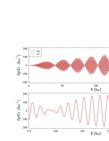
Figure 1: Density of states for the Hamiltonian (3) with $\epsilon=0.01$, Gaussian-averaged with a width $\gamma=0.5\hbar\omega$, versus energy $E$ (units: $\hbar\omega$). Dashed lines (red): quantum-mechanical results. Solid lines (black): semiclassical results using the uniform trace formula (71).

$$\delta g_{sc}(E)\simeq\sum_{po}{\cal A}_{po}(E)\,e^{-[\gamma T_{po}(E)/2\hbar]^{2}}\cos\,[S_{po}(E)/\hbar-\sigma_{po}\pi/2]\,,$$ (74)

so that orbits with longer periods $T_{po}$ will be exponentially suppressed.

In Fig. 1 we show a comparison of the results obtained with the uniform trace formula (71) for the case $\epsilon=0.01$ with those obtained from the exact numerical quantum spectrum. The width of the Gaussian smoothing was chosen to be $\gamma=0.5\hbar\omega$; in the semiclassical result the harmonics $k>2$ then do not contribute noticeably. The agreement is seen to be perfect; tiny differences can only be noted near the beat minima on the amplified scale below.

In Fig. 2 we show a similar comparison for $\gamma=0.1\hbar\omega$, exhibiting much fine structures. We now start to resolve the spectrum with a higher resolution; note that we still only plot the oscillating part $\delta g(E)$ of the density of states. In the top panel, the semiclassical result includes harmonics (i.e., repetitions of the two orbits) with $k\leq k_{m}=7$. This is evidently sufficient to reproduce the quantum-mechanical oscillations up to $E\simeq 45\hbar\omega$ with a high accuracy. In the centre panel, we have added two more harmonics, going up to $k\leq k_{m}=9$. Here we recognise the appearance of divergences at the scaled energies $e=0.361712$ and $e=0.437867$ which correspond to the bifurcations of the 19:9 and 17:8 tori from the repetitions of the circle orbit with $k=9$ and $k=8$, respectively (cf. Table 1 below). The small wiggles close to the divergences, with decreasing amplitudes when going away from them, are due to the missing contributions from those torus orbits in the trace formula (71) (see the following section).

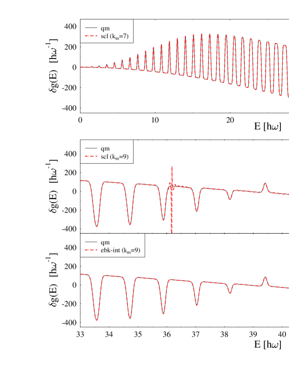
Figure 2: Same as Fig. 1, but with $\gamma=0.1\hbar\omega$. Top panel: including up to $k_{m}=7$ harmonics in the trace formula (71). Centre panel: adding harmonics up to $k_{m}=9$. Note the divergences due to the bifurcations of the 17:8 and 19:9 tori at the energies $E\simeq 43.79$ and $E\simeq 36.17$, respectively. Bottom panel: result obtained from the EBK trace integral (46), doing the integration over $l$ numerically, with $-k_{m}\leq M\leq+k_{m}$, $-2k_{m}\leq N\leq+2k_{m}$ using $k_{m}=9$.

In order to anticipate the results of a suitable uniform trace formula including the contributions of the tori, we show in the bottom panel of Fig. 2 the result of the EBK trace integral (46) obtained by a numerical integration over the variable $l$. Hereby the summations over $N$ and $M$ have been done in the limits $-k_{m}\leq M\leq+k_{m}$, $-2k_{m}\leq N\leq+2k_{m}$ using $k_{m}=9$. [The period to be used in the Gaussian damping factor of (74) is in this case given by $T_{po}=NT_{r}(e,L)$.] Now the divergences and all other discrepancies have disappeared; the difference to the quantum-mechanical result can hardly be recognised. The integral (46) therefore is also a uniform expression for the semiclassical density of states, containing the contributions of all periodic orbits. The numerical evaluation becomes, however, very time consuming for even finer energy resolutions (i.e., still smaller values of $\gamma$).

Our main result here is that up to a rather fine resolution, the shell structure of the present perturbed HO system is dominated by the two-fold degenerate families of diameter and circle orbits, although these are not the most degenerate orbits. This is a rather unusual situation, due to the fact that the shortest tori with the highest degeneracy are considerably longer (by a factor  $\sim$ $>$ 10) than the primitive diameter and circle orbits.

Let us finally test the range of validity of the perturbative trace formula (22). In Fig. 3 we compare its results to that of the full trace formula (71) for the two values $\epsilon=0.001$ (upper panel) and $\epsilon=0.01$ (lower panel). As expected, the two curves agree in the limit $e\to 0$. However, already for $\epsilon=0.001$ the amplitude modulation of the perturbative result deviates so much that the position of the first beat node is predicted by about 10% too low in energy. For $\epsilon=0.01$, the perturbative result becomes so bad that it predicts the second beat node approximately at the position of the correct first one. These results underline the fact that in yylund , the quantum results for weak interactions could be qualitatively reproduced by the perturbative trace formula, but not quantitatively with correct positions of the beat nodes. A more detailed analysis of the selfconsistent HF results of yylund using the uniform trace formula (71) is in progress magnus .

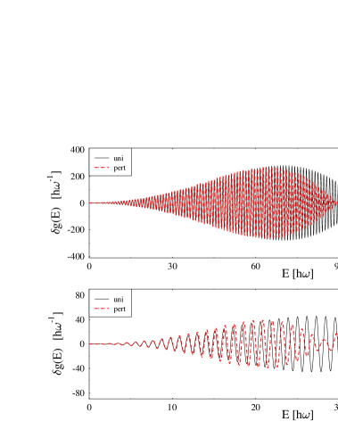
Figure 3: Same quantity as shown in Fig. 1. Here we compare the results of the perturbative trace formula (22) (dashed lines, red) and those of the uniform trace formula (71) (full lines, black), Gaussian-averaged with $\gamma=0.5\hbar\omega$. Upper panel: for $\epsilon=0.001$; lower panel: for $\epsilon=0.01$.

III.6 Bifurcations of rational tori from the circle orbit

As we have seen in the previous section, periodic orbit with both angular and radial motion appear as the rational tori fulfilling the periodicity condition (54). For the Hamiltonian (3), this condition can only be fulfilled in the limits given in (70). This means that stationary points $L_{N\!M}$ of the $L$ integral in (46) satisfying (50) and hence (54) only exist if $2<|N\!:\!M|<\sqrt{6}$. Hereby $|M|$ corresponds to the repetition number $k$ of the circle orbit that undergoes a bifurcation exactly when $L_{N\!M}$ is equal to the maximum angular momentum $L_{m}$. In Table 1 we list some of the lowest energies $e_{N:M}$ at which this happens for the smallest integers $M=k$. Each of the $N\!\!:\!\!M$ tori only exists above its bifurcation energy, i.e., at energies $e>e_{N:M}$.

$M=k$	$N$	$~{}~{}~{}e_{N:M}$	$~{}l_{N\!M}$	$l_{N\!M}^{(\epsilon=\infty)}$
…	…	…	…	…
9	19	0.3617121	0.3370	0.276
8	17	0.4378671	0.4032	0.316
7	15	0.5527726	0.5009	0.360
6	13	0.7441150	0.6584	0.420
5	11	1.1174198	0.9508	0.504
4	9	2.0966668	1.6553	0.633
3	7	7.6699999	4.9331	0.864

Table 1:   Bifurcation energies $e_{N:M}$ and angular momenta $l_{N\!M}$ of the rational $N\!\!:\!\!M$ tori at which the stationary conditions (50) and (54) are fulfilled for the lowest values of $M$ and $N$. In the last column we give the angular momenta $l_{N\!M}$ for the limiting case $\epsilon\to\infty$ in which they do not depend on the energy (cf. Sect. III.7).

The contributions of the bifurcated tori to the semiclassical trace formula is obtained by a stationary-phase evaluation of the $l$ integral in (46), leading to

$$\delta g_{tori}(e)=\sum_{N>2M>0}{\cal A}^{T}_{N\!M}(e)\,(-1)^{N\!+\!M}\!\cos\left(\frac{S^{T}_{N\!M}(e)}{\hbar}+\frac{\pi}{4}\right).$$ (75)

The summation goes only over those pairs $N,M$ of positive integers for which the stationary condition (54) can be fulfilled. (Note that the contribution of the corresponding pairs of negative integers is included in the amplitudes by a factor 2.) The actions of the tori are given by

$$S^{T}_{N\!M}(e)=NS_{r}(e,l_{N\!M})+M2\pi L_{N\!M}(e)\,,$$ (76)

and their amplitudes by

$${\cal A}^{T}_{N\!M}(e)=\frac{2\sqrt{2s}}{\sqrt{\pi}\hbar^{5/2}}\,T_{r}(e,l_{N\!M})L_{N\!M}(e)\left(\!N\left|\frac{\partial^{2}s_{r}(e,l)}{\partial l^{2}}\right|_{l=l_{N\!M}(e)}\right)^{\!\!-1/2}\theta(e-e_{N:M})\,,$$ (77)

where $s$ is the action unit given in (37). The Heaviside step function in (77) is defined as

$$\theta(x)=0\quad\hbox{for}\quad x<0\,,\qquad\theta(x)=1/2\quad\hbox{for}\quad x=0\,,\qquad\theta(x)=1\quad\hbox{for}\quad x>0\,,\qquad$$ (78)

where the value 1/2 for $x=0$ accounts for the fact that one obtains only half a Fresnel integral when the stationary point is the upper end point of the integral in (46). The power $\hbar^{-5/2}$ in the amplitude ${\cal A}_{N\!M}(e)$ is characteristic of the three-fold degenerate orbits in a three-dimensional spherical system struma ; crli1 .

Eq. (75) corresponds to the standard Berry-Tabor trace formula bertab for the most degenerate orbits in an integrable system. Here, however, each contribution to (75) is only valid if the energy $e$ is sufficiently larger than the corresponding bifurcation energy $e_{N:M}$. In the neighbourhood of the bifurcation energies, we have to replace the sum of the diverging circle orbit contribution and the corresponding torus contribution with $|M|=r$ by a common uniform contribution. As it is well-known from the semiclassical theory of bifurcations ozoha ; ssun , one has to include hereby also the contributions of so-called “ghost orbits”, which are the imaginary (or complex) continuations of the bifurcated orbits (here: the tori) to the other side of the bifurcation (here: $e<e_{N:M}$).

It is, however, not the purpose of our present paper to discuss in more detail the uniform approximation suitable for this situation. The present scenario is actually almost identical to that described in kaidel for the bifurcations of tori in the integrable Hénon-Heiles system. Although there the orbit from which the tori bifurcate is an isolated one, while it here is a family of circle orbits, the uniform trace formula given in kaidel can be applied to the present system in a straightforward manner. We refer the interested reader to this paper for all the detailed formulae as well as for a numerical demonstration showing how diverging discrepancies of the type seen in the centre part of Fig. 2 disappear when a proper uniform trace formula is used. Its result would here be practically indistinguishable from the result shown in the bottom part of Fig. 2, in which we have evaluated the integral in (46) numerically instead of using the stationary phase approximation with end-point corrections.

III.7 The limit of the purely quartic oscillator

In this section we discuss briefly a purely quartic oscillator potential, i.e., we start from the Hamiltonian

$$H({\bf r},{\bf p})=\frac{1}{2}\,p^{2}+\frac{\epsilon}{4}\,r^{4}=E\,.$$ (79)

Here both the energy and $\epsilon$ can be scaled away. After dividing the above equation by $E$ and introducing the scaled variables

$$q_{i}=\left(\!\frac{\,\epsilon}{E}\right)^{\!1/4}\!r_{i}\,,\qquad\tau=(\epsilon E)^{1/4}\,t\,,\qquad l=\epsilon^{1/4}E^{-3/4}L\,,$$ (80)

we obtain the “unit energy” equation

$$1=\frac{1}{2}\,{\dot{q}}^{2}+\frac{1}{4}\,q^{4}+\frac{l^{2}}{2q^{2}}\,,$$ (81)

where the dot again means derivative with respect to the scaled time $\tau$. Hence the classical equations of motion become independent of energy and $\epsilon$. After obtaining all the classical results, we can reintroduce $E$ and $\epsilon$ just by remembering that lengths scale with $(E/\epsilon)^{1/4}$, momenta with $\sqrt{E}$, times (periods) with $(E\epsilon)^{-1/4}$, actions and angular momenta with $\epsilon^{-1/4}E^{3/4}$.

We obtain the semiclassical trace formula from the results of the previous sections and of the appendix C simply by taking the limit $\epsilon\to\infty$, which means practically by extracting the leading terms for $e\to\infty$. In this way, we obtain the following primitive periods and actions for the circle orbit:

$$T_{c}(E)=2\pi\epsilon^{-1/4}(4E/3)^{-1/4}\,,\qquad S_{c}(E)=2\pi L_{m}(E)\;=\;2\pi\epsilon^{-1/4}(4E/3)^{3/4}\,,$$ (82)

and for the diameter orbit:

$$T_{d}(E)=2\sqrt{2}\,\epsilon^{-1/4}K_{0}E^{-1/4}\,,\qquad S_{d}(E)=2\sqrt{2}\,\epsilon^{-1/4}(4/3)K_{0}E^{3/4}\,.$$ (83)

Here $K_{0}$ is the constant elliptic integral

$$K_{0}=K(\kappa_{0})=1.8540746773\dots\,,\qquad\kappa_{0}=1/\sqrt{2}\,.$$ (84)

Furthermore we get

$$T_{r}(E,L_{m})=\pi(3\epsilon E)^{-1/4}\,.$$ (85)

The resonance condition (54) becomes independent of the energy

$$\frac{T_{\phi}(E,l_{N\!M})}{T_{r}(E,l_{N\!M})}=w(l_{N\!M})=\frac{N}{M}\,,$$ (86)

since both periods scale with the same power of the energy. For the frequency ratio we find the limits

$$2\leq w(l_{N\!M})=N\!:\!M<\sqrt{6}\qquad\hbox{for}\qquad 0\leq l_{N\!M}<l_{m}=(4/3)^{3/4}=1.240806\dots$$ (87)

Note that the upper limit $l_{m}$ never becomes a stationary point, so that no bifurcations of the circle orbits occur in this system. The values of the stationary points $0<l_{N\!M}<l_{m}$ (in scaled dimensionless units) for the lowest values of $N$ and $M$ are given in the rightmost column of Table 1; as we just have seen, they do not depend on the energy $E$.

The result $w(l_{m})=\sqrt{6}$ is a special case of the general result, given in arita , that for a potential $V(r)$ = $U_{0}\,r^{\beta}$ one has $w(l_{m})=\sqrt{\beta\!+\!2}$.

For the amplitudes of the circle and diameter orbits in the trace formula (71), which keeps the same form, we obtain here

$${\cal A}_{k}^{c}(E)=\frac{4}{\hbar^{2}\sqrt{3}}\,\sqrt{\!\frac{E}{\epsilon}}\,\frac{(-1)^{k}}{\sin(k\pi\sqrt{6})}\,,\qquad{\cal A}_{k}^{d}(E)=\frac{4K_{0}^{2}}{\hbar^{2}\pi^{2}}\,\sqrt{\!\frac{E}{\epsilon}}\;\frac{(-1)^{k+1}}{k}\,.$$ (88)

The actions $S_{c}$ and $S_{d}$ to be used in (71) are those given in (82) and (83). Finally, the TF level density is found to be

$$g_{TF}(E)=\frac{4\sqrt{2}\,E^{5/4}}{5K_{0}\hbar^{2}\epsilon^{3/4}}\,.$$ (89)

The tori, which in the perturbed HO system discussed in the last section occur only at sufficiently high energies after their bifurcations from the repeated circle orbits, exist in the present system at all energies. However, they affect again only the finer quantum structures of the density of states since they only exist for $N\!:\!M\geq 7\!:\!3$ due to the selection by their resonance condition (87) (cf. also Table 1). This is demonstrated in the following two figures.

In Fig. 4, we compare the results of the semiclassical trace formula (71) for the diameters and circles using the above quantities to the exact quantum-mechanical density of states, both Gaussian-averaged over a width $\gamma=0.5$ (in energy units). The agreement is again perfect even on the enlarged scale in the lower part of the figure. The reason is that for the chosen energy resolution with $\gamma=0.5$, only repetition numbers $|M|=k<3$ contribute, for which there exist no tori (see Table 1).

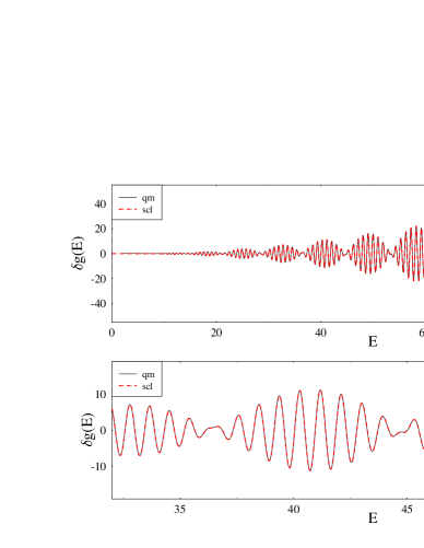
Figure 4: Density of states for the Hamiltonian (79) with $\epsilon=0.01$, Gaussian-averaged with a width $\gamma=0.5$ energy units. Dashed lines (red): quantum-mechanical results. Solid lines (black): semiclassical results using the uniform trace formula (71) and the actions and amplitudes given in (82), (83) and (88) with $k\leq 2$.

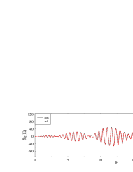
Figure 5: Same as Fig. 4, but with $\gamma=0.2$ energy units. Repetitions of the diameter and circle orbits with $k\leq 5$ are included in the semiclassical result.

Fig. 5 shows the same comparison for $\gamma=0.2$. Here some small discrepancies appear which become more visible with increasing energy. They are due to the missing contributions from the tori with $|M|=k\geq 3$. Since there are no bifurcations involved in the present system, the contributions of the tori are given by the Berry-Tabor trace formula (75), employing the appropriate expressions for the actions and periods used therein. The analytical expression of the action integral $S_{r}(e,l)$ in terms of elliptic integrals is the same as for the perturbed HO potential, as given in Eqs. (114) - (120), except that here the term $q^{2}\!/2$ in the potential and the corresponding contribution $s_{r}^{(1)}(e,l)$ must be omitted.

Even at the rather fine resolution obtained in Fig. 5, our main result is the observation that the circle and diameter orbits dominate the shell structure also for the purely quartic oscillator.

IV Summary and conclusions

Motivated by recent Hartree-Fock (HF) calculations of harmonically trapped fermionic gases with a repulsive interaction yylund , in which pronounced super-shell effects were obtained, we have developed a semiclassical trace formula for the density of states of the anharmonically perturbed three-dimensional isotropic harmonic oscillator (HO) defined in (3). We find that its gross-shell structure is dominated by the periodic orbits of diameter and circle shape, whose interference leads to super-shell beats which explain the findings from the numerical HF results.

In a first step, we have used the perturbative approach of Creagh crpert to describe the symmetry breaking U(3) $\to$ SO(3) for weak anharmonicities $\epsilon$, resulting in the perturbative trace formula (22). It uniformly restores the U(3) limit, yielding the exact trace formula (8) of the unperturbed HO system in the limit $\epsilon\to 0$. For the derivation of the perturbative result (22), one must in principle integrate over the 4-fold degenerate families of unperturbed HO orbits which cover the manifold $\mathbb{C}$P². As shown in App. B, however, it turns out to be easier to integrate over the energy shell in phase space, which is a five-sphere S⁵, whereby the integration can be reduced, under exploitation of the SO(3) symmetry, to the one-dimensional integral given analytically in (21). An interesting result hereby is the fact that its two contributions, corresponding to the diameter and circle orbits, already have the characteristic form occurring in the general trace formula (2). Usually, this form is obtained from a perturbative trace formula only asymptotically in the semiclassical limit $\hbar\to 0$; this happens, e.g., also when one investigates the corresponding Hamiltonian (3) in two dimensions or other perturbed 2-dimensional systems book ; crpert ; bcl .

Next we have used the standard EBK quantisation and the Poisson summation formula to derive a general semiclassical trace formula for arbitrary central potentials in terms of a one-dimensional integral over the angular momentum $L$ of the classical orbits, given in (46). Exact integration and summation over all $M,N$ yields, to leading order in $\hbar$, the EBK spectrum. Its asymptotic evaluation in the limit $\hbar\to 0$ yields the standard-type contributions to the trace formula (2). The end-point contributions yield the diameter orbits with $L=0$ and the circle orbits with maximum angular momentum; both contributions are of next-to-leading order in $\hbar$, whereas the leading-order contributions corresponding to the typical rational tori of integrable systems according to the Berry-Tabor theory bertab come from the stationary points inside the integration interval. One interesting mathematical aspect is the mechanism by which the ratio $\omega_{r}:\omega_{\phi}=2$ of radial to angular frequency of the diameter orbit is naturally selected by a property of the general radial action integral $S_{r}(E,L)=\oint p_{r}(E,L,r)\,dr$ as a function of angular momentum $L$ which appears to be universal for regular spherical potentials. It holds also for a particle in a spherical box with specular reflection, for which we have re-derived in Appendix D.1 the trace formula given by Balian and Bloch bablo from our general formula (46), taking into account the changes of the Maslov indices due to hard-wall reflections). The Coulomb potential, for which $\omega_{r}:\omega_{\phi}=1$, is discussed in Appendix D.2 where we also re-derive the exact trace formula for the Rydberg spectrum given in book .

For the Hamiltonian (3), we have derived a uniform trace formula for the diameter and circle orbit contributions that is valid for arbitrary $\epsilon$. We find that for low energies and low repetition numbers no tori exist, so that the gross-shell structure of this system is dominated by the circle and diameter orbits and their lowest repetitions. The tori bifurcate, at sufficiently high energy, out of the repetitions with $k\geq 3$ of the circle orbits, as was also observed recently for homogeneous power-law potentials in arita . Their contributions sufficiently high above the respective bifurcation energies are given by the usual Berry-Tabor type trace formula (75). We have not discussed here the common uniform treatment of the circle orbits and the tori bifurcating from them, since this scenario is identical to the one discussed in detail in kaidel . The same qualitative results are found also in the limit $\epsilon\to\infty$ in which the potential becomes a purely quartic oscillator. Although the tori with $N\!:\!M\geq 7\!:\!3$ here exist at all energies, they are so much longer (by a factor $\,\hbox{\kern 1.00006pt\lower 2.58334pt\hbox{$\sim$} \kern-11.19997pt\raise 2.58334pt\hbox{$>$} }10$) than the shortest diameter and circle orbits that they only affect the finer details of the quantum spectrum.

We thus have found the interesting and quite atypical situation of a three-dimensional system in which the periodic orbits with highest, i.e., three-fold degeneracy are only responsible for finer details of the quantum spectrum, whereas its gross-shell structure is to an astonishing degree dominated by the orbits of next-to-leading order in $\hbar$, i.e., the diameter and circle orbits occurring in two-fold degenerate families. This is totally different from the situation, observed first by Balian and Bloch bablo , of a spherical cavity potential (with ideally reflecting walls) which has turned out to be a realistic model for large spherical metal clusters. (We re-derive the semiclassical trace formula of Balian and Bloch for the spherical cavity in Appendix D.1.) There the famous super-shells nish ; klavs ; mbclus come from the interference of the shortest three-fold degenerate tori (the triangle and square orbits), whereas the two-fold degenerate diameter orbit family has virtually no effect on the observable shell structure of these systems.

Our results explain qualitatively the numerical quantum-mechanical HF results yylund for harmonically trapped fermionic atom gases. A more quantitative comparison, in which the strength $\epsilon$ of the perturbation in (3) is determined directly from the numerically obtained self-consistent HF potentials, is in progress magnus .

Lazzari et al. lazz have studied the periodic orbits in a spherical Woods-Saxon potential in connection with the physics of metal clusters and thereby focused on the contributions of the diameter orbits. We find agreement of their results for the tori and the diameters with our results (75), (77) and (64), respectively, if we interpret their function $\tau(L_{M},E)$ as being half the radial period $T_{r}(E,L_{N\!M})$ at the corresponding stationary value $L_{N\!M}$ of the angular momentum (= 0 for the diameters). They have, however, neglected the contributions from the circle orbits; furthermore they did not compare their semiclassical results with quantum-mechanical results. We suspect that the neglect of the circle orbits might be justifiable due to the chosen steepness of their Woods-Saxon potential, for which the triangle-like tori are perhaps more important than the circles.

Ozorio de Almeida et al. ozotom have discussed the summation of all periodic orbits in integrable systems in connection with spectral determinants. They conclude that edge corrections corresponding to lower-degenerate orbits may be neglected because they are implicitly approximated by the nearest-lying rational tori (characterised by very large numbers $M,N$ in our notation). While their argument applies to the full quantisation of the exact (or EBK-approximated) quantum spectrum obtained by summing over all orbits, it cannot be used when the spectrum is coarse-grained with a finite energy window $\gamma$, such as we have used the periodic-orbit sum in our present investigation (cf. also the discussion in the appendix of Ref. ozotom ) which is more practically oriented.

Appendix A Parametrisation the manifold $\mathbb{C}$P²

We reproduce here the parametrisation of $\mathbb{C}$P² given in bbz . We start with three complex numbers $Z_{\alpha}\in\mathbb{C}$:

$$(Z_{1},Z_{2},Z_{3})=(n_{1},n_{2}e^{i\nu_{2}},n_{3}e^{i\nu_{3}})\,,$$ (90)

with $n_{\alpha}\in\mathbb{R}$, $0\leq n_{\alpha}\leq 1\;(\alpha=1,2,3)$, and $\nu_{j}\in\mathbb{R}$, $0\leq\nu_{j}<2\pi\;(j=2,3)$, whereby the $n_{\alpha}$ are restricted to

$$n_{1}^{2}+n_{2}^{2}+n_{3}^{2}=1\,.$$ (91)

The $Z_{\alpha}$ define the complex projective space $\mathbb{C}$P². The $n_{\alpha}$ are in one-to-one correspondence with the points on the first octant of the 2-sphere $S^{2}$, and the $\nu_{j}$ form a 2-torus. At the edges of the octant, the torus contracts to a circle or to a point, and one or both of the $\nu_{j}$ are not defined.

Physically, we interpret the real and negative imaginary parts of the $Z_{\alpha}$ as coordinates and momenta, respectively, of a starting point $({\bf r}_{0},{\bf p}_{0})=(\{r_{\alpha}(0)\},\{p_{\alpha}(0)\})$

$$r_{\alpha}(0)=\Re e\,Z_{\alpha}\,,\qquad p_{\alpha}(0)=-\Im m\,Z_{\alpha}\,,$$ (92)

in the 6-dimensional phase space $({\bf r}(t),{\bf p}(t))=(\{r_{\alpha}(t)\},\{p_{\alpha}(t)\})$ of the 3-dimensional isotropic harmonic oscillator. The Hamiltonian (4), which has U(3) symmetry lipkin , is given by

$$H({\bf r},{\bf p})=\frac{1}{2}\sum_{\alpha=1}^{3}\left[\omega^{2}r_{\alpha}^{2}+p_{\alpha}^{2}\right]=E\,.$$ (93)

The $2\pi$-periodic solutions of the equations of motion are then given by

$$r_{\alpha}(t)=\Re e\,(Z_{\alpha}e^{i\omega t})\,,\qquad p_{\alpha}(t)=-\Im m\,(Z_{\alpha}e^{i\omega t})\,.$$ (94)

The equation (91) defines the energy shell, so that the six quantities $\{\omega r_{\alpha},p_{\alpha}\}$ are points on a 5-sphere, S⁵ (see also Appendix B below). By taking the total energy to be $E=1/2$ and setting $\omega=1$, we fix the radius of the 5-sphere to be unity. Taking out the phase factor $e^{i\omega t}$ takes us from S⁵ to the projective space $\mathbb{C}$P².

Using the Fubini-Study metric, the authors of bbz find the squared distance $ds^{2}$ between two points on $\mathbb{C}$P² to be

$$ds^{2}=dn_{1}^{2}+dn_{2}^{2}+dn_{3}^{2}+n_{2}^{2}(1-n_{2}^{2})\,d\nu_{2}^{2}+n_{3}^{2}(1-n_{3}^{2})\,d\nu_{3}^{2}-2\,n_{2}^{2}n_{3}^{2}\,d\nu_{2}d\nu_{3}\,.$$ (95)

The first three terms correspond to the standard metric on $S^{2}$, and the last three to the metric on a flat 2-torus whose shape depends on where we are on the octant.

We now wish to re-parametrise the $n_{\alpha}$ in terms of the two polar angles $(\vartheta,\varphi)$ on $S^{2}$ by writing

$$n_{1}=\cos\vartheta\,,\qquad n_{2}=\sin\vartheta\cos\varphi\,,\qquad n_{3}=\sin\vartheta\sin\varphi\,,$$ (96)

with $\vartheta,\varphi\in[0,\pi/2]$. Collecting our four angles in a vector $\psi$ by defining

$$\mbox{{\boldmath$\psi$ \unboldmath}}\!\!=(\psi_{1},\psi_{2},\psi_{3},\psi_{4})=(\vartheta,\varphi,\nu_{2},\nu_{3})\,,$$ (97)

we can write the squared distance $ds^{2}$ as

$$ds^{2}=\sum_{i,j=1}^{4}g_{ij}\,d\psi_{i}\,d\psi_{j}\,,$$ (98)

and find the elements $g_{ij}$ of the metric tensor to be $g_{11}=1$, $g_{22}=\sin^{2}\!\vartheta$, $g_{12}=g_{21}=0$, $g_{33}=\sin^{2}\!\vartheta\cos^{2}\!\varphi\,(1-\sin^{2}\!\vartheta\cos^{2}\!\varphi)$, $g_{44}=\sin^{2}\!\vartheta\sin^{2}\!\varphi\,(1-\sin^{2}\!\vartheta\sin^{2}\!\varphi)$, and $g_{34}=g_{43}=-\sin^{4}\!\vartheta\cos^{2}\!\varphi\sin^{2}\!\varphi$. From this, we get the integration measure on $\mathbb{C}$P² to be

$$d\Omega_{\mathbb{C}{\rm P}^{2}}=|{\rm det}(g_{ij})|^{1/2}d\psi_{1}d\psi_{2}\,d\psi_{3}\,d\psi_{4}=\sin^{3}\!\vartheta\cos\vartheta\,d\vartheta\,\cos\varphi\sin\varphi\,d\varphi\;d\nu_{2}d\nu_{3}\,.$$ (99)

The integrated volume of $\mathbb{C}$P², consistent with a general formula for $\mathbb{C}$Pⁿ, is

$$\Omega_{\mathbb{C}{\rm P}^{2}}=\int d\Omega_{\mathbb{C}{\rm P}^{2}}=\frac{\pi^{2}}{2\,}\quad\Leftarrow\quad\Omega_{\mathbb{C}{\rm P}^{n}}=\frac{\pi^{n}}{n!}\,.$$ (100)

Appendix B Integration of the modulation factor over S⁵

Here we give a strict proof of Eq. (21) of the modulation factor ${\cal M}$ for the anharmonically perturbed HO system (3). The most straightforward parametrisation of the six-dimensional phase space of the unperturbed HO is given in terms of the coordinate vector ${\bf r}(t)=\{r_{\alpha}(t)\}$ and the momentum vector ${\bf p}(t)=\{p_{\alpha}(t)\}$ $(\alpha=1,2,3)$. Since a periodic solution is uniquely determined by their initial values at $t=0$: ${\bf r}_{0}={\bf r}(0)$ and ${\bf p}_{0}={\bf p}(0)$, and the total energy $E=({\bf p}^{2}+\omega^{2}{\bf r}^{2})/2$ is a constant of motion, the six components of ${\bf r}_{0}$ and ${\bf p}_{0}/\omega$ must cover a 5-sphere with radius $R=\sqrt{2E}/\omega$. We introduce dimensionless coordinate and momentum vectors $\rho$ and $\pi$ , respectively, by

$$\mbox{{\boldmath$\rho$ \unboldmath}}\!\!=\frac{1}{R}\,{\bf r}_{0}\,,\qquad\mbox{{\boldmath$\pi$ \unboldmath}}\!\!=\frac{1}{R\omega}\,{\bf p}_{0}\,,$$ (101)

so that in these variables the energy shell becomes the unit sphere S⁵:

$$\mbox{{\boldmath$\rho$ \unboldmath}}\!\!^{2}+\mbox{{\boldmath$\pi$ \unboldmath}}\!\!^{2}=1\,.$$ (102)

From Eq. (18), the first-order action perturbation $\Delta S_{1}$ is given in terms of energy $E$ and angular momentum $L$ by

$$\Delta S_{1}=-\sigma\,(3-\omega^{2}L^{2}\!/E^{2})\,,$$ (103)

with $\sigma$ defined in (19). The modulation factor for the first-order perturbed HO system becomes therefore

$${\cal M}(k\sigma/\hbar)=\frac{1}{\pi^{3}}\!\int d\Omega_{S^{5}}\,e^{ik\Delta S_{1}\!/\hbar},$$ (104)

where $\Omega_{S^{5}}$ is the five-dimensional solid angle and $d\Omega_{S^{5}}$ is the integration measure on S⁵ with $\int d\Omega_{S^{5}}=\pi^{3}$. One may now express $\Delta S_{1}$ in (103) directly in terms of the five polar angles of six-dimensional hyperspherical coordinates, which becomes a very complicated function, and integrate (104) over all five angles. We have done this numerically and verified that it yields exactly the same result as the numerical 4-dimensional $\mathbb{C}$P² integration of (12) with the phase function (18).

It is, however, not necessary to perform the full five-dimensional integral for (104). We follow a much more economical route jaen , exploiting the rotational symmetry of the system and the SO(3) invariance of the expression (103) for $\Delta S_{1}$. Due to the restriction (102), we can write the S⁵ sphere as

$$S^{5}=\left\{(\cos\vartheta\,{\bf e}_{\rho},\sin\vartheta\,{\bf e}_{\pi})\Bigr{|}\;\vartheta\in[0,\pi/2]\,;\;{\bf e}_{\rho},{\bf e}_{\pi}\in S^{2}\right\},$$ (105)

where ${\bf e}_{\rho}$ and ${\bf e}_{\pi}$ are the unit vectors in the directions of $\rho$ and $\pi$ , respectively. The square of the conserved total angular momentum then is

$$L^{2}={\bf L}^{2}=({\bf r}_{0}\times{\bf p}_{0})^{2}=\frac{4E^{2}}{\omega^{2}}\cos^{2}\!\vartheta\,\sin^{2}\!\vartheta\,({\bf e}_{\rho}\times{\bf e}_{\pi})^{2}\,,$$ (106)

so that the action perturbation becomes, after the substitution $\alpha=2\vartheta$,

$$\Delta S_{1}=-\sigma[\,3-\sin^{2}\!\alpha\,({\bf e}_{\rho}\times{\bf e}_{\pi})^{2}]\,,\qquad\alpha\in[0,\pi].$$ (107)

The integration measure for (105) is

$$d\Omega_{S^{5}}=\cos^{2}\!\vartheta\,d\Omega_{S^{2}}({\bf e}_{\rho})\,\sin^{2}\!\vartheta\,d\Omega_{S^{2}}({\bf e}_{\pi})\,d\vartheta=\frac{1}{8}\sin^{2}\!\alpha\,d\alpha\,d\Omega_{S^{2}}({\bf e}_{\rho})\,d\Omega_{S^{2}}({\bf e}_{\pi})\,,$$ (108)

and the modulation factor becomes

$${\cal M}(k\sigma/\hbar)=\frac{1}{8\pi^{3}}\!\int_{0}^{\pi}d\alpha\,\sin^{2}\!\alpha\int d\Omega_{S^{2}}({\bf e}_{\rho})\int d\Omega_{S^{2}}({\bf e}_{\pi})\,e^{-ik\sigma[\,3-\sin^{2}\!\alpha\,({\bf e}_{\rho}\times{\bf e}_{\pi})^{2}]/\hbar}.$$ (109)

We now introduce the angle $\theta$ between the unit vectors ${\bf e}_{\rho}$ and ${\bf e}_{\pi}$, so that

$$({\bf e}_{\rho}\times{\bf e}_{\pi})^{2}=\sin^{2}\theta\,,$$ (110)

and choose ${\bf e}_{\rho}$ as the direction of the north pole ($\theta=0$) of polar angles $(\theta,\phi)$ for the vector ${\bf e}_{\pi}$. The integrand then becomes independent of ${\bf e}_{\rho}$, so that the corresponding S² integral just gives $\int\!d\Omega_{S^{2}}({\bf e}_{\rho})=4\pi$. For the other S² integral we have $\int\!d\Omega_{S^{2}}({\bf e}_{\pi})=2\pi\!\int_{0}^{\pi}\!\sin\theta\,d\theta$ since the integrand does not depend on $\phi$. We thus obtain, after the standard substitution $u=\cos\theta$ and an obvious reduction of the integration limits,

$${\cal M}(k\sigma/\hbar)=\frac{4}{\pi}\int_{0}^{\pi/2}d\alpha\,\sin^{2}\!\alpha\int_{0}^{1}du\,e^{-ik\sigma[\,3-\sin^{2}\!\alpha\,(1-u^{2})]/\hbar}.$$ (111)

Next, we make the substitution $t=u\sin\alpha$ and then a further substitution $s=\cos\alpha$ to obtain

$${\cal M}(k\sigma/\hbar)=\frac{4}{\pi}\int_{0}^{\pi/2}d\alpha\,\sin\alpha\int_{0}^{\sin\alpha}dt\,e^{-ik\sigma(3-\sin^{2}\!\alpha+t^{2})/\hbar}=\frac{4}{\pi}\int_{0}^{1}ds\int_{0}^{\sqrt{1-s^{2}}}dt\,e^{-ik\sigma(2+s^{2}+t^{2})/\hbar}.$$ (112)

Since the last integral goes exactly over the first quadrant of a unit disk in the $(s,t)$ plane, we can use polar coordinates $(r,\varphi)$ and furthermore $r^{2}=1-z$ to obtain our final result

$${\cal M}(k\sigma/\hbar)=\frac{4}{\pi}\int_{0}^{\pi/2}d\varphi\int_{0}^{1}dr\,r\,e^{-ik\sigma(2+r^{2})/\hbar}=\int_{0}^{1}dz\,e^{-ik\sigma(3-z)/\hbar},$$ (113)

which is identical to that given in (21) or in (56).

Appendix C Explicit integrals for the anharmonically perturbed HO

In this appendix we derive analytical expressions for the particular scaled potential $v(q)$ in (36). Rewriting the radial action integral (43) using the substitution $q^{2}=z$, we obtain

$$s_{r}(e,l)=2\int_{q_{1}}^{q_{2}}\!dq\sqrt{2e-q^{2}-q^{4}/2-l^{2}\!/q^{2}}=\frac{1}{\sqrt{2}}\int_{z_{1}}^{z_{2}}\frac{dz}{z}\sqrt{g(z)}\,,$$ (114)

where

$$g(z)=4ez-2z^{2}-z^{3}-2l^{2}=(z_{1}-z)(z_{2}-z)(z_{3}-z)\,.$$ (115)

The classical turning points are defined by the roots of the cubic equation $g(z)=0$, which are always real: the discriminant can easily be shown to be negative except for $l=l_{m}(e)$ where it becomes zero due to the double root $z_{1}=z_{2}$. Selecting the roots such that

$$z_{3}<z_{1}\leq z_{2}\,,$$ (116)

one finds that $z_{3}$ is always negative, whereas $z_{1}$ and $z_{2}$ are positive definite and represent the squares of the real classical turning points $q_{1}$ and $q_{2}$.

The integrals in (114) cannot be found in most tables. However, after an integration by parts we may write the r.h.s. as

$$s_{r}(e,l)=s_{r}^{(1)}(e,l)+s_{r}^{(2)}(e,l)-l^{2}s_{r}^{(-1)}(e,l)\,,$$ (117)

where we have defined

$$s_{r}^{(n)}(e,l)=\sqrt{2}\int_{z_{1}}^{z_{2}}dz\frac{z^{n}}{\sqrt{g(z)}}\,.$$ (118)

In Byrd and Friedman byfr , these integrals are found to be:

$$s_{r}^{(1)}(e,l) = \frac{2\sqrt{2}}{\sqrt{z_{2}-z_{3}}}\frac{z_{2}}{\kappa^{2}}\,[(\kappa^{2}-\alpha^{2})\,K(\kappa)+\alpha^{2}E\,(\kappa)]\,,$$

$$s_{r}^{(2)}(e,l) = \frac{2\sqrt{2}}{\sqrt{z_{2}-z_{3}}}\frac{z_{2}^{2}}{3\kappa^{4}}\,[(3\kappa^{4}-6\alpha^{2}\kappa^{2}+2\alpha^{4}+\kappa^{2}\alpha^{4})\,K(\kappa)+2\alpha^{2}(3\kappa^{2}-\alpha^{2}-\kappa^{2}\alpha^{2})\,E(\kappa)]\,,$$

$$s_{r}^{(-1)}(e,l) = \frac{2\sqrt{2}}{\sqrt{z_{2}-z_{3}}}\frac{1}{z_{2}}\,\Pi(\alpha^{2},\kappa)\,.$$ (119)

Here $K(\kappa)$, $E(\kappa)$ and $\Pi(\alpha^{2},\kappa)$ are the complete elliptic integrals of first, second and third kind with modulus $\kappa$, and

$$\kappa=\sqrt{\frac{z_{2}-z_{1}}{z_{2}-z_{3}}}\,,\qquad\alpha^{2}=1-\frac{z_{1}}{z_{2}}\,.$$ (120)

Note that $0\leq\kappa^{2}\leq\alpha^{2}\leq 1$, which corresponds to the ’circular case’ of the elliptic integral $\Pi(\alpha^{2},\kappa)$ byfr . This function becomes singular like $(1-\alpha^{2})^{-1/2}$, i.e., for $\alpha\to 1$ which happens when $l\to 0$. Since $z_{1}$ goes to zero like $l^{2}\!/2e$ in this limit, $\Pi(\alpha^{2},\kappa)$ has a first-order pole at $l=0$. Using the Laurent expansion of $\Pi(\alpha^{2},\kappa)$ given in Eq. 906.04 of byfr , we find

$$s_{r}^{(-1)}(e,l)=\frac{\sqrt{2}\pi}{\sqrt{-z_{1}z_{2}z_{3}}}-2a(e)+{\cal O}(l)=\frac{\pi}{l}-2a(e)+{\cal O}(l)\,,$$ (121)

with

$$a(e)=-\frac{\sqrt{2}}{z_{2}^{0}\sqrt{z_{2}^{0}-z_{3}^{0}}}\left[K(\kappa_{0})-\frac{E(\kappa_{0})}{(1-\kappa_{0}^{2})}\right]=\frac{\pi}{8}\left(1-\frac{15}{8}\,e+\dots\right).$$ (122)

Here $z_{i}^{0}$ and $\kappa_{0}$ are the $l=0$ values of the quantities given in Eqs. (127) and (128) below. The last equality in (121) follows because $z_{1}z_{2}z_{3}=-2l^{2}$, as seen from (115). The functions $s_{r}^{(n)}(e,l)$ with $n=1,2$ are both regular in $l=0$. Altogether we obtain the following Taylor expansion for the total radial action integral (117):

$$s_{r}(e,l)=s_{r}(e,0)-\pi\,l+a(e)\,l^{2}+{\cal O}(l^{3})\,,$$ (123)

The radial period (44) is easily found to be

$$t_{r}(e,l)=s_{r}^{(0)}(e,l)=\frac{\;2\sqrt{2}}{\sqrt{z_{2}-z_{3}}}\,K(\kappa)\,.$$ (124)

In the limit $l=0$, which is relevant for the diameter orbits and the TF density of states, the above results simplify considerably. We obtain

$$s_{r}(e,0) = \frac{2}{3}\,(1+4e)^{1/4}\left[\left(\sqrt{(1+4e)}+1\right)K(\kappa_{0})-2E(\kappa_{0})\right],$$ (125)

$$t_{r}(e,0) = 2\,(1+4e)^{-1/4}K(\kappa_{0})\,.$$ (126)

Note that in this limit we get

$$z_{1}^{0}=0\,,\qquad z_{2}^{0}=(q_{2}^{0})^{2}=\sqrt{1+4e}-1\,,\qquad z_{3}^{0}=-\sqrt{1+4e}-1\,,$$ (127)

and the modulus of the elliptic integrals becomes

$$\kappa_{0}=\sqrt{\frac{z_{2}^{0}-z_{1}^{0}}{z_{2}^{0}-z_{3}^{0}}}=\sqrt{\frac{\sqrt{1+4e}-1}{2\sqrt{1+4e}}}=\sqrt{e}\left(1-\frac{3}{2}\,e+\dots\right).$$ (128)

The TF expression (48) for the density of states becomes

$$g_{TF}(e) = \frac{8}{15\pi\hbar^{3}}\,\frac{\omega^{5}}{\epsilon^{2}}\,(1+4e)^{1/4}\,[2(1+3e)E(\kappa_{0})-(1+3e+\sqrt{1+4e})K(\kappa_{0})]\,.$$ (129)

It is of interest to see the first terms in the Taylor expansion of the above results around $e=0$, whose leading terms are those of the pure harmonic oscillator:

$$s_{r}(e,l) = \pi\,(e-l)-\frac{1}{8}\,\pi\,(3e^{2}-l^{2})+\dots\,,$$ (130)

$$t_{r}(e,l) = \pi-\frac{3}{4}\,\pi\,e+\frac{15}{64}\,\pi(7e^{2}-l^{2})+\dots\,,$$ (131)

$$g_{TF}(e) = \frac{1}{2\hbar^{3}}\,\frac{\omega^{5}}{\epsilon^{2}}\,e^{2}(1-5e/4+\dots)\,.$$ (132)

The unscaled leading HO terms are

$$S_{r}^{ho}(E,L)=\pi\!\left(\frac{E}{\omega}-L\right)=\pi[L_{m}(E)-L]\,,\qquad T_{r}^{ho}=\frac{\pi}{\omega}\,,\qquad g_{TF}^{ho}(E)=\frac{E^{2}}{2(\hbar\omega)^{3}}\,.$$ (133)

The diameter orbit with $L=0$ makes two full radial oscillations during its primitive period. Therefore its primitive action and period are given by

$$S_{d}(e)=2S_{r}(e,0)\,,\qquad T_{d}(e)=2T_{r}(e,0)\,.$$ (134)

For the circle orbit, the primitive action integral $S_{c}(e)$ is just $2\pi$ times the maximum value of the angular momentum, $L_{m}(e)=s\,l_{m}(e)$, which for the present potential is found to be

$$L_{m}(e)=s\sqrt{\frac{8}{27}\,[(1+3e)^{3/2}-1-9e/2]}\,,\qquad S_{c}(e)=2\pi L_{m}(e)=\frac{2\pi E}{\omega}\,(1-e/4+\dots)\,.$$ (135)

The primitive period of the circle orbit is given by its energy derivative

$$T_{c}(e)=\pi\frac{\sqrt{6}}{\omega}\,\frac{(1+3e)^{1/2}-1}{\sqrt{(1+3e)^{3/2}-1-9e/2}}=\frac{2\pi}{\omega}\,(1-e/2+\dots)\,.$$ (136)

We also give here the value of the radial period $T_{r}(e,l)$ at $l=l_{m}(e)$. The corresponding frequency $\omega_{r}(e,l_{m})=2\pi/T_{r}(e,l_{m})$ is easily obtained from the second derivative of the effective potential at its minimum $q_{0}$, which for the present potential is given by

$$q_{0}^{2}=z_{0}=2(\sqrt{1+3e}-1)/3\,,$$ (137)

using $\omega_{r}^{2}(e,l_{m})=V^{\prime\prime}_{eff}(q_{0})$, and the result becomes

$$T_{r}(e,l_{m})=\frac{2\pi}{\omega_{r}(e,l_{m})}=\frac{\pi}{\omega}\,(1+3e)^{-1/4}=\frac{\pi}{\omega}\,(1-3e/4+\dots)\,.$$ (138)

This agrees with the result obtained from (124), noting that for the maximum value of $l=l_{m}(e)$, $z_{1}=z_{2}=z_{0}$ and $z_{3}=-2(2\sqrt{1+3e}+1)/3$, so that $\kappa$ (120) becomes zero and $K(0)=\pi/2$.

Appendix D Trace formulae for other spherical potentials

In order to illustrate the validity and the usage of our general EBK trace integral (46), we present in this appendix briefly its application to two popular spherical potentials.

D.1 The spherical box potential

We consider a particle with mass $m=1$ in a spherical box with radius $R$ and ideal specular reflection from the boundary, i.e., a three-dimensional spherical billiard. Quantum-mechanically, one obtains the spectrum by solving the Schrödinger equation with Dirichlet boundary conditions. The semiclassical trace formula for this system has been derived by Balian and Bloch bablo using a multi-reflection expansion of the Green function. To derive it from our formula (46), we need the radial action integral for arbitrary energy $E\geq 0$ and angular momentum $0\leq L\leq L_{m}=R\sqrt{2E}$. Working throughout with unscaled variables, we find (with $r_{1}=L/\sqrt{2E}$)

$$S_{r}(E,L)=2\int_{r_{1}}^{R}dr\sqrt{2E-L^{2}\!/r^{2}} = 2\sqrt{2ER^{2}-L^{2}}-2L\arccos\,(L/R\sqrt{2E})$$ (139)

$$= 2R\sqrt{2E}-\pi L+L^{2}\!/R\sqrt{2E}+{\cal O}(L^{3})\,,$$

thus fulfilling our general relation (123) with

$$a(e)=1/R\sqrt{2E}\,.$$ (140)

With this, the stationary condition (54) gives

$$2N\arccos\,(L/R\sqrt{2E})=2\pi M$$ (141)

with the solutions

$$L_{N\!M}=R\sqrt{2E}\cos(\pi M/N).$$ (142)

As in the potentials discussed in Sect. III, the solution with $L=0$ corresponding to N=2M contributes only via the end-point correction of (46) to the diameter orbit with the primitive action

$$S_{d}(E)=2S_{r}(E,0)=4R\sqrt{2E}$$ (143)

and, according to the lower equation in (72), with the amplitude of its $k$-th repetition

$${\cal A}_{k}^{d}(E)=\frac{R^{2}}{\pi\hbar^{2}}\frac{1}{k}\,.\qquad(k=|M|)$$ (144)

The upper end-point correction with $L_{N\!M}=L_{m}=R\sqrt{2E}$ can, for $M\neq 0$, only be reached formally in the limit $N\to\infty$. It corresponds to the “whispering gallery mode” with amplitude ${\cal A}\propto 1/\sqrt{N}$, cf. (146) below, and does therefore not contribute to the trace formula. The tori with $0<L_{N\!M}<L_{m}$ have the actions

$$S^{T}_{N\!M}(E)=NS_{r}(E,L_{N\!M})+2\pi ML_{N\!M}=2NR\sqrt{2E}\sin\varphi_{N\!M}\,,\qquad\varphi_{N\!M}=\pi M/N\,.$$ (145)

This corresponds exactly to the actions of the polygonal orbits given in bablo with winding number $k=|M|\geq 1$ and $v=|N|>2k$ corners (i.e., reflections from the boundary). The case $v=2k$ corresponds to the $k$-th repetition of the diameter orbit. For the polygons, $\varphi_{vk}=\pi k/v$ is half the polar angle covered by one of their segments. The amplitudes of the tori with $v>2k$ become, according to (77),

$${\cal A}^{T}_{vk}(E)=\frac{2R^{5/2}(2E)^{1/4}}{\hbar^{5/2}\sqrt{\pi}}\sin(2\varphi_{vk})\sqrt{\frac{\sin\varphi_{vk}}{v}}\,.$$ (146)

Before we can write down the trace formula with the correct phases, we have to correct the radial quantisation condition (27), because the Maslov index changes from 1/4 to 1/2 per turning point if a reflection happens there. Hence the quantisation condition is $S_{r}=2\pi\hbar(n_{r}+1)$ for the diameter orbit and $S_{r}=2\pi\hbar(n_{r}+3/4)$ for the tori. This changes the phases in (46) and all the results derived from it. Taking this into account, we obtain the semiclassical trace formula for the spherical billiard

$$\delta g(E)=\sum_{v>2k>0}\!\!{\cal A}^{T}_{vk}(E)\,\sin[S^{T}_{vk}(E)/\hbar\!-\!3v\pi\!/2\!-\!k\pi+3\pi\!/4]-\sum_{k>0}{\cal A}_{k}^{d}(E)\,\sin[kS_{d}(E)/\hbar]\,,$$ (147)

which is identically the result of Balian and Bloch bablo .

D.2 The Coulomb potential

Here we derive the trace formula for the Coulomb potential as a special central potential which is not regular in $r=0$:

$$V(r)=-\frac{\alpha}{r}\,.$$ (148)

We need not use scaled variables here, but it is useful to introduce the positive energy $e=-E$ since all bound states in the potential (148) have $E<0$. The maximum angular momentum and the action of the circle orbit are

$$L_{m}(e)=\frac{\alpha}{\sqrt{2e}}\,,\qquad S_{c}(e)=\frac{2\pi\alpha}{\sqrt{2e}}\,,$$ (149)

from which the period of the circle orbit is found to be

$$T_{c}(e)=2\pi\frac{dL_{m}(e)}{dE}=\frac{\pi\alpha}{\sqrt{2}\,e^{3/2}}\,.$$ (150)

The radial action integral becomes elementary (cf. book ; ajp ):

$$S_{r}(e,L)=\sqrt{2}\int_{r_{1}}^{r_{2}}dr\sqrt{-e+\alpha/r-L^{2}\!/2r^{2}}=2\pi\!\left(\frac{\alpha}{\sqrt{2e}}-L\right)=2\pi[L_{m}(e)-L]\,.$$ (151)

From it we find the radial period

$$T_{r}(e)=\frac{\pi\alpha}{\sqrt{2}\,e^{3/2}}\,.$$ (152)

The difference from the other potentials treated in this paper is that the term linear in $L$ in (151) here has the coefficient $-2\pi$. Furthermore, we find from the general relation (52)

$$\frac{\partial S_{r}(e,L)}{\partial L}=-2\pi\qquad\Rightarrow\qquad\omega_{\phi}(e)=\omega_{r}(e)\,,\qquad T_{r}(e)=T_{\phi}(e)\,.$$ (153)

Thus, the radial and angular frequencies are identically the same for all values of the angular momentum $L$. This is a special property of Kepler’s ellipses. [Note that here, in contrast to the spherical HO, the angular momentum $L$ is defined with respect to one of the focal points and not to the symmetry centre of the ellipse!]

Inserting the above results into the general EBK trace integral (46) for the density of states, we obtain

$$g_{coul}(e)=\frac{T_{r}(e)}{\pi\hbar^{3}}\!\sum_{M,N=-\infty}^{\infty}\!(-1)^{M+N}\int_{0}^{L_{m}(e)}\!LdL\,e^{i2\pi[N(L_{m}-L)+ML]/\hbar}.$$ (154)

Due to (153), the general resonance condition (54) implies $N=M$ for all periodic orbits. We therefore only use the terms with $N=M=\pm k$ in the double sum of (154) (cf. the discussion at the end of Sect. III.3). We then find

$$g_{coul}(e)=\frac{\alpha^{3}}{\hbar^{3}(2e)^{5/2}}\left[1+2\sum_{k=1}^{\infty}\cos\left(\frac{k}{\hbar}\frac{2\pi\alpha}{\sqrt{2e}}\right)\!\right].$$ (155)

Writing this in terms of atomic units (note that we have put $m=1$)

$$E_{at}=\frac{\alpha^{2}}{2\hbar^{2}}=Ry\,,$$ (156)

we finally obtain the quantum-mechanically exact trace formula

$$g_{coul}(E)=\sum_{n=1}^{\infty}n^{2}\delta(E+E_{at}/n^{2})=\frac{E_{at}^{3/2}}{2(-E)^{5/2}}\left[1+2\sum_{k=1}^{\infty}\cos\left(2\pi k\sqrt{-E_{at}/E}\right)\!\right]\!,$$ (157)

which has been given in book . The eigenenergies

$$E_{n}=-\frac{E_{at}}{n^{2}}\,,\qquad\qquad(n=n_{r}+\ell+1)$$ (158)

with degeneracies $d_{n}=n^{2}$ are, as is well known, also found directly from the EBK quantisation conditions (27) - (29) using (151) and (31).

References

- (1) M. C. Gutzwiller, J. Math. Phys. 12, 343 (1971), and earlier papers quoted therein.
- (2) R. Balian and C. Bloch, Ann. Phys. (N.Y.) 69, 76 (1972).
-
(3)
V. M. Strutinsky, Nukleonika (Poland) 20, 679 (1975);
V. M. Strutinsky and A. G. Magner, Sov. J. Part. Nucl. 7, 138 (1976) [Elem. Part. & Nucl. (Atomizdat, Moscow) 7, 356 (1976)]. - (4) S. C. Creagh and R. G. Littlejohn, Phys. Rev. A 44, 836 (1991); S. C. Creagh, J. Phys. A 26, 95 (1993).
- (5) S. C. Creagh and R. G. Littlejohn, J. Phys. A 25, 1643 (1992).
- (6) M. Brack and R. K. Bhaduri: Semiclassical Physics (revised edition, Westview Press, Boulder, USA, 2003).
-
(7)
M. C. Gutzwiller: Chaos in Classical and Quantum
Mechanics (Springer Verlag, New York, 1990);
H.-J. Stöckmann: Quantum Chaos: an Introduction (Cambridge University Press, Cambridge, UK, 1999);
F. Haake: Quantum Signatures of Chaos (Springer, 2nd edition, 2001). - (8) M. V. Berry and M. Tabor, Proc. R. Soc. Lond. A 349, 101 (1976).
-
(9)
A. Einstein, Verh. Dtsch. Phys. Ges. 19, 82 (1917);
L. Brillouin, J. Phys. Radium 7, 353 (1926);
J. B. Keller, Ann. Phys. (N. Y.) 4, 180 (1958). - (10) Aa. Bohr and B. R. Mottelson: Nuclear Structure Vol. I (World Scientific, New York, 1975).
- (11) H. Nishioka, K. Hansen, and B. R. Mottelson, Phys. Rev. B 42, 9377 (1990).
- (12) J. Pedersen, S. Bjørnholm, J. Borggren, K. Hansen, T. P. Martin, and H. D. Rasmussen, Nature 353, 733 (1991).
- (13) M. Brack, Rev. Mod. Phys. 65, 677 (1993); The Scientific American, December 1997, p. 50.
- (14) S. M. Reimann and M. Manninen, Rev. Mod. Phys. 74, 1283 (2002).
- (15) A. I. Yanson, I. K. Yanson, and J. M. van Ruitenbeek, Nature 400, 144 (1999); Phys. Rev. Lett. 84, 5832 (2000).
- (16) A. M. Ozorio de Almeida and J. H. Hannay, J. Phys. A 20, 5873 (1987).
- (17) S. Tomsovic, M. Grinberg, and D. Ullmo, Phys. Rev. Lett. 75, 4346 (1995).
- (18) M. Brack, P. Meier, and K. Tanaka, J. Phys. A 32, 331 (1999).
-
(19)
M. Sieber, J. Phys. A 29, 4715 (1996);
H. Schomerus and M. Sieber, J. Phys. A 30, 4537 (1997);
M. Sieber and H. Schomerus, J. Phys. A 31, 165 (1998). - (20) see, e.g., H. J. Lipkin: Lie Groups for Pedestrians (North-Holland, Amsterdam, 1965).
- (21) Y. Yu, M. Ögren, S. Åberg, S. M. Reimann, and M. Brack, preprint arXiv:cond-mat/0502096 (2005).
- (22) S. C. Creagh, Ann. Phys. (N. Y.) 248, 60 (1996).
- (23) I. Bengtsson, J. Brännlund, and K. Życzkowski, Int. J. Mod. Phys. A 17, 4675 (2002).
- (24) see also L. J. Curtis and D. G. Ellis, Am. J. Phys. 72, 1521 (2004), for a pedagogical and concise presentation of EBK quantisation of spherical systems.
- (25) see, e.g., E. C. Titchmarsh: Introduction to the theory of Fourier Integrals (Second edition, Clarendon Press, Oxford, 1948), p. 60.
- (26) R. Wong: Asymptotic Approximation of Integrals (Academic Press Inc., San Diego, 1989).
- (27) M. V. Berry and K. E. Mount, Rep. Prog. Phys. 35, 315 (1972).
- (28) M. Abramowitz and I. A. Stegun: Handbook of Mathematical Functions, 9th printing (Dover, New York, 1970)
- (29) For stable orbits, see also W. H. Miller, J. Chem. Phys. 63, 996 (1975).
- (30) M. Ögren, work in progress.
- (31) J. Kaidel and M. Brack, Phys. Rev. E 70, 016206 (2004).
- (32) K. Arita, Int. J. Mod. Phys. E 13, 191 (2004).
- (33) M. Brack, S. C. Creagh, and J. Law, Phys. Rev. A 57, 788 (1998).
- (34) G. Lazzari, H. Nishioka, E. Vigezzi, and R. Broglia, Phys. Rev. B 53, 1064 (1996).
- (35) A. M. Ozorio de Almeida, C. H. Lewenkopf, and S. Tomsovic, J. Phys. A 35, 10629 (2002).
- (36) K. Jänich, private communication (2005).
- (37) P. F. Byrd and M. D. Friedman: Handbook of Elliptic Integrals for Engineers and Scientists (Springer-Verlag, Berlin, 2nd revised edition, 1971).