Ref. SISSA 35/2005/FM

On a Camassa-Holm type equation
with two dependent variables

Gregorio Falqui
SISSA, Via Beirut 2/4, I-34014 Trieste, Italy

Abstract: We consider a generalization of the Camassa Holm (CH) equation with two dependent variables, called CH2, introduced in [16]. We briefly provide an alternative derivation of it based on the theory of Hamiltonian structures on (the dual of) a Lie Algebra. The Lie Algebra here involved is the same algebra underlying the NLS hierarchy. We study the structural properties of the CH2 hierarchy within the bihamiltonian theory of integrable PDEs, and provide its Lax representation. Then we explicitly discuss how to construct classes of solutions, both of peakon and of algebro-geometrical type. We finally sketch the construction of a class of singular solutions, defined by setting to zero one of the two dependent variables.

1 Introduction

The relevance of Camassa Holm equation, first discovered by means of geometric considerations by Fokas and Fuchssteiner [11], was brought to the light in [6], where it was obtained as a suitable limit of the Green-Naghvi equations. One of its more interesting features is that it is an integrable approximation of an order higher than KdV to the Euler equations in one spatial dimension.

From the mathematical point of view, until quite recently the CH hierarchy was possibly the only well known example of integrable hierarchy not comprised in the Dubrovin-Zhang classification scheme of evolutionary bihamiltonian hierarchies [9]. The reason for this is that the CH hierarchy does not admit a formulation by means of a $\tau$-function. This lacking is reflected in the properties of notable classes of solutions. Indeed, bounded traveling waves for the CH equation (termed peakons) develop a discontinuity in the first derivatives, and the evolution properties of finite gap solutions, as discussed in [4, 17, 5], are somewhat peculiar, even if they can be expressed in terms of hyperelliptic curves as in the KdV case. The Whitham modulation theory associated with genus one solutions of CH, discussed in [1], also presents some non standard features.

The integrable equations we are going to discuss in the present paper are conservation laws for two dependent variables of the form:

$$\begin{array}[]{lcl}{(v-v_{x})_{t}}&=&(-2\rho u+v^{2}-vv_{x})_{x}\\ {(u+u_{x})_{t}}&=&(2uv+u_{x}v)_{x},\end{array}$$ (1.1)

with $\rho$ a parameter. These equations was derived (for $\rho=1$) in [16] within the framework of the general deformation theory of hydrodynamic hierarchies of bihamiltonian evolutionary PDEs [9]; more recently, a related equation has been considered in [7], within the framework of reciprocal transformations, and the properties of solitary waves and 2-particle like solutions described.

Actually, a similar equation was introduced by Olver and Rosenau in [18], as a deformation of the Boussinesq system; traveling wave solutions of the resulting equation can be found in [15]. In particular, in the paper [18], various non-standard integrable equations were defined. The key observation was that one can define bihamiltonian pencils from a given Poisson tensor using scaling arguments, and hence apply a recipe used in [11].

Our derivation of the equation resembles the one of [18]; however, on the one hand we will take advantage of the fact that the phase space is the dual of a Lie algebra, and, on the other hand, we will require that the hydrodynamical limit of the resulting equations be “substantially” the same as that of the classical equation we are starting from. As it will be briefly sketched in Section 3, the latter are the well known AKNS equations, that is, a complex form of the Nonlinear Schrödinger equations.

In the core of the paper we will study both formal and concrete properties of the hierarchy (1.1), which we call CH2 hierarchy. At first we will characterize it from the bihamiltonian point of view, find its Lax representation, and discuss the associated negative hierarchy.

Then we will discuss the features of two main classes of solutions. We will show that it admits peaked traveling waves, and show that these solutions can be consistently superposed, giving rise to the same finite dimensional Hamiltonian system associated with the N-peakon solution of the CH equation. Then we will address the problem of characterizing algebro-geometric solutions. We will show that the same phenomenon that happens in the Harry-Dym and CH finite gap solutions, namely the occurrence of non-standard Abel-Jacobi maps, is reproduced here.

We will end noticing that the reduction of the CH2 equations on the submanifold $u(x,t)=0$, where they yield the one-field equation

$$(v-v_{x})_{t}=(v^{2}-vv_{x})_{x}$$

admits weak solutions of traveling wave type with peculiar interaction properties.

2 Some remarks on the CH hierarchy

We herewith collect some remarks on the CH equation

$$u_{t}-u_{xxt}=-3uu_{x}+2u_{x}u_{xx}+uu_{xxx},$$ (2.1)

and highlight those features that will lead us to define its $2$-field generalization the next Sections. In particular, we will focus on a connection of CH with the KdV equation $u_{t}=-u_{xxx}+6uu_{x}$ which was (although implicitly) pointed out [14] in the framework of Euler equations on diffeomorphisms groups.

From the bihamiltonian point of view, the KdV theory can be regarded as the Gel’fand–Zakharevich [12] theory of the Poisson pencil

$$Q-\lambda P=-{\partial}_{x}^{3}+2u{\partial}_{x}+u_{x}-\lambda{\partial}_{x}.$$ (2.2)

defined on a suitable space ${\cal U}$ of functions $u=u(x)$ of one independent variable. As it has been long known, ${\cal U}$ admits a very natural geometrical interpretation of dual of the Witt algebra ${\cal V}$ of vector fields in “one dimension”, whose elements will be represented with $f\displaystyle{\displaystyle{\frac{\partial}{\partial x}}}$, endowed with the natural Lie bracket. Actually, a closer look at the expression of the KdV Poisson pencil 2.2 shows that, calling

$$Q_{\omega}={\partial}^{3}_{x},\quad P={\partial}_{x},\quad Q_{h}=2u{\partial}_{x}+u_{x},$$ (2.3)

we are facing a triple of Poisson tensors, $P,Q_{\omega},Q_{h}$, all of which have a well defined geometrical and algebraic meaning. Namely:

1. $Q_{h}$ is the Lie Poisson structure on ${\cal V}^{*}$.

2. $P$ is associated with the coboundary ${c}(f{\displaystyle{\frac{\partial}{\partial x}}},g{\displaystyle{\frac{\partial}{\partial x}}})=\oint fg_{x}$.

3. $Q_{\omega}$ is associated with the Gel’fand-Fuchs cocycle $\omega(f{\displaystyle{\frac{\partial}{\partial x}}},g{\displaystyle{\frac{\partial}{\partial x}}}))=\oint fg_{xxx}$.

So $({\cal V}^{*},\{Q_{h},Q_{\omega},P\})$ is actually a ‘tri’–Hamiltonian manifold, that is, that for any (complex) numbers $\eta,\lambda,\mu$ the linear combination

$$P_{\eta,\lambda,\mu}=\eta Q_{h}+\mu Q_{\omega}+\lambda P$$ (2.4)

is a Poisson tensor. This follows from the obvious compatibility between the two constant tensors $Q_{\omega}$ and $P$, and the known property that the compatibility condition between the Lie Poisson structure and any constant structure on the dual of a Lie algebra ${\mathfrak{g}}$ coincides with the closure condition for 2-cochains in the cohomology of ${\mathfrak{g}}$.

In this respect we see that KdV can be regarded as the GZ theory on ${\cal V}^{*}$, equipped with a particular pencil extracted from the web of Poisson tensors (2.4), namely that obtained “freezing” (in the parlance of [14]) $\mu$ and $\eta$ to the value $1$.

The route towards the (bi)Hamiltonian approach to the CH equation is similar. Indeed, we can (following [6]) consider, in the space ${\cal M}$ defined by the associated dependent variable (the momentum) $m=u-u_{xx}$, the two Poisson structures

$$Q_{h}=2m{\partial}_{x}+m_{x},\quad\text{ and }R=Q_{\omega}-P={\partial}^{3}-{\partial}=-({\partial}_{x}\cdot({\mathbf{1}}-{\partial}_{x}^{2})).$$ (2.5)

They form another Poisson pencil extracted from the web (2.4), and provide the CH equation with a bihamiltonian representation, with Hamiltonian functions given by

$$H_{1}=\frac{1}{2}\int u^{2}dx,\quad H_{2}=\frac{1}{2}\int(u^{3}+uu_{x}^{2})\,dx.$$ (2.6)

We finally recall the following points:

i)

Apart from an inessential multiplicative factor, the hydrodynamical limit of CH and KdV coincide with the Burgers equation $u_{t}=uu_{x}.$

ii)

One can define a negative CH hierarchy by iteration of the Casimir $H_{-1}=\int\sqrt{m}dx$ of $Q_{h}$.

iii)

The traveling wave solution of the CH equation is the peakon

$$u(x,t)=c\exp{(-|x-ct|)};$$ (2.7)

More generally, the CH equations admit $N$-peakon solutions of the form

$$u(x,t)=\sum p_{i}(t)\exp{(-|x-q_{i}(t)|)},$$ (2.8)

where $\big{(}p_{i}(t),q_{i}(t)\big{)}$ describe the geodesic motion on a manifold with (inverse) metric $g^{i,j}=\exp(-|q_{i}-q_{j}|)$

iv)

The CH equation admits a Lax pair, being the compatibility condition of the linear system

$$\psi_{xx}=\big{(}\frac{1}{4}-\frac{m}{2\lambda}\big{)}\psi,\quad\psi_{t}=-(\lambda+u)\psi_{x}+\frac{1}{2}u_{x}\psi.$$ (2.9)

v)

Cnoidal waves for CH satisfy the following relation tying $u^{\prime}=\frac{d}{dr}u(r)$ and $u=u(r)$, where $r=x-ct$:

$${u^{\prime}}^{2}(c-u)+u^{3}+a_{2}u^{2}+a_{1}u+a_{0}=0,$$ (2.10)

that is, they involve the integration of an Abelian differential of the third kind on this genus $1$ curve, having simple poles at $u=\pm\infty$. The same holds [4, 5] for algebro geometrical solutions of higher genus.

3 From the AKNS hierarchy to the CH2 hierarchy

The AKNS equations describe isospectral deformations of the linear operator

$$L={\partial}_{x}-\left(\begin{array}[]{cc}\lambda&p(x)\\ q(x)&-\lambda\end{array}\right),$$

and read:

$$\dot{p}=-p_{xx}+qp^{2}\qquad\dot{q}=q_{xx}+q^{2}p.$$ (3.1)

As it is well known, these equation admit a bihamiltonian formulation, and their restriction to $p(x)=\bar{q}(x)$ yields (after setting $t\to it$) the Non-Linear Schrödinger equation

$$-i\dot{q}=q_{xx}+|q|^{2}q.$$ (3.2)

A perhaps less known fact is the following. Under the “coordinate change”

$$v=q_{x}/q,\quad u=p\,q,$$ (3.3)

the AKNS equations become

$$u_{t}={-u_{xx}+2(uv)_{x}},\quad v_{t}={v_{xx}+2vv_{x}-2u_{x}}.$$ (3.4)

They admit a bihamiltonian formulation via the Poisson pair

$$P_{0}={\left(\begin{array}[]{cc}0&{\partial}_{x}\\ {\partial}_{x}&0\end{array}\right)},\quad P_{1}={\left(\begin{array}[]{cc}2u{\partial}_{x}+u_{x}&-{\partial}_{x}^{2}+v{\partial}_{x}\\ {\partial}_{x}^{2}+{\partial}_{x}\,v&-2{\partial}_{x}\end{array}\right)},$$ (3.5)

and Hamilton functions

$$h_{1}=\int_{S^{1}}(uv)dx,\quad h_{2}=\int_{S^{1}}(uv^{2}-u^{2}-u_{x}v)dx.$$ (3.6)

In analogy with the KdV case, the brackets (3.5), being at most linear in $(u,v)$, admit a sound Lie-algebraic interpretation.

Let ${\cal W}={\cal V}\ltimes{\cal F}$ be the semidirect product of the algebra of vector fields on ${\mathbb{C}}^{*}$ with the algebra ${\cal F}$ of functions on ${\mathbb{C}}^{*}$, that is the space of pairs

$$(f{\displaystyle{\frac{\partial}{\partial x}}},g),\quad f,g\in{\mathbb{C}}((x)),$$ (3.7)

equipped with the Lie bracket

$$[(f_{1}{\displaystyle{\frac{\partial}{\partial x}}},g_{1}),(f_{2}{\displaystyle{\frac{\partial}{\partial x}}},g_{2})]=\big{(}(f_{1}f_{2,x}-f_{2}f_{1,x}){\displaystyle{\frac{\partial}{\partial x}}},f_{1}g_{2,x}-f_{2}g_{1,x}\big{)}.$$

Decomposing the second Poisson tensor of Eq. (3.5) as $P_{1}=P_{1}^{h}+P_{1}^{c}+P_{1}^{lp}$, where:

$$P_{1}^{h}={\left(\begin{array}[]{cc}0&0\\ 0&-2{\partial}_{x}\end{array}\right)},\>P_{1}^{c}={\left(\begin{array}[]{cc}0&-{\partial}^{2}_{x})\\ {\partial}^{2}_{x}&0\end{array}\right)},\>P_{1}^{lp}{\left(\begin{array}[]{cc}2u{\partial}_{x}+u_{x}&v{\partial}_{x}\\ {\partial}_{x}v&0\end{array}\right)},$$ (3.8)

we see:

i)

$P_{0}$ is the bracket associated with the coboundary $\int(f_{1}g_{2,x}-f_{2}g_{1,x})$.

ii)

$P_{1}^{lp}$ is the Lie Poisson bracket on ${\cal W}^{*}$.

iii)

$P_{1}^{h}$ is (a multiple of) the bracket associated with the Heisenberg cocycle $\omega^{h}:=\int g_{1,x}g_{2}$.

iv)

$P_{1}^{c}$ is the bracket associated with the non-trivial cocycle $\int(f_{1}g_{2,xx}-f_{2}g_{1,xx})$.

These statements can be proven referring to, e.g., [2], where $H^{2}({\cal W})$ was computed to be three–dimensional, with generators given by $\omega^{c},\omega^{h}$ and the Virasoro cocycle $\omega^{v}=\int f_{1}f_{2,xxx}$. This tensor does not enter the local representation of the AKNS/NLS theory we are dealing with, but rather the dispersive generalization of the Boussinesq system

$$u_{t}=(u^{2}+h+u_{x})_{x}\quad h_{t}=(2uh+u_{xx}-h_{x})_{x}$$ (3.9)

discussed in [13].

From the theory of Poisson brackets on (duals of) Lie algebras we get:

Proposition 3.1

The linear combination

$$P(\lambda_{1},\lambda_{2},\lambda_{3},\lambda_{4},\lambda_{5})=\lambda_{1}P_{0}+\lambda_{2}P_{1}^{lp}+\lambda_{3}P_{1}^{h}+\lambda_{4}P_{1}^{c}+\lambda_{5}P^{vir}$$

is, for all values of the parameters $\lambda_{i}$, a Poisson tensor.

In the sequel we will study the pencil $P_{\lambda}$ defined by:

$$P_{\lambda}=(P^{0}-P^{c})-\lambda(\rho P_{1}^{h}+P_{1}^{lp})\equiv P-\lambda Q,$$ (3.10)

where $\rho$ is a (fixed) parameter. Clearly enough, different choices could be made. For example, in [18], the pair $P^{\prime}=P^{0}+P^{c}+P^{h}$, $Q^{\prime}=P^{lp}$ has been considered, on the basis of scaling considerations. With our choice, the dispersionless limits of (3.10) and of (3.5) coincide (up to the parameter $\rho$). Essentially we once again mimicked the Camassa-Holm case in moving the “dispersive cocycle” $P^{c}$ to the first member of the Poisson pair.

We notice that the Poisson tensor $P$ of Eq. (3.10) admits, in analogy with the CH case, the factorization

$$P={\partial}_{x}\cdot{\left(\begin{array}[]{cc}0&\mathbf{1}-{\partial}_{x}\\ \mathbf{1}+{\partial}_{x}&0\end{array}\right)}\equiv{\partial}_{x}\cdot\Psi$$

in which the operator $\Psi$ is symmetric. This will enable us to write evolutionary PDEs for the “physical” dependent variables $u,v$ by studying the Lenard-Magri sequences associated with the Poisson pencil $Q-\lambda P$ defined on the space of the associated dependent variables

$$\eta=v-v_{x},\quad\xi=u+u_{x},$$

as in the ordinary CH case, at least for the first few steps. In matrix form, the Hamiltonian vector fields associated with the Poisson pencil $P_{\lambda}$ of (3.10) will have the following explicit expression:

$${\left(\begin{array}[]{c}{\eta}_{t}\\ {\xi}_{t}\end{array}\right)}=\left({\left(\begin{array}[]{cc}-2\rho{\partial}_{x}&{\partial}_{x}\cdot\eta\\ \eta\cdot{\partial}_{x}&2\xi{\partial}_{x}+\xi_{x}\end{array}\right)}-\lambda{\left(\begin{array}[]{cc}0&{\partial}_{x}-{\partial}^{2}_{x}\\ {\partial}_{x}+{\partial}^{2}_{x}&0\end{array}\right)}\right)\cdot{\left(\begin{array}[]{c}\displaystyle{\frac{\delta H}{\delta\eta}}\\ \displaystyle{\frac{\delta H}{\delta\xi}}\end{array}\right)}.$$ (3.11)

3.1 The hierarchy

To write the analogue of the CH equations we apply the Gel’fand-Zakharevich iteration scheme to the Poisson pencil $Q-\lambda P$ defined by (3.11). In particular, starting with the Casimir $H_{1}=\int\xi\,dx\equiv\int u\,dx$ the first vector field of the (“positive”) hierarchy is $x$-translation.

This vector field is Hamiltonian with respect to $P$ as well, with Hamiltonian function $H_{2}$ given by

$$H_{2}=\int u\eta\,dx=\int u(v-v_{x})\,dx.$$ (3.12)

The equation we are interested in, (the CH2 equation), is the next equation in the Lenard-Magri ladder, that is

$${\left(\begin{array}[]{c}\displaystyle{\frac{\partial\eta}{\partial t}}\\ \displaystyle{\frac{\partial\xi}{\partial t}}\end{array}\right)}=Q\cdot{\left(\begin{array}[]{c}\displaystyle{\frac{\delta H_{2}}{\delta\eta}}\\ \displaystyle{\frac{\delta H_{2}}{\delta\xi}}\end{array}\right)}\Leftrightarrow\begin{array}[]{lcl}{(v-v_{x})_{t}}&=&{\partial}_{x}(-2\rho u+v^{2}-vv_{x})\\ {(u+u_{x})_{t}}&=&{\partial}_{x}(2uv+u_{x}v).\end{array}$$ (3.13)

This equation is actually bihamiltonian. Indeed, it is easily verified that it is Hamiltonian w.r.t. $P$, with (second) Hamiltonian given by:

$$H_{3}=\int\big{(}-\rho u^{2}+u(v^{2}-vv_{x})\big{)}\,dx.$$ (3.14)

The Lenard-Magri recursion could be prolonged further. As in the CH case, the next Hamiltonians are no more local functional in $(u,v)$.

Along with the positive hierarchy we can define a negative hierarchy. We switch the roles of $P$ and $Q$, that is, we seek for a Casimir function for the pencil $P-\lambda Q$. Actually, as a first step we seek for the differential of this Casimir, that is for two Laurent series $\beta_{\eta}=\beta_{\eta}^{0}+\frac{1}{\lambda}\beta_{\eta}^{1}+\cdots,\beta_{\xi}=\beta_{\xi}^{0}+\frac{1}{\lambda}\beta_{\xi}^{1}+\cdots$ satisfying

$${\left(\begin{array}[]{cc}2\rho\lambda{\partial}_{x}&{\partial}_{x}-{\partial}_{x}^{2}-\lambda{\partial}_{x}\cdot\eta\\ {\partial}_{x}+{\partial}_{x}^{2}-\lambda\eta{\partial}_{x}&-\lambda(2\xi{\partial}_{x}+\xi_{x})\end{array}\right)}\cdot{\left(\begin{array}[]{c}\beta_{\eta}\\ \beta_{\xi}\end{array}\right)}={\left(\begin{array}[]{c}0\\ 0\end{array}\right)}.$$ (3.15)

We see that these two one-forms must satisfy the equations:

$$\begin{split}&2\rho\lambda\beta_{\eta}+\beta_{\xi}(1-\lambda\eta)-\beta_{\xi,x}=F_{1}(\lambda)\\ &\lambda(\rho\beta_{\eta}^{2}-\beta_{\eta}\beta_{\xi}\eta-\xi\beta_{\xi}^{2})+\beta_{\eta}\beta_{\xi}-\beta_{\eta}\beta_{\xi,x}+\beta_{\eta,x}\beta_{\xi}=F_{2}(\lambda),\end{split}$$ (3.16)

for some suitable functions $F_{1}(\lambda),F_{2}(\lambda)$, independent of $x$. It is not difficult to ascertain that the choice $F_{1}(\lambda)=0,F_{2}(\lambda)=-\rho\lambda$ is a good one. Indeed one can show that, with such a choice, we have

1. $\beta_{\eta}^{0}=\displaystyle{\frac{\delta H_{-1}}{\delta\eta}},\>\beta_{\xi}^{0}=\displaystyle{\frac{\delta H_{-1}}{\delta\xi}}$, with $H_{-1}=\int\sqrt{\eta^{2}+4\rho\xi}\,dx$.

2. The coefficients $\beta_{\eta}^{i},\beta_{\xi}^{i}$ can be algebraically found from eq. (3.16) (with $F_{1}(\lambda)=0,F_{2}(\lambda)=-\rho\lambda$) as differential polynomials of $\{\beta_{\eta}^{j},\beta_{\xi}^{j}\}_{j=0,\ldots,i-1}$.

Actually, more is true. Indeed it holds:

Proposition 3.2

The normalized equations

$$\begin{split}&2\rho\lambda\beta_{\eta}+\beta_{\xi}(1-\lambda\eta)-\beta_{\xi,x}=0\\ &\lambda(\rho\beta_{\eta}^{2}-\beta_{\eta}\beta_{\xi}\eta-\xi\beta_{\xi}^{2})+\beta_{\eta}\beta_{\xi}-\beta_{\eta}\beta_{\xi,x}+\beta_{\eta,x}\beta_{\xi}+\rho\lambda=0\end{split}$$ (3.17)

give the recursive equations for the Casimir function of the Poisson pencil $P_{\lambda}$, that has the form

$${\cal H}_{-}(\lambda)=\int\frac{2\rho}{\beta_{\xi}}\,dx.$$ (3.18)

Proof. Solving for $(\eta,\xi)$ the equations (3.17), we get, in terms of $\beta_{\xi}$ and $h=\beta_{\eta}/\beta_{\xi}$ the equations

$$\begin{split}&\eta=2\rho h+\frac{1}{\lambda}\big{(}1-(\log{\beta_{\xi}})_{x}\big{)}\\ &\xi=-\rho\big{(}{h}^{2}-\frac{1}{\beta_{\xi}^{2}}\big{)}+\frac{1}{\lambda}\big{(}h_{x}+h(\log{\beta_{\xi}})_{x}\big{)}\end{split}$$ (3.19)

So, if $(\dot{\eta},\dot{\xi})$ is any tangent vector to the manifold of pairs $(\eta,\xi)$ we get

$$\begin{split}&\dot{\eta}=2\rho\dot{h}+\frac{1}{\lambda}{\frac{d}{dt}}{}((\log{\beta_{\xi}})_{x})\\ &\dot{\xi}=-\rho\big{(}2h\dot{h}+\frac{2\dot{\beta}_{\xi}}{\beta_{\xi}^{3}}\big{)}+\frac{1}{\lambda}\big{(}\dot{h_{x}}+\dot{h}(\log{\beta_{\xi}})_{x}+h{\frac{d}{dt}}{}((\log{\beta_{\xi}})_{x})\big{)}.\end{split}$$ (3.20)

A straightforward computation shows that

$$\dot{\eta}\beta_{\eta}+\dot{\xi}\beta_{\xi}\equiv\dot{\eta}h\beta_{\xi}+\dot{\xi}\beta_{\xi}=-2\rho\frac{\dot{\beta_{\xi}}}{\beta_{\xi}^{2}}+\frac{\big{(}\dot{h}b\big{)}_{x}}{\lambda}$$ (3.21)

whence the assertion.

The first coefficients of the Casimir $H(\lambda)$ of the negative hierarchy beyond $H_{1}=\int\sqrt{4\rho\xi+\eta^{2}}$ can be explicitly computed as

$$\begin{split}&H_{-2}=-\int\frac{\eta+\eta_{x}}{\sqrt{4\rho\xi+\eta^{2}}},\\ &H_{-3}=\int\left(\frac{(2\rho(\xi+\xi_{xx})+\frac{1}{2}\eta_{x}^{2}-\eta(\eta_{x}-\eta_{xx}))}{(4\rho\xi+\eta^{2})^{3/2}}-\frac{5}{2}\frac{(2\rho\xi_{x}+\eta\eta_{x})^{2}}{(4\rho\xi+\eta^{2})^{5/2}}\right),\end{split}$$ (3.22)

the expression of the subsequent coefficients being too complicated to be usefully reported.

3.2 Lax representation

The GZ analysis of the Poisson pencil $P_{\lambda}$ of (3.11) provides a way to find a Lax representation for the CH2 equations (3.13). Indeed, as we are considering a Casimir of $Q-\lambda P$, the ”first integrals” corresponding to (3.16) acquire the form:

$$\left\{\begin{array}[]{l}2\rho\beta_{\eta}+\beta_{\xi}(\lambda-\eta)-\lambda\beta_{\xi,x}=f_{1}(\lambda)\\ \rho\beta_{\eta}^{2}-\beta_{\eta}\beta_{\xi}\eta-\xi\beta_{\xi}^{2}+\lambda(\beta_{\eta}\beta_{\xi}-\beta_{\eta}\beta_{\xi,x}+\beta_{\eta,x}\beta_{\xi})=f_{2}(\lambda).\end{array}\right.$$ (3.23)

Since the Casimir of the pencil starts with $\int\xi\,dx$, a consistent normalization is $f_{1}(\lambda)=\lambda$, $f_{2}(\lambda)=0$. Let us define

$$h=\beta_{\eta}/\beta_{\xi}.$$ (3.24)

Dividing the second of equations (3.23) by $({\beta_{\xi}})^{2}$ we can rewrite it as a Riccati equation for $h$:

$$\rho h^{2}-\eta h-\xi+\lambda(h_{x}+h)=0,$$ (3.25)

where the right hand side can be set to zero consistently with the normalization of $f_{1}(\lambda),f_{2}(\lambda)$. In turn, setting

$$\psi=\exp\frac{\rho}{\lambda}\int^{x}h,$$ (3.26)

equation (3.25) linearizes as

$$\psi_{{{xx}}}=\left(\displaystyle{\frac{\eta}{\lambda}}-1\right)\psi_{{x}}+\displaystyle{{\frac{\xi\,\rho}{{\lambda}^{2}}}}\psi.$$ (3.27)

This scalar operator is the first member of the Lax pair for CH2.

To get the second member, we substitute (3.26) into (3.24), and notice that the differential of $H^{+}(\lambda)$ starts with

$$(\frac{u}{\lambda},1+\frac{v}{\lambda}).$$ (3.28)

Since CH2 can be, using standard techniques of the bihamiltonian theory, written as a Hamiltonian equation w.r.t. the Poisson pencil $Q-\lambda P$ with $\lambda$–dependent Hamilton function

$${\cal H}(\lambda)=\int(\lambda u+u\eta)dx,$$ (3.29)

we arrive at the second member of the Lax pair for CH2, given by the linear equation

$$\psi_{t}=\left(\lambda+v\right)\psi_{{x}}-{\frac{u\rho}{\lambda}}\psi,$$ (3.30)

interpreting Eq. (3.24) as

$${\frac{\delta{\cal H}}{\delta\xi}}h-\displaystyle{\frac{\delta{\cal H}}{\delta\eta}}\sim{\partial}_{t}\log{\psi}.$$

Proposition 3.3

The CH2 equations

$$(v-v_{x})_{t}={(-2\rho u+v^{2}-vv_{x})_{x}};\quad{(u+u_{x})_{t}}=(2uv+u_{x}v)_{x}$$

are the compatibility conditions of the two linear equations:

$$\psi_{{{xx}}}=\left(\displaystyle{\frac{\eta}{\lambda}}-1\right)\psi_{{x}}+\displaystyle{{\frac{\xi\,\rho}{{\lambda}^{2}}}}\psi;\quad\psi_{t}=\left(\lambda+v\right)\psi_{{x}}-{\frac{u\rho}{\lambda}}\psi.$$ (3.31)

For further reference, as well as for the reader’s convenience, we remark that CH2 can be seen as the compatibility condition for the two first order matrix linear operator ${\partial}_{x}-L$ and ${\partial}_{t}-V$, where

$$L=\left(\begin{array}[]{cc}0&1\\ \vskip 6.0pt plus 2.0pt minus 2.0pt\cr\displaystyle{{\frac{\rho\,\xi}{{\lambda}^{2}}}}&\displaystyle{{\frac{\eta}{\lambda}}}-1\end{array}\right),\quad V=\left(\begin{array}[]{cc}-\displaystyle{\frac{\rho\,u}{\lambda}}&\lambda+v\\ \vskip 6.0pt plus 2.0pt minus 2.0pt\cr\rho\,\left(\displaystyle{\frac{u}{\lambda}}+\displaystyle{\frac{v\xi}{{\lambda}^{2}}}\right)&-\lambda+\displaystyle{\frac{v\eta}{\lambda}}-\displaystyle{\frac{\rho\,u}{\lambda}}\end{array}\right).$$ (3.32)

4 Solutions

The aim of this Section is to describe a few solutions of the CH2 equations. We start with cnoidal waves. Searching for solutions of the form

$$u=u(x-ct),\>v=v(x-ct)$$ (4.1)

we have

$$\begin{array}[]{l}{c(v^{\prime}-v)=(-2\rho u+v^{2}-v^{\prime}v)+\gamma_{1}}\\ {c(u+u^{\prime})=-(2vu+u^{\prime}v)-\gamma_{2}},\end{array}\Rightarrow\begin{array}[]{l}v^{\prime}=\displaystyle{\frac{-2\rho u+v^{2}+cv+\gamma_{1}}{(c+v)}}\\ u^{\prime}=-\displaystyle{\frac{2vu+cu+\gamma_{2}}{c+v}}.\end{array}$$ (4.2)

Multiplying the first of (4.2) by $u^{\prime}$ and the second by $v^{\prime}$ and subtracting the two equations we get

$$-c(uv^{\prime}+u^{\prime}v)=-2\rho u^{\prime}u+u^{\prime}v^{2}+2vv^{\prime}u+\gamma_{1}u^{\prime}+\gamma_{2}v^{\prime},$$ (4.3)

that integrates to the elliptic curve ${\cal E}$

$$cuv-\rho u^{2}+uv^{2}+\gamma_{1}u+\gamma_{2}v+\gamma_{3}=0.$$ (4.4)

It is easy to ascertain that (4.2) expresses the cnoidal wave solutions of CH2 via third kind Abelian integrals on ${\cal E}$, as in the Camassa-Holm case.

4.1 The traveling wave solution

We can find the traveling wave solution of the CH2 equations setting to zero the three constants $\gamma_{i},i={1,2,3}$ of Eq. (4.3), that is, considering the degenerate curve $u(cv-\rho u+v^{2})=0.$ Let us suppose $c>0$ and $\rho>0$.
A solution for $u=u(r)$ is

$$u(r)=\left(-\frac{c}{\sqrt{\rho}}+\kappa\,{e^{-r}}\right)\kappa\,{e^{-r}},$$ (4.5)

where $\kappa$ is a (positive) constant.

This solution vanishes for for $r\to+\infty$ and for

$$r=r_{0}=-\log{\displaystyle{\frac{c}{\kappa\sqrt{\rho}}}}.$$

It is negative for $r>r_{0}$ and has an absolute minimum for

$$r=r_{min}=-\log{\displaystyle{\frac{c}{2\kappa\sqrt{\rho}}}}.$$

This means that a bounded continuous solution for the traveling wave of CH2 can be obtained joining the trivial solution

$$u=0\quad\text{for }\>r\leq r_{0}$$

with this one, that is, considering

$$u(r)=\left(-\frac{c}{\sqrt{\rho}}+\kappa\,{e^{-r}}\right)\kappa\,{e^{-r}}\theta(r-r_{0}),$$ (4.6)

where $\theta(r)$ is the Heaviside step function. Substituting this result in the equations (4.2) we see that we can find a bounded continuous solution for $v(r)$ as well in the form of a ordinary (although well-shaped) peakon

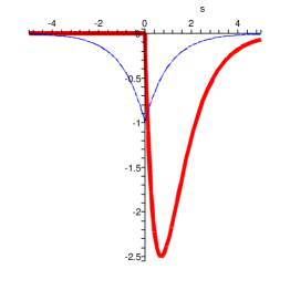
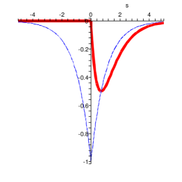
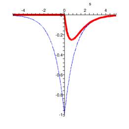
Figure 1: CH2 peakon profiles with $c=1,\rho=0.1,\>0.5,\>1$. The thick line is $u(s)$, the thin line is $v(s)$

,  

$$\left\{\begin{array}[]{l}v(r)=-\displaystyle{\frac{c^{2}}{\kappa\sqrt{\rho}}}{e^{r}},\quad r\leq r_{0}\\ v(r)=-\kappa\sqrt{\rho}{e^{(-r)}},\qquad r\geq r_{0},\end{array}\right.$$ (4.7)

In terms of the normalized variable $s=r-r_{0}$, we can compactly write this peakon solution as

$$u(s)=\displaystyle{\frac{c^{2}}{\rho}}(e^{-2s}-e^{-s})\theta(s),\>v(s)=-ce^{-|s|},\quad s=x-ct+r_{0}.$$ (4.8)

We notice that the derivatives of both $u(s)$ and $v(s)$ have a discontinuity in $s=0$ and that Rankine-Hugoniot type conditions are satisfied at $s=0$. The profile of three such peaked solutions are depicted in Figure 1.

Mimicking the Camassa-Holm original paper, we can seek for $N$-peakon solutions of CH2 by means of a linear superposition of elementary solutions of the form given by Eq. (4.8), .i.e., via the Ansatz

$$\begin{array}[]{l}u(x,t)=\sum_{i=1}^{N}\pi_{i}(t)({e^{(-2x+q_{i}(t))}}-e^{(-x+q_{i}(t))})\theta(x-q_{i}(t)),\\ v(x,t)=\sum_{i=1}^{N}-p_{i}(t)e^{(-|x-q_{i}(t)|)}.\end{array}$$ (4.9)

A tedious but straightforward computation shows the following:

Proposition 4.1

The Ansatz (4.9) gives solutions of the CH2 equation provided that the $2N$ dynamical variables $(q_{i},p_{i})$ evolve as

$$\dot{q_{i}}=\sum_{j}p_{j}{e^{(-|q_{i}-q_{j}|)}};\quad\dot{p}_{i}=p_{i}\sum_{j=1}^{N}p_{j}{e^{(-|q_{i}-q_{j}|)}}\widehat{\epsilon}_{0}(q_{i}-q_{j}),$$ (4.10)

that is, they evolve, as in the CH case [6] as canonical variables under the Hamiltonian flow of

$$H_{N}=\frac{1}{2}\sum_{i,j=1}^{N}p_{i}p_{j}{e^{(-|q_{i}-q_{j}|)}}.$$

The quantities $\pi_{i}$ can be obtained from the solutions $(q_{i}(t),p_{i}(t))_{i=1\ldots N}$ of (4.10) via the formula:

$$\pi_{i}=\displaystyle{\frac{2p_{i}}{\rho}}\sum_{j=1}^{N}p_{j}{e^{(q_{j}-q_{i})}}\widehat{\theta}_{\frac{1}{2}}(q_{i}-q_{j}).$$ (4.11)

In these formulas, $\widehat{\theta}_{\frac{1}{2}}(s)$ is the Heaviside step function with the normalization $\widehat{\theta}_{\frac{1}{2}}(0)=\frac{1}{2}$, and $\widehat{\epsilon}_{0}(s)=\widehat{\theta}_{\frac{1}{2}}(s)-\widehat{\theta}_{\frac{1}{2}}(-s)$.

Remark. The coincidence of the peakon solution of CH2 with those of CH can be, a posteriori, understood by means of the following direct link between CH2 and CH, which we report from [16]. If we apply the operator $\mathbf{1}+{\partial}_{x}$ to the first of Eq (3.13), we get

$$\begin{split}&(v-v_{xx})_{t}={\partial}_{x}(-2\rho(u+u_{x})+vv_{x}+v^{2}-(vv_{xx}+v_{x}^{2}))\\ &={\partial}_{x}(w+(\frac{3}{2}v^{2}-(\frac{1}{2}v_{x}^{2}+vv_{xx}))).\end{split}$$

Since the additional term $w$ in this equation is given by

$$w=-2\rho(u+u_{x})-\frac{1}{2}(v-v_{x})^{2}$$

we deduce the following system:

$$\begin{split}&(v-v_{xx})_{t}={\partial}_{x}(w+(\frac{3}{2}v^{2}-(\frac{1}{2}v_{x}^{2}+vv_{xx})))\\ &w_{t}=v_{t}w+2w_{t}v,\end{split}$$ (4.12)

whose consistent reduction to $w=0$ exactly gives the CH equation (2.1).

4.2 Finite gap solutions

In this Section we will address the basic properties of “finite gap” solutions of the CH2 hierarchy.

To this end, we use the Lax representation of the hierarchy, i.e., the vanishing curvature relations (see the end of Subsection 3.2)

$${\partial}_{t}L-{\partial}_{x}V+[L,V]=0,\quad\text{with }L=\left(\begin{array}[]{cc}0&1\\ \vskip 6.0pt plus 2.0pt minus 2.0pt\cr\displaystyle{{\frac{\rho\,\xi}{{\lambda}^{2}}}}&\displaystyle{{\frac{\eta}{\lambda}}}-1\end{array}\right),$$ (4.13)

and $V$ given in Eq. (3.32).

Following standard techniques in the theory of integrable systems, we consider a matrix $2\times 2$ matrix $W(\lambda)$, with elements that depend on $\lambda$, such that the Zakharov-Shabat relations

$$W(\lambda)_{x}-[L({\lambda}),W(\lambda)]=\frac{{\partial}}{{\partial}t_{W}}L(\lambda)$$ (4.14)

yield consistent equations for the variables $\eta,\xi$.

A straightforward computation shows

Proposition 4.2

To yield consistent Zakharov-Shabat equations (4.14) the matrix $W(\lambda)$ must have the form

$$W(\lambda)=\left(\begin{array}[]{cc}-\displaystyle{{\frac{\rho\,a}{\lambda}}}&b\\ \vskip 6.0pt plus 2.0pt minus 2.0pt\cr-\displaystyle{{\frac{\rho{a_{x}}}{\lambda}}}+\displaystyle{{\frac{\rho\,\xi b}{{\lambda}^{2}}}}&{b_{x}-b}+\displaystyle{{\frac{b\eta-\rho\,a}{\lambda}}}\end{array}\right),$$ (4.15)

with the ”time” evolution $\displaystyle{\frac{\partial}{\partial t_{W}}}$ given by

$${\left(\begin{array}[]{c}\displaystyle{\frac{\partial\eta}{\partial t_{W}}}\\ \displaystyle{\frac{\partial\xi}{\partial t_{W}}}\end{array}\right)}=\left(Q-\lambda P\right){\left(\begin{array}[]{c}a\\ b\end{array}\right)}$$ (4.16)

This means that $a=a(x,\lambda)$ and $b(x,\lambda)$ are obtained form the Casimir of the Poisson pencil ${\cal H}(\lambda)={\cal H}_{0}+\frac{1}{\lambda}{\cal H}_{1}+\cdots$ via:

$$a(x,\lambda)=[p(\lambda)(\displaystyle{\frac{\delta{\cal H}(\lambda)}{\delta\eta}})]_{+},\quad b(x,\lambda)=[p(\lambda)(\displaystyle{\frac{\delta{\cal H}(\lambda)}{\delta\xi}})]_{+},$$

for some polynomial (with constant coefficients) $p(\lambda)$, where $[f(\lambda)]_{+}$ represents the polynomial part in the expansion in $\lambda$ of $f(\lambda)$.

Remarks. 1) The Zakharov-Shabat representation for the times of the negative hierarchy of Subsection 3.1 can be obtained in a similar manner.
2) Eq. (3.23) with the normalization $f_{1}(\lambda)=\lambda,f_{2}(\lambda)=0$, reads $\text{Tr}(W(\lambda))=1$. Solving this for $a(x,\lambda)$, we can express every element in terms of $b(x,\lambda)$ as follows:

$$\begin{split}&W(\lambda)=\frac{1}{2}\left(\begin{array}[]{ccc}-b(x,\lambda)_{x}+b(x,\lambda)(1-\displaystyle{{\frac{\eta}{\lambda}}})-1&&2b(x,\lambda)\\ W_{2,1}&&W_{2,2}\end{array}\right),\\ &W_{2,1}=b(x,\lambda)_{x}-\,b(x,\lambda)_{x\,x}-(b(x,\lambda)\eta)_{x}/\lambda+(2\rho\,\xi\,b(x,\lambda))/\lambda^{2},\\ &W_{2,2}=b(x,\lambda)_{x}-b(x,\lambda)(1-\eta/\lambda)-1.\end{split}$$ (4.17)

3) In the notations of Section 3, the Lax representation of the $n$-th flow of the hierarchy will be obtained choosing

$$a_{n}(x,\lambda)=[\lambda^{n-1}\beta_{\eta}]_{+},b_{n}(x,\lambda)=[\lambda^{n-1}\beta_{\xi}]_{+}.$$ (4.18)

We notice that, in this way, $b_{n}(x,\lambda)$ is a monic polynomial of degree $n-1$ (while $a_{n}(x,\lambda)$ is of $n-2$). For further use we recall that, if $n\geq k$, the following relation holds, as a consequence of the definitions:

$$b_{k}(x,\lambda)=\Big{[}\displaystyle{\frac{b_{n}(x;\lambda)}{\lambda^{n-k}}}\Big{]}_{+}.$$ (4.19)

As it has been already noticed, the recurrence relations for the differentials of the Casimir function of the positive hierarchy – that is, the hierarchy to which the CH2 equations belong - cannot be solved, via local functionals in $u,v$, let alone in $\xi,\eta$. However, we can still use the Zakharov-Shabat representation of the hierarchy in the study of (some properties of) the stationary $t_{n}$ submanifolds for CH2.

Indeed, applying a scheme that dates back to [3] and has been used in [4, 5] for studying finite-gap solutions of Harry-Dym and Camassa-Holm type, we can argue as follows.

We consider $L=W_{1}$ and the matrices $W_{n}$ associated with the time $t_{n}$ of the hierarchy. On the stationary manifold of the time $t_{n}$ the matrix

$$W_{n}=\frac{1}{2}{\left(\begin{array}[]{cc}b_{n}(1-\eta/\lambda)-b_{nx}-1&2b_{n}\\ b_{nx}-b_{n\,xx}-(b_{n}\eta)_{x}/\lambda+2\rho\xi/\lambda^{2}&b_{n}(\eta/\lambda-1)+b_{nx}-1\end{array}\right)},$$ (4.20)

where $b_{n}=[\lambda^{n-1}\beta_{\xi}]_{+}$, undergoes, along the time $t_{m}$ of the hierarchy, the Lax equation

$${\frac{\partial}{\partial t_{m}}}{W_{n}}=[W_{m},W_{n}],$$ (4.21)

and so its spectral curve $\Gamma=\text{det}(\nu-W_{n}(\lambda))$, is a constant of the motion. Defining $\nu=\displaystyle{\frac{\mu-\lambda}{2\lambda}}$, $\Gamma$ is given by $\mu^{2}=R(\lambda)$, where

$$R(\lambda)=(b_{n}^{2}-2b_{n}b_{n\,xx}+b_{n\,x}^{2})\lambda^{2}-2b_{n}^{2}\big{(}(\eta-\eta_{x})\lambda-(4\rho\xi+\eta^{2})\big{)}.$$ (4.22)

We notice that, since $b_{n}$ is a monic polynomial of degree $n-1$ in $\lambda$, the degree of $R(\lambda)$ is $2n$, and so the genus of $\Gamma$ is $n-1$.

Let $(\lambda_{1},\ldots,\lambda_{n-1})$ be the $n-1$ roots of $b_{n}$, i.e, $b_{n}=\displaystyle{\prod_{j=1}^{n-1}(\lambda-\lambda_{j})}$. The $x=t_{1}$ evolution equation of these roots is governed by the equation

$$\lambda^{\prime}_{i}=\displaystyle{\frac{\partial\lambda_{i}}{\partial x}}=\displaystyle{\frac{\sqrt{(R(\lambda_{i}))}}{\lambda_{i}\prod_{j\neq i}^{n}(\lambda_{i}-\lambda_{j})}}$$ (4.23)

Moreover, thanks to the form of the matrices $W_{n}$, the Lax equations (4.21) imply that $b_{n}$ evolves along $t_{k}$ as follows

$${\frac{\partial b_{n}}{\partial t_{k}}}=b_{k}\displaystyle{\frac{\partial b_{n}}{\partial x}}-b_{n}\displaystyle{\frac{\partial b_{k}}{\partial x}},\qquad k=1,\ldots,n-1,$$ (4.24)

and so we get, evaluating these relations for $\lambda=\lambda_{i}$,

$${\frac{\partial\lambda_{i}}{\partial t_{k}}}=b_{k}(\lambda_{i})\displaystyle{\frac{\partial\lambda_{i}}{\partial x}}=b_{k}(\lambda_{i})\displaystyle{\frac{\sqrt{(R(\lambda_{i}))}}{\lambda_{i}\prod_{j\neq i}^{n}(\lambda_{i}-\lambda_{j})}}.$$ (4.25)

Since the equations (4.19) imply that $b_{k}(\lambda_{i})$ is the symmetric polynomial of order $k-1$ in $\big{(}\lambda_{1},\ldots,\lambda_{i-1},\lambda_{i+1},\ldots,\lambda_{n-1}\big{)}$ (see, e.g., [5] for the details), one arrives at the following relations

$$dt_{k}=\sum_{i=1}^{n-1}\displaystyle{\frac{\lambda_{i}^{n-k}d\lambda_{i}}{\sqrt{R(\lambda_{i})}}}.$$ (4.26)

These are non-standard Abel-Jacobi relations on the genus $g=n-1$ curve $\Gamma(\mu,\lambda)$, entailing that the third kind Abelian differential $\frac{\lambda^{g}\,d\lambda}{\sqrt{R(\lambda)}}$ is involved in the integration of the finite dimensional dynamical system associated with the stationary $t_{n}$ manifold of CH2.

4.3 The manifold $\mathbf{u=0}$ and singular solutions

The CH2 equations admit a consistent reduction to the manifold $u=0$. In this section we will show that the resulting equation, namely

$$\partial_{t}(v-v_{x})=\partial_{x}(v^{2}-vv_{x})$$ (4.27)

admit, with a suitable interpretation, non-continuous solutions, that could be called half-peakons or ”cliffon” solutions. We notice that the opportunity of studying this equation (or rather the variant of it therein considered) was suggested in [18].

We start noticing that the Green operator for $\mathbf{1}-{\partial}_{x}$ is the following:

$$G(f)(x)=\int_{x}^{\infty}{e^{x-y}}f(y)dy=\int_{-\infty}^{\infty}{e^{x-y}}\theta(y-x)f(y)dy,$$ (4.28)

where $\theta(r)$ is the Heaviside step function.

By means of this Green operator, we can rewrite Eq. (4.27) in the following integral form:

$$\partial_{t}v=\partial_{x}\big{(}\frac{v^{2}}{2}+G(\frac{v^{2}}{2})\big{)},$$ (4.29)

to be considered as the analogue of Eq. (0.1) of [17]. With the Ansatz

$$v(x,t)=A{e^{(x-ct)}}\theta(ct-x),$$ (4.30)

we get

$$\begin{split}&G(v^{2})(x)=A^{2}\,\int_{-\infty}^{\infty}{e^{(x+y-2ct)}}\theta(y-x)\theta(ct-y)dy=\\ &A^{2}\theta(ct-x)\big{(}{e^{(x-ct)}}-{e^{(2x-2ct)}}\big{)}=-v^{2}+Av.\end{split}$$ (4.31)

so that bounded traveling waves for Eq. (4.27) are of the form

$$v(x,t)=-2c{e^{(x-ct)}}\theta(ct-x),$$ (4.32)

that is, well-shaped peakons (with amplitude twice their speed), for $x<ct$ that drops to zero for $x>ct$. One can notice the same solution can be gotten from the differential equation(4.27), provided we agree to regularize the product of an Heaviside function and a Dirac $\delta$-function as $\theta(r)\delta(r)=\frac{1}{2}\delta(r)$.

The interaction of $N$ right moving cliffons can be described much in the same way of that concerning $N$ right moving peakons, described in Subsection 4.1, via the Ansatz:

$$v(x,t)=\sum_{i=1}^{N}-2p_{i}(t){e^{(x-q_{i}(t))}}\theta(q_{i}(t)-x).$$ (4.33)

One should notice the following. To evaluate $G(v^{2})$ we have to consider products

$$F_{ij}=p_{i}p_{j}{e^{(2x-q_{i}-q_{j})}}\theta(q_{i}-x)\theta(q_{j}-x).$$ (4.34)

They can be written as

$$F_{ij}=p_{i}p_{j}{e^{(2x-q_{i}-q_{j})}}\big{(}\widehat{\theta}_{\frac{1}{2}}(q_{i}-q_{j})\theta(q_{j}-x)+\widehat{\theta}_{\frac{1}{2}}(q_{j}-q_{i})\theta(q_{i}-x)\big{)},$$

where the normalized Heaviside function $\widehat{\theta}_{\frac{1}{2}}(r)$ has been defined in Proposition 4.1. Since a straightforward computation yields

$$\begin{split}G(F_{ij})(x)+F_{ij}&(x)=\\ p_{i}p_{j}\big{(}{e^{(x-q_{j})}}\theta(q_{i}-x)\widehat{\theta}_{\frac{1}{2}}(q_{j}-q_{i})&+{e^{(x-q_{i})}}\theta(q_{j}-x)\widehat{\theta}_{\frac{1}{2}}(q_{i}-q_{j})\big{)},\end{split}$$ (4.35)

we obtain that the resulting dynamical system for the $2N$ quantities $(q_{i},p_{i})$ is the following impulsive system:

$$\left\{\begin{array}[]{l}\dot{p_{i}}=0\\ \dot{q_{i}}=2\sum_{j}p_{j}{e^{q_{i}-q_{j}}}\widehat{\theta}_{\frac{1}{2}}(q_{j}-q_{i}).\end{array}\right.$$ (4.36)

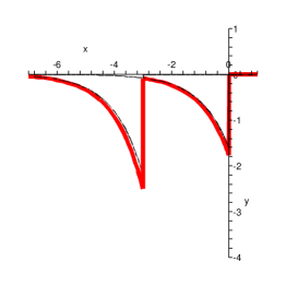
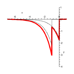
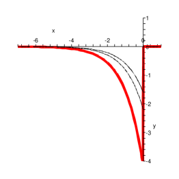
Figure 2: 2-cliffon interaction: thin lines represent the individual cliffons, while the thick one their superposition.

,  

We close the paper examining these equations of motion for a system of two cliffons, with initial conditions

$$q_{1}(0)\ll q_{2}(0),p_{1}(0)\simeq p_{2}(0)$$

For $t\simeq 0$ the evolution will be as follows (notice that $p_{i}(t)\equiv p_{i}(0)$):

$$\dot{q}_{1}=p_{1}+2p_{2}{e^{q_{1}-q_{2}}},\quad\dot{q}_{2}=p_{2}.$$

This means that the rightmost cliffon (whose tip is located at $x=q_{2}(t)$) will travel undisturbed, while the leftmost one is accelerated towards the rightmost. The initial acceleration is small, but positive. When the distance $q_{1}-q_{2}$ between the two tips is small but non zero, the acceleration of the leftmost cliffon will become sensible, so that the asymptotic equation is

$$\dot{q}_{1}\simeq p_{1}+2p_{2},\quad\dot{q}_{2}=p_{2},\quad\text{for }q_{2}-q_{1}\to 0^{+}.$$

At the moment of overtaking, however, the presence of the factor $\widehat{\theta}_{\frac{1}{2}}(q_{j}-q_{i})$ will decrease the speed of the cliffon # 1 of a factor $p_{2}$, while increasing the speed of the cliffon # 2 of a factor $p_{1}$, so that the two cliffons merge into a single one, traveling with the sum of their ”initial” speeds. This behavior is depicted in Figure 2, as seen in the reference frame of the rightmost cliffon.

Acknowledgments

The author wishes to thank B. Dubrovin, T. Grava, P. Lorenzoni, and Y. Zhang for useful discussions. He is also grateful to the organizers of SPT04 (Cala Gonone –IT, May 2004), of the Workshop Analytic and Geometric theory of the Camassa-Holm equation and Integrable Systems, (Bologna–IT, September 2004), and of the GNFM annual Meeting (Montecatini – IT, October 2004) for the possibility of presenting a few of the results herewith collected in those Conferences. This work has been partially supported by INdAM-GNFM under the research project Onde nonlineari, struttura $\tau$ e geometria delle varietà invarianti: il caso della gerarchia di Camassa-Holm, by the ESF project MISGAM, by the by the Italian M.I.U.R. under the research project Geometric methods in the theory of nonlinear waves and their applications, and by the European Community through the FP6 Marie Curie RTN ENIGMA (Contract number MRTN-CT-2004-5652).

References

- [1] S. Abenda, T. Grava, Modulation of Camassa-Holm equation and reciprocal transformations, To appear in Ann. Inst. Fourier, retrievable at http://misgam.sissa.it/?page=papers.
- [2] E. Arbarello, C. De Concini, V. Kac, C. Procesi, Moduli spaces of curves and representation theory. Comm. Math. Phys. 117 (1988), 1–36.
- [3] S.J. Alber, Investigation of equations of KdV type by the method of recurrence relations. J. Lond. Math. Soc. 19, (1979) 467–480.
- [4] M.S. Alber, R. Camassa, D.D. Holm, J.E. Marsden, The geometry of peaked solitons and billiard solution of a class of integrable PDEs, Lett. Math. Phys. 32 (1994), 137–151.
- [5] M.S. Alber, R. Camassa, Yu. N. Fedorov,D.D. Holm, J.E. Marsden, The Complex Geometry of Weak Piecewise Smooth Solution of Integrable PDEs of Shallow Water and Dym type. Comm. Math. Phys. 221 (2001), 197–227.
- [6] R. Camassa, D.D. Holm, An integrable shallow water equation with peaked solitons. Phys. Rev. Lett. 81 (1993), 1661–1664.
- [7] M. Chen, S-Q. Liu, Y. Zhang, A 2-Component Generalization of the Camassa-Holm Equation and Its Solutions, nlin.SI/0501028.
- [8] A. Degasperis, D.D. Holm, A.N.W. Hone, Integrable and non-integrable equations with peakons. Nonlinear physics: theory and experiment, II (Gallipoli, 2002), 37–43, World Sci. Publishing, River Edge, NJ, 2003.
- [9] B. Dubrovin, Y. Zhang, Normal forms of integrable PDEs, Frobenius manifolds and Gromov - Witten invariants. Book in preparation, first draft in math.DG/0108160.
- [10] B. Dubrovin, S-Q. Liu, Y. Zhang, On Hamiltonian perturbations of hyperbolic systems of conservation laws. math.DG/0410027.
- [11] B. Fuchssteiner, A.S. Fokas, Symplectic structures, their Bäcklund transformations and hereditary symmetries. Physica D, 4 (1981/82), 47–66.
- [12] I.M. Gel’fand, I. Zakharevich, On the local geometry of a bi-Hamiltonian structure. In: The Gel’fand Mathematical Seminars 1990-1992 (L. Corwin et al., eds.), Birkhäuser, Boston, 1993, pp. 51–112.
- [13] B.A. Kupershmidt, Mathematics of Dispersive Water Waves, Comm. Math. Phys. 99 (1995), 51–73
- [14] B. Khesin, G. Misiołek, Euler equations on homogeneous spaces and Virasoro orbits. Adv. Math. 176, (2003), 116–144.
- [15] Yi A. Li, P.J. Olver, P. Rosenau, Non-analytic solutions of nonlinear wave models. Nonlinear theory of generalized functions (Vienna, 1997), 129–145, Chapman & Hall/CRC Res. Notes Math., 401, Boca Raton, 1999.
- [16] S-Q. Liu, Y. Zhang, Deformations of Semisimple Bihamiltonian Structures of Hydrodynamic Type, Jour. Geom. Phys. 54 (2005), 427–453.
- [17] H. McKean, A. Constantin, The Camassa-Holm equation on the circle, Comm. Pure Appl. Math. LII, 949-982, (1999).
- [18] P.J. Olver, P. Rosenau, Tri-Hamiltonian duality between solitons and solitary waves having compact support, Phys. Rev. E., 53, 1889–1906, (1996). .