Multiple-scale analysis of discrete nonlinear partial difference equations: the reduction of the lattice potential KdV.

Abstract

We consider multiple lattices and functions defined on them. We introduce slow varying conditions for functions defined on the lattice and express the variation of a function in terms of an asymptotic expansion with respect to the slow varying lattices.

We use these results to perform the multiple–scale reduction of the lattice potential Korteweg–de Vries equation.

1 Introduction

The reductive perturbation method (or multiple–scale analysis) [18] allows us to deduce a set of simplified equations starting from a basic model without loosing its main characteristic features. The method consists essentially in an asymptotic analysis of a perturbation series, based on the existence of different scales to cure secularity.

The success of the method relies mainly on the nice property of the resulting reduced models, which are simple and often integrable. Simple here means actually simpler than the starting equations and still providing useful information. Integrable means that they carry an infinite set of conserved quantities, have an infinite set of symmetries and of exact solutions. Finally, as emphasized in [2], the reductive perturbation approach preserve integrability. Consequently this approach can be used to obtain new integrable models from known ones.

The situation is quite different in the case of differential equations on a lattice (for example, in the case of dynamical systems when one has a continuous time and discrete space variables) for which a reliable reductive perturbative method which would produce reduced discrete systems up to our knowledge does not exist. Leon and Manna [11] and later Levi and Heredero [12] proposed a set of tools which allow to perform multiple–scale analysis for a discrete evolution equation. These tools rely on the definition of a large grid scale via the comparison of the magnitude of related difference operators and on the introduction of a slow varying condition for function defined on the lattice. Their results, however, are not very promising as the reduced models are neither simpler nor more integrable than the original one. Starting from an integrable model, like the Toda lattice [19], the Leon and Manna reduction technique produce a non-integrable differential difference equation of the discrete Nonlinear Schrödinger type [13, 17]. Levi and Heredero [12] started from the integrable differential–difference Nonlinear Schrödinger equation and got a nonintegrable system of differential–difference equations of Kortewg–de Vries type.

We consider here the case of completely discrete equations defined on a two dimensional orthogonal lattice. We follow the approach introduced by Levi and Heredero [12], extended to the case of multiple orthogonal lattices. We try to keep all passages consistent with the continuous limit, when the lattice spacings on the different grids go to zero.

In Section 2 we introduce, following [12], the multiple lattices, the slow varying conditions and the asymptotic expansions of the functions’ variations while in Section 3 we apply the resulting formulas to the case of the multiple–scale expansion of the lattice potential Korteweg – de Vries equation (lpKdV) [14, 8],

$$(p-q+u_{n,m+1}-u_{n+1,m})(p+q-u_{n+1,m+1}+u_{n,m})=p^{2}-q^{2}.$$ (1)

At the end, in Section 4 we discuss the results obtained and present a list of open problems and remarks relevant also for the case of a differential–difference equation [12].

2 Multi-lattice structure and the variation of a function on them

2.1 Rescaling on the lattice

Given a lattice defined by a constant lattice spacing $h$, we will introduce an apriory infinite number of lattices defined by lattice spacings $H_{j}$, with $j=1,2,\ldots,\infty$, where $H_{j}$ are well defined functions of $h$, $H_{j}=H_{j}(h)$. In Fig. 1 we show an example of such a situation with $j=1,2$. For convenience we will denote by $n_{j}$ the running index of the points separated by $H_{j}$ and $n$ those separated by $h$. Moreover, in correspondence with the lattice variables, we can introduce the real variables $x=hn$ and $x_{j}=H_{j}n_{j}$.

A simple definition of $H_{j}$ is obtained by introducing an integer number $N$ and defining $H_{j}=N^{j}h$. If $N$ is a large number than $\frac{1}{N}=\epsilon$ will be a small number. The variables $x$ and $x_{j}$ will go over to continuous variables when respectively $h\rightarrow 0$, $n\rightarrow\infty$ and $H_{j}\rightarrow 0$, $n_{j}\rightarrow\infty$ in such a way that their products $x=nh$ and $x_{j}=n_{j}H_{j}$ are finite.

Let us assume that $x_{j}=\epsilon^{j}x$. Then, if $x\sim\frac{1}{\epsilon^{j}}$, $x_{j}\sim 1$. So $x_{j}$ represents, as $j$ increases an always larger portion of the $x$ axis. This assumption, together with the choice $\epsilon=\frac{1}{N}$, will reflect onto a relation between the lattice variables $n$ and $n_{j}$ as

$$x_{j}=H_{j}n_{j}=hN^{j}n_{j}=\epsilon^{j}x=\frac{1}{N^{j}}hn\Rightarrow n_{j}={\Bigl{[}}\frac{n}{N^{2j}}{\Bigr{]}}.$$ (2)

Consequently we need to move $N^{2j}$ points on the lattice of the discrete variable $n$ to shift the lattice variable $n_{j}$ by $1$ point.

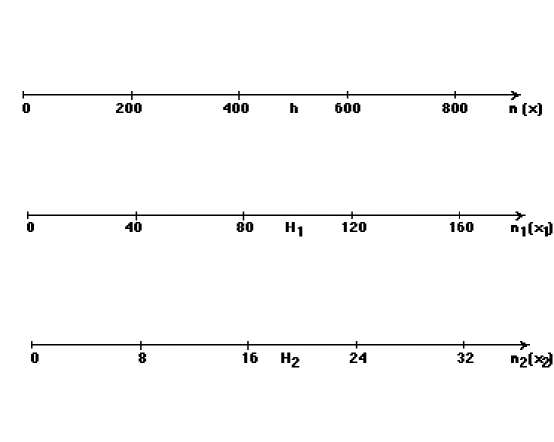
Figure 1: Multiple lattices ($n,n_{1}=\frac{n}{N},n_{2}=\frac{n}{N^{2}}$), with $N=5$; the corresponding continuous coordinate would be $x=nh$, $x_{1}=n_{1}H_{1}$ and $x_{2}=n_{2}H_{2}$ where $H_{1}=hN$, $H_{2}=hN^{2}$.

2.2 Slowly varying functions and their expansion

Here we study the relation between functions acting on the different lattices defined in Section 2.1.

Let us consider a function $f$ defined on the points of a lattice of index $n$ given in Fig. 1, i.e. $f(n)$. We are interested in understanding what happens when we assume that $f(n)=g(n_{1},n_{2},\dots,n_{K})$, i.e. $f$ depends on a finite number $K$ of slow varying lattice variables $n_{j}$ such that $g(n_{j}\pm k)=f(n\pm kN^{2j})$ (2). As we are mainly interested in applying in Section 3 these results to the lpKdV (1), we need to know what happens to the function $g$ when the function $f$ is in the point $n+1$. One needs to get explicit expressions for $f(n+1)$ in terms of $g(n_{1},n_{2},\ldots,n_{K})$ on different points in the $n_{1}$, $n_{2}$, $\ldots,n_{k}$ lattices. At first let us study the case, considered in [12] when we have only two different lattices, i.e. $K=1$. Using the results obtained in this case we will then consider the case corresponding to $K=2$. The generic case will than be obvious.

In the case of one variable we can use the result contained in [10]:

$$\Delta_{H}^{k}g(n_{1})=\sum_{i=k}^{\infty}{k!\over i!}P(i,k)\Delta^{i}_{h}f(n)$$ (3)

where $H$ is any one of the possible $H_{j}$ introduced before and $\Delta_{H}^{k}g(n_{1})=\sum_{i=0}^{k}(-1)^{k-i}{k\choose i}g(n_{1}+i)$, the $k$–variation formula obtained using a two–points forward difference scheme. The coefficients $P(i,k)$ are given by

$$P(i,j)=\sum_{\alpha=j}^{i}\left(\frac{H}{h}\right)^{\alpha}S_{i}^{\alpha}\mathfrak{S}_{\alpha}^{j}$$

with $S_{i}^{j}$, $\mathfrak{S}_{i}^{j}$ Stirling numbers of the first and second kind respectively. A table with the coefficients $P(i,k)$ for $(i,k)<(6,6)$ is contained in ref [10].

Eq. (3) allow us to express a difference of order $k$ in the lattice of spacing $H$ in terms of an infinite number of differences on the lattice of spacing $h$. To get an approximate solution we have to truncate the expansion at the r.h.s. of eq. (3) by requiring a slow varying condition for the function $f(n)$. We will say that the function $f(n)$ is a slow varying function of order $p$ if $\Delta^{p+1}_{h}f(n)=0.$ A slow varying function of order $p$ is a polynomial of degree $p$ in $n$ [5]. For a function of order  $p=1$, eq. (3) reduces to

$$\Delta_{H}g(n_{1})=N^{2}\Delta_{h}f(n).$$ (4)

Dividing eq. (4) by $h$ and taking the limit as $h\rightarrow 0$, with $x=hn$ and $x_{1}=n_{1}H_{1}=n_{1}hN$ finite, we get $\frac{df(x)}{dx}=\epsilon\frac{dg(x_{1})}{dx_{1}}$. In the case $p=2$, we get:

$$\Delta^{2}_{H}g(n_{1})=N^{4}\Delta^{2}_{h}f(n),$$ (5)

$$\Delta_{H}g(n_{1})=N^{2}\Delta_{h}f(n)+\frac{N^{2}(N^{2}-1)}{2}\Delta^{2}_{h}f(n).$$ (6)

For $p=3$ we have

$$\Delta^{3}_{H}g(n_{1})=N^{6}\Delta^{3}_{h}f(n),$$

$$\Delta^{2}_{H}g(n_{1})=N^{4}\Delta^{2}_{h}f(n)+N^{4}(N^{2}-1)\Delta^{3}_{h}f(n),$$

$$\Delta_{H}g(n_{1})=N^{2}\Delta_{h}f(n)+\frac{N^{2}(N^{2}-1)}{2}\Delta^{2}_{h}f(n)+\frac{N^{2}(N^{2}-1)(N^{2}-2)}{6}\Delta^{3}_{h}f(n),$$

and for $p=4$ we have:

$$\Delta^{4}_{H}g(n_{1})=N^{8}\Delta^{4}_{h}f(n),$$ (7)

$$\Delta^{3}_{H}g(n_{1})=N^{6}\Delta^{2}_{h}f(n)+\frac{3N^{6}(N^{2}-1)}{2}\Delta^{4}_{h}f(n),$$

$$\Delta_{H}^{2}g(n_{1})=N^{4}\Delta_{h}^{2}f(n)+N^{4}(N^{2}-1)\Delta^{3}_{h}f(n)+$$

$$\qquad+[\frac{7}{12}N^{6}(N^{2}-1)-\frac{11}{12}N^{4}(N^{2}-1)]\Delta^{4}_{h}f(n),$$

$$\Delta_{H}g(n_{1})=N^{2}\Delta_{h}f(n)+\frac{1}{2!}N^{2}(N^{2}-1)\Delta^{2}_{h}f(n)+$$

$$+\frac{1}{3!}N^{2}(N^{2}-1)(N^{2}-2)\Delta^{3}_{h}f(n)+\frac{1}{4!}N^{2}(N^{2}-1)(N^{2}-2)(N^{2}-3)\Delta^{4}_{h}f(n).$$

From (4), if $f(n)$ is a slow function of order 1, $f(n+1)$ reads:

$$f(n+1)=g(n_{1})+\frac{1}{N^{2}}[g(n_{1}+1)-g(n_{1})]+o(\frac{1}{N^{4}}),$$ (8)

while, if the function $f(n)$ is a slow varying function of order 2, $f(n+1)$ is given by

$$f(n+1) = g(n_{1})+\frac{1}{2N^{2}}[-g(n_{1}+2)+4g(n_{1}+1)-3g(n_{1})]+$$

$$+ \frac{1}{2N^{4}}[g(n_{1}+2)-2g(n_{1}+1)+g(n_{1})]+o(\frac{1}{N^{6}}).$$

When the function $f(n$) is a slow varying function of order 3, $f(n+1)$ is given by

$$f(n+1) = g(n_{1})+\frac{1}{6N^{2}}[2g(n_{1}+3)-9g(n_{1}+2)+13g(n_{1}+1)-6g(n_{1})]+$$

$$+ \frac{1}{2N^{4}}[-g(n_{1}+3)+4g(n_{1}+2)-5g(n_{1}+1)+2g(n_{1})]+$$

$$+ \frac{1}{6N^{6}}[g(n_{1}+3)-3g(n_{1}+2)+3g(n_{1}+1)-g(n_{1})]+o(\frac{1}{N^{8}}),$$

and, when the function $f(n)$ is a slow varying function of order 4, is given

$$f(n+1)=g(n_{1})+$$ (11)

$$+\frac{1}{12N^{2}}[-3g(n_{1}+4)+16g(n_{1}+3)-36g(n_{1}+2)+48g(n_{1}+1)-25g(n_{1})]+$$

$$+\frac{1}{24N^{4}}[11g(n_{1}+4)-56g(n_{1}+3)+114g(n_{1}+2)-104g(n_{1}+1)+35g(n_{1})]+$$

$$+\frac{1}{12N^{6}}[-3g(n_{1}+4)+14g(n_{1}+3)-24g(n_{1}+2)+18g(n_{1}+1)-5g(n_{1})]+$$

$$+\frac{1}{24N^{8}}[g(n_{1}+4)-4g(n_{1}+3)+6g(n_{1}+2)-4g(n_{1}+1)+g(n_{1})]+o(\frac{1}{N^{10}}).$$

In Section 3 we consider the reduction of an integrable discrete equation and will be interested in obtaining from it integrable discrete equations. It is known [20] that a scalar differential difference equation can possess higher conservation laws and thus be integrable only if it depends symmetrically on the discrete variable, i.e. if the discrete equation is invariant with respect to the inversion of $n$. So we will choose asymptotic discrete formulas which contain both $f(n\pm 1)$. The results contained in eq. (3) do not provide us with centralized formulas. To get symmetric formulas we need to take into account the following observations:

1. Eq. (3) is valid also if $H$ and $h$ are both negative;

2. For a slow varying function of order $p$, $\Delta_{h}^{p}f(n)=\Delta_{h}^{p}f(n+l)$ for any integer number $l$.

Using these observations, from eq. (8) we get

$$f(n-1)=g(n_{1})+\frac{1}{N^{2}}[g(n_{1}-1)-g(n_{1})]+o(\frac{1}{N^{4}}),$$ (12)

and in place of eq. (2.2) we have

$$f(n+1) = g(n_{1})+\frac{1}{2N^{2}}[g(n_{1}+1)-g(n_{1}-1)]+$$ (13)

$$+ \frac{1}{2N^{4}}[g(n_{1}+1)-2g(n_{1})+g(n_{1}-1)]+o(\frac{1}{N^{6}}),$$

when the function $f(n)$ is a slow varying function of order 2. To get eq. (13) we have to write, using Observation 2, eqs. (5, 6) in the form

$$\Delta_{H}^{2}g(n_{1})=N^{4}{\tilde{\Delta}}^{2}_{h}f(n),$$ (14)

$$\Delta_{H}g(n_{1})=N^{2}\Delta_{h}f(n)+\frac{N^{2}(N^{2}-1)}{2}{\tilde{\Delta}}^{2}_{h}f(n),$$ (15)

where by the symbol $\tilde{\Delta}$ we mean the centralized version of the difference operator. In the case of eq. (14, 15) ${\tilde{\Delta}}^{2}_{h}f(n)=f(n+1)-2f(n)+f(n-1)$.

When $f(n)$ is a slow varying function of odd order we are not able to construct completely symmetric derivatives using just two points forward difference formulas and thus $f(n+1)$ and $f(n-1)$ will never be expressed in a symmetric form (see for example eqs. (8, 12)). In the case when the function $f(n)$ is a slow varying function of order 4, we have to rewrite formulas (7) using both observations introduced before. We have:

$${\tilde{\Delta}}^{4}_{H}g(n_{1})=N^{8}{\tilde{\Delta}}^{4}_{h}f(n),$$ (16)

$${\tilde{\Delta}}^{2}_{H}g(n_{1})=N^{4}{\tilde{\Delta}}^{2}_{h}f(n)+\frac{N^{4}(N^{4}-1)}{12}{\tilde{\Delta}}^{4}_{h}f(n),$$

$$\Delta_{H}^{2}g(n_{1})=N^{4}\Delta_{h}^{2}f(n)+N^{4}(N^{2}-1){\hat{\Delta}}^{3}_{h}f(n)+$$

$$\qquad+[\frac{7}{12}N^{6}(N^{2}-1)-\frac{11}{12}N^{4}(N^{2}-1)]{\tilde{\Delta}}^{4}_{h}f(n),$$

$$\Delta_{H}g(n_{1})=N^{2}\Delta_{h}f(n)+\frac{1}{3!}N^{2}(N^{2}-1)(N^{2}-2){\hat{\Delta}}^{3}_{h}f(n)+$$

$$+\frac{1}{2!}N^{2}(N^{2}-1)\Delta^{2}_{h}f(n)+\frac{1}{4!}N^{2}(N^{2}-1)(N^{2}-2)(N^{2}-3){\tilde{\Delta}}^{4}_{h}f(n).$$

where, using Observation 2, we have written $\Delta^{3}_{h}f(n)$ as ${\hat{\Delta}}^{3}_{h}f(n)=2f(n+2)-7f(n+1)+9f(n)-5f(n-1)+f(n-2)$. Inverting formulas (16) we have:

$$f(n+1)=g(n_{1})-\frac{1}{12N^{2}}[g(n_{1}+2)-8g(n_{1}+1)+8g(n_{1}-1)-g(n_{1}-2)]$$ (17)

$$-\frac{1}{24N^{4}}[g(n_{1}+2)-16g(n_{1}+1)+30g(n_{1})-16g(n_{1}-1)+g(n_{1}-2)]$$

$$+\frac{1}{12N^{6}}[g(n_{1}+2)-2g(n_{1}+1)+2g(n_{1}-1)-g(n_{1}-2)]+$$

$$\frac{1}{24N^{8}}[g(n_{1}+2)-4g(n_{1}+1)+6g(n_{1})-4g(n_{1}-1)+g(n_{1}-2)]+o(\frac{1}{N^{10}}).$$

Let us pass now to the case of functions of multiple variables, i.e. when $g=g(n_{1},n_{2},\ldots,n_{K})$. If $n_{1}$, $n_{2}$, …, $n_{K}$ were completely independent discrete variables than any operation on one of the variables will not reflect on the other. If, however we have $f(n)=g(n_{1},n_{2},\ldots,n_{K})$ and $n_{j}=\frac{n}{N^{2j}}$, then any shift of $n$ will reflect on all variables $n_{1}$, $n_{2}$, …, $n_{K}$. We will consider later the case when the multiple variables are independent, i.e. the partial difference case.

Let us consider here in all details the case of $K=2$, which is the case we will need in the Section 3. $f(n)=g(n_{1},n_{2})$ and we are looking for a representation of $f(n+1)$ in terms of $g(n_{1},n_{2})$ and its shifted values. The resulting formulas will depend in a crucial way on the slow varying order of the function $f(n)$ with respect to $n_{1}$ and $n_{2}$. If the variation of both variables has to appear in the expansion of $f(n+1)$ than the slow varying order with respect to $n_{1}$ must be greater than that of $n_{2}$. $f(n)$ cannot be a slow varying function of order 1 in $n_{1}$ as in this case $f(n+1)$ will have no variation in $n_{2}$. If $f(n)$ is a slow varying function of order 2 in $n_{1}$ than it can be either of order 1 or 2 in $n_{2}$. In both cases the obtained formula will be valid up to order $\frac{1}{N^{4}}$, but, in the first case the obtained expression will not be symmetric in $n_{2}$. When $f(n)$ is a slow varying function of order 2 in $n_{1}$ and of order 1 in $n_{2}$, taking into account eqs. (15, 4) and the observation given before, we have:

$$g(n_{1}+1,n_{2})=g(n_{1},n_{2})+N^{2}[f(n+1,n_{2})-f(n,n_{2})]+$$ (18a)

$$+\frac{N^{2}(N^{2}-1)}{2}[f(n+1,n_{2})-2f(n,n_{2})+f(n-1,n_{2})],$$

$$g(n_{1}-1,n_{2})=g(n_{1},n_{2})-N^{2}[f(n+1,n_{2})-f(n,n_{2})]+$$ (18b)

$$+\frac{N^{2}(N^{2}-1)}{2}[f(n+1,n_{2})-2f(n,n_{2})+f(n-1,n_{2})],$$

$$g(n_{1},n_{2}+1)=g(n_{1},n_{2})+N^{4}[f(n_{1},n+1)-f(n_{1},n)],$$ (18c)

$$g(n_{1}+1,n_{2}+1)=g(n_{1},n_{2}+1)+N^{2}[f(n+1,n_{2}+1)-f(n_{1},n_{2}+1)]+$$ (18d)

$$+\frac{N^{2}(N^{2}-1)}{2}[f(n+1,n_{2}+1)-2f(n_{1},n_{2}+1)+f(n-1,n_{2}+1)],$$

$$g(n_{1}-1,n_{2}+1)=g(n_{1},n_{2}+1)-N^{2}[f(n+1,n_{2}+1)-f(n_{1},n_{2}+1)]+$$ (18e)

$$+\frac{N^{2}(N^{2}-1)}{2}[f(n+1,n_{2}+1)-2f(n_{1},n_{2}+1)+f(n-1,n_{2}+1)],$$

where we took into account that on the unshifted point $n=n_{1}=n_{2}$, $f(n)=f(n,n_{2})=f(n_{1},n)=f(n,n)=g(n_{1},n_{2})$ and that $f(n+1,n_{2}+1)$, which is appearing in eqs. (18d, 18e), is obtained from $g(n_{1},n_{2}+1)$, given by eq. (18c), by substituting $n_{1}$ by $n+1$. In such a way the 5 variables on the l.h.s. of eqs. (18) are expressed in terms of the 6 variables $f(n)$, $f(n+1)=f(n+1,n+1)$, $f(n_{1},n+1)=f(n,n+1)$, $f(n\pm 1,n_{2})=f(n\pm 1,n)$, $f(n-1,n+1)$ appearing on the r.h.s. of eqs. (18). Let us notice that to get a coherent number of equations with respect to the unknowns we had to consider also eqs. (18b, 18e) which involve $n_{1}-1$. We can invert the system (18) and get:

$$f(n+1)=g(n_{1},n_{2})+\frac{1}{2N^{2}}[g(n_{1}+1,n_{2})-g(n_{1}-1,n_{2})]+$$ (19)

$$+\frac{1}{N^{4}}[g(n_{1},n_{2}+1)-g(n_{1},n_{2})]+$$

$$+\frac{1}{2N^{4}}\{[g(n_{1}-1,n_{2})-2g(n_{1},n_{2})+g(n_{1}+1,n_{2})]\}+o(\frac{1}{N^{6}}).$$

In the continuous limit, when $n\rightarrow\infty$ and $h\rightarrow 0$ in such a way that $nh\rightarrow x$, eq. (19) will give

$$f_{,x}(x)=\epsilon g_{,x_{1}}(x_{1},x_{2})+\epsilon^{2}g_{,x_{2}}(x_{1},x_{2}).$$ (20)

When $f(n)$ is a slow varying function of second order in both variables, in place of eq. (18) we have:

$$g(n_{1}+1,n_{2})=g(n_{1},n_{2})+N^{2}[f(n+1,n_{2})-f(n,n_{2})]+$$ (21a)

$$+\frac{N^{2}(N^{2}-1)}{2}[f(n+1,n_{2})-2f(n,n_{2})+f(n-1,n_{2})],$$

$$g(n_{1}-1,n_{2})=g(n_{1},n_{2})-N^{2}[f(n+1,n_{2})-f(n,n_{2})]+$$ (21b)

$$+\frac{N^{2}(N^{2}-1)}{2}[f(n+1,n_{2})-2f(n,n_{2})+f(n-1,n_{2})],$$

$$g(n_{1},n_{2}+1)=g(n_{1},n_{2})+N^{4}[f(n_{1},n+1)-f(n_{1},n)]+$$ (21c)

$$+\frac{N^{4}(N^{4}-1)}{2}[f(n_{1},n+1)-2f(n_{1},n)+f(n_{1},n-1)],$$

$$g(n_{1},n_{2}-1)=g(n_{1},n_{2})-N^{4}[f(n_{1},n+1)-f(n_{1},n)]+$$ (21d)

$$+\frac{N^{4}(N^{4}-1)}{2}[f(n_{1},n+1)-2f(n_{1},n)+f(n_{1},n-1)],$$

$$g(n_{1}+1,n_{2}+1)=g(n_{1},n_{2}+1)+N^{2}[f(n+1,n_{2}+1)-f(n_{1},n_{2}+1)]+$$ (21e)

$$+\frac{N^{2}(N^{2}-1)}{2}[f(n+1,n_{2}+1)-2f(n_{1},n_{2}+1)+f(n-1,n_{2}+1)],$$

$$g(n_{1}-1,n_{2}+1)=g(n_{1},n_{2}+1)-N^{2}[f(n+1,n_{2}+1)-f(n_{1},n_{2}+1)]+$$ (21f)

$$+\frac{N^{2}(N^{2}-1)}{2}[f(n+1,n_{2}+1)-2f(n_{1},n_{2}+1)+f(n-1,n_{2}+1)],$$

$$g(n_{1}+1,n_{2}-1)=g(n_{1},n_{2}-1)+N^{2}[f(n+1,n_{2}-1)-f(n_{1},n_{2}-1)]+$$ (21g)

$$+\frac{N^{2}(N^{2}-1)}{2}[f(n+1,n_{2}-1)-2f(n_{1},n_{2}-1)+f(n-1,n_{2}-1)],$$

$$g(n_{1}-1,n_{2}-1)=g(n_{1},n_{2}-1)-N^{2}[f(n+1,n_{2}-1)-f(n_{1},n_{2}-1)]+$$ (21h)

$$+\frac{N^{2}(N^{2}-1)}{2}[f(n+1,n_{2}-1)-2f(n_{1},n_{2}-1)+f(n-1,n_{2}-1)].$$

In this case the 8 variables on the l.h.s. of eqs. (21) are expressed in terms of the 9 variables $f(n)=f(n,n)$, $f(n\pm 1)=f(n\pm 1,n\pm 1)$, $f(n_{1},n\pm 1)=f(n,n\pm 1)$, $f(n\pm 1,n_{2})=f(n\pm 1,n)$, $f(n-1,n+1)$ and $f(n+1,n-1)$ appearing on the r.h.s. of eqs. (21). One can invert the system (21) and gets:

$$f(n+1) = g(n_{1},n_{2})+\frac{1}{2N^{2}}[g(n_{1}+1,n_{2})-g(n_{1}-1,n_{2})]+$$

$$+ \frac{1}{2N^{4}}[g(n_{1}-1,n_{2})-2g(n_{1},n_{2})+g(n_{1}+1,n_{2})]+$$

$$+ \frac{1}{2N^{4}}[g(n_{1},n_{2}+1)-g(n_{1},n_{2}-1)]+o(\frac{1}{N^{6}}).$$

In the continuous limit, when $n\rightarrow\infty$ and $h\rightarrow 0$ in such a way that $nh\rightarrow x$, eq. (2.2) will give eq. (20).

Let us write here just the final result when $f(n)=g(n_{1},n_{3})$ is of order 4 in the variable $n_{1}$ and of order 2 in $n_{3}$. We have:

$$f(n+1)=g(n_{1},n_{3})-$$ (23)

$$-\frac{1}{12N^{2}}[g(n_{1}+2,n_{3})-8g(n_{1}+1,n_{3})+8g(n_{1}-1,n_{3})-g(n_{1}-2,n_{3})]+$$

$$+\frac{1}{24N^{4}}[g(n_{1}+2,n_{3})-16g(n_{1}+1,n_{3})+30g(n_{1},n_{3})-16g(n_{1}-1,n_{3})+$$

$$+g(n_{1}-2,n_{3})]+\frac{1}{2N^{6}}[g(n_{1},n_{3}+1)-g(n_{1},n_{3}-1)]-\frac{1}{12N^{6}}[g(n_{1}+2,n_{3})$$

$$-2g(n_{1}+1,n_{3})+2g(n_{1}-1,n_{3})-g(n_{1}-2,n_{3})]+o(\frac{1}{N^{8}}).$$

In the continuous limit, when when $n\rightarrow\infty$ and $h\rightarrow 0$ in such a way that $nh\rightarrow x$, eq. (23) will give

$$f_{,x}(x)=\epsilon g_{,x_{1}}(x_{1},x_{3})+\epsilon^{3}g_{,x_{3}}(x_{1},x_{3}).$$ (24)

One can introduce constant parameters in the definition of $n_{1}$, $n_{2}$ or $n_{3}$ in terms of $n$. For example we can write $n_{1}=\frac{nM_{1}}{N^{2}}$ and $n_{2}=\frac{nM_{2}}{N^{4}}$. $M_{1}$ and $M_{2}$ cannot be completely arbitrary as $n_{1}$, $n_{2}$, $n$ and $N$ are integers. In such a case eq. (19) reads:

$$f(n+1) = g(n_{1},n_{2})+\frac{M_{1}}{2N^{2}}[g(n_{1}+1,n_{2})-g(n_{1}-1,n_{2})]+$$

$$+ \frac{M_{2}}{N^{4}}[g(n_{1},n_{2}+1)-g(n_{1},n_{2})]+$$

$$+ \frac{M_{1}^{2}}{2N^{4}}\{[g(n_{1}-1,n_{2})-2g(n_{1},n_{2})+g(n_{1}+1,n_{2})]\}+o(\frac{1}{N^{6}}).$$

In Section 3 we will apply these results to a partial difference equation. For the sake of simplicity from now on we write the independent variables as indices. For completeness, in the following we present the formulas for two independent lattices, $n$ and $m$, and a function defined on them $f_{n,m}$. As the two lattices are independent the formulas presented above apply independently on each of the lattice variables. So, for example, $f_{n+1,m}$ when the function $f$ is a slowly varying function of order 2 of a lattice variable $n_{1}$ (see eq. (13) ) will read:

$$f_{n+1,m} = g_{n_{1},m}+\frac{1}{2N^{2}}[g_{n_{1}+1,m}-g_{n_{1}-1,m}]+$$

$$+ \frac{1}{2N^{4}}[g_{n_{1}+1,m}-2g_{n_{1},m}+g_{n_{1}-1,m}]+o(\frac{1}{N^{6}}),$$

and similarly for a variation with respect to $m$ alone or to the case when we will introduce multiple lattices associated to $n$ or $m$, when formulas (19, 2.2, 23) are to be taken into account. A slightly less obvious situation appears when we consider $f_{n+1,m+1}$, as new terms will appear. We consider here just the case we will need later when $n_{1}=\frac{M_{1}n}{N^{2}}$, $m_{1}=\frac{M_{2}m}{N^{2}}$ and $m_{2}=\frac{n}{N^{4}}$. If $f$ is a slow varying function of first order in $m_{2}$ and of second order in both $n_{1}$ and $m_{1}$, $f_{n+1,m+1}$ reads:

$$f_{n+1,m+1} = g_{n_{1},m_{1},m_{2}}+\frac{M_{1}}{2N^{2}}[g_{n_{1}+1,m_{1},m_{2}}-g_{n_{1}-1,m_{1},m_{2}}]+$$

$$+ \frac{M_{2}}{2N^{2}}[g_{n_{1},m_{1}+1,m_{2}}-g_{n_{1},m_{1}-1,m_{2}}]+$$

$$+ \frac{M_{1}^{2}}{2N^{4}}[g_{n_{1}+1,m_{1},m_{2}}+g_{n_{1}-1,m_{1},m_{2}}-2g_{n_{1},m_{1},m_{2}}]+$$

$$+ \frac{M_{2}^{2}}{2N^{4}}[g_{n_{1},m_{1}+1,m_{2}}+g_{n_{1},m_{1}-1,m_{2}}-2g_{n_{1},m_{1},m_{2}}]+$$

$$+ \frac{M_{1}M_{2}}{4N^{4}}[g_{n_{1}+1,m_{1}+1,m_{2}}+g_{n_{1}-1,m_{1}-1,m_{2}}-g_{n_{1}+1,m_{1}-1,m_{2}}-$$

$$- g_{n_{1}-1,m_{1}+1,m_{2}}]+\frac{1}{N^{4}}[g_{n_{1},m_{1},m_{2}+1}-g_{n_{1},m_{1},m_{2}}]+o(\frac{1}{N^{6}}).$$

As one can see in its fifth and sixth lines, eq. (2.2) contains extra terms involving variations in both the $m_{1}$ and the $n_{1}$ lattices.

3 Reduction of the lattice potential KdV

In this Section we apply the results presented in Section 2 to the case of the lattice potential KdV (1). By expanding the left hand side of eq. (1), one separates the linear and nonlinear parts:

$$(p-q)(u_{n+1,m+1}-u_{n,m})+(p+q)(u_{n+1,m}-u_{n,m+1})=$$ (28)

$$(u_{n+1,m}-u_{n,m+1})(u_{n+1,m+1}-u_{n,m}).$$

This equation involves just four points which lay on two orthogonal infinite lattices and are the vertices of an elementary square.

Let us solve the linear equation

$$F=(p-q)(u_{n+1,m+1}-u_{n,m})+(p+q)(u_{n+1,m}-u_{n,m+1})=0.$$ (29)

The discrete Fourier transform [5] will reduce the solution of the Partial Difference Equation (P$\Delta$E) (29) to that of an ordinary difference equation. Defining:

$$u_{n,m} = \frac{1}{2\pi i}\oint_{{\cal C}_{1}}v_{m}(z)z^{n-1}dz,$$ (30)

$$v_{m}(z) = \sum_{n=-\infty}^{+\infty}u_{n,m}~{}z^{-n},$$ (31)

where ${\cal C}_{1}$ is the unit circle, we reduce equation (29) to the following first order equation for $v_{m}(z)$

$$v_{m+1}(z)[(p-q)z-(p+q)]-v_{m}(z)[(p-q)-z(p+q)]=0,$$ (32)

whose solution is given by

$$v_{m}(z)={\Bigl{[}}\frac{(p-q)-z(p+q)}{(p-q)z-(p+q)}{\Bigr{]}}^{m}v_{0}(z).$$ (33)

Given any initial condition $u_{n,0}$ the general solution of (29) is given by

$$u_{n,m}=\frac{1}{2\pi i}\sum_{j=-\infty}^{+\infty}u_{j,0}\oint_{{\cal C}_{1}}{\Bigl{[}}\frac{(p-q)-z(p+q)}{(p-q)z-(p+q)}{\Bigr{]}}^{m}~{}z^{n-j-1}dz.$$ (34)

Eqs. (30, 34) can be rewritten in a more natural way (from the continuous point of view) by defining

$$z=e^{ik};\qquad\Omega=e^{-i\omega}={\Bigl{[}}\frac{(p-q)-z(p+q)}{(p-q)z-(p+q)}{\Bigr{]}}.$$ (35)

In such a case eq. (30) is just the standard Fourier transform and the solution (34) is just written as a superposition of linear waves. The dispersion relation for these linear waves is given by $\omega=\omega(k)$ and reads:

$$\omega=-2\arctan{\Bigl{[}}\frac{p}{q}\tan{\Bigl{(}}\frac{k}{2}{\Bigr{)}}{\Bigr{]}}.$$ (36)

In the following, however, to avoid too complicate formulas we express the solutions of the linear equation in term of $z$ and $\Omega$.

The lpKdV is an integrable equation of the same category of the KdV [3] as it possesses a Lax pair [15] which can be obtained by requiring that the model be consistent around a cube. So, as from KdV we get by multiple-scale reduction the NLS [21], the same we may expect here [2]. To get an integrable discrete equation we expect a resulting discrete equation which is somehow symmetric. At least when $h_{t}\rightarrow 0$ with $t=mh_{t}$ the differential difference equation we obtain must be symmetric in terms of the inversion of $n_{j}$ [20], i.e. if it depends on $n_{j+k}$ it will depend in the same way on $n_{j-k}$. So in the transformation of the discrete dependent variables we prefere to use formulas (13, 17) for the space variables, while considering the lowest possible approximation for the discrete time variable (8). So, in the multiple–scale expansion, as we do not need to have the discrete time variable appearing in a symmetric way, we use eqs. (19).

Taking into account eq. (34), we consider a wave solution of eq. ( 29) given by

$$E_{n,m}=e^{i(kn-\omega(k)m)}=z^{n}\Omega^{m}.$$ (37)

Eq. (37) solves $F=0$ if $\omega$ is given by eq. (36). Then we look for solutions of eq. (28) written as a combination of modulated waves:

$$u_{n,m}=\sum_{s=0}^{+\infty}\varepsilon^{\beta_{s}}\psi^{(s)}_{n_{1},m_{1},m_{2}}(E_{n,m})^{s}+$$ (38)

$$+\sum_{s=0}^{+\infty}\varepsilon^{\beta_{s}}{\bar{\psi}}^{(s)}_{n_{1},m_{1},m_{2}}({\bar{E}}_{n,m})^{s}$$

where $\psi^{(s)}_{n_{1},m_{1},m_{2}}$ are slowly varying functions on the lattice and $\varepsilon=N^{-2}$. By $\bar{a}$ we mean the complex conjugate of $a$ so that, for example, ${\bar{E}}_{n,m}=e^{-i(kn-\omega(k)m)}=(E_{n,m})^{-1}$, and the positive numbers $\beta_{s}$ are such that $\beta_{0}=1$ and $\beta_{j}=j$. The discrete slow varying variables $n_{1}$, $m_{1}$ and $m_{2}$ are defined in terms of $n$ and $m$ by

$$n = n_{1}\frac{N^{2}}{M_{1}},$$

$$m = m_{1}\frac{N^{2}}{M_{2}},$$ (39)

$$m = m_{2}N^{4}.$$

Eq. (39) is meaningful if $M_{1}$ and $M_{2}$ are divisors of $N^{2}$.

Introducing the expansion (38) into eq. (28) and picking out the coefficients of the various harmonics $(E_{n,m})^{s}$ we get a set of determining equations. For $s=1$, having defined $\psi^{(1)}=\psi$, we get at lowest order in $\varepsilon$:

$$\psi_{n_{1},m_{1},m_{2}}{\Bigl{[}}(q-p)(1-z\Omega)-(p+q)(\Omega-z){\Bigr{]}}=0,$$ (40)

which is identically solved by the dispersion relation (36). At $\varepsilon^{2}$ we get a linear equation

$$M_{2}{\Bigl{[}}(p-q)z\Omega-(p+q)\Omega){\Bigr{]}}{\Bigl{[}}\psi_{n_{1},m_{1}+1,m_{2}}-\psi_{n_{1},m_{1}-1,m_{2}}{\Bigr{]}}+$$ (41)

$$+M_{1}{\Bigl{[}}(p-q)z\Omega+(p+q)z{\Bigr{]}}{\Bigl{[}}\psi_{n_{1}+1,m_{1},m_{2}}-\psi_{n_{1}-1,m_{1},m_{2}}{\Bigr{]}}=0$$

whose solution is given by choosing

$$\psi_{n_{1},m_{1},m_{2}}=\phi_{n_{2},m_{2}}$$ (42)

where

$$n_{2}=n_{1}-m_{1}.$$ (43)

The solution (42) is obtained by choosing the integers $M_{1}$ and $M_{2}$ as

$$M_{1}=S~{}\Omega{\Bigl{[}}(p-q)z-(p+q){\Bigr{]}},$$ (44)

$$M_{2}=S~{}z{\Bigl{[}}(p-q)\Omega+(p+q){\Bigr{]}},$$

where $S$ is an arbitrary complex constant. Let us notice that also $n_{2}=n_{1}+m_{1}$ solves eq. (43) by an appropriate choice of $M_{1}$ and $M_{2}$. Moreover, $\frac{M_{1}}{M_{2}}=\omega_{,k}$, the group velocity. As $M_{1}$ and $M_{2}$ are integers, not all values of $k$ are admissible as $\omega_{,k}$ must be a rational number.

At $\varepsilon^{3}$ we get a nonlinear equation for $\phi_{n_{2},m_{2}}$ which depends on $\psi^{(2)}_{n_{2},m_{2}}$ and $\psi^{(0)}_{n_{2}+1,m_{2}}-\psi^{(0)}_{n_{2}-1,m_{2}}$:

$$c_{1}(\phi_{n_{2},m_{2}+1}-\phi_{n_{2},m_{2}})+c_{2}(\phi_{n_{2}+2,m_{2}}+\phi_{n_{2}-2,m_{2}}-2\phi_{n_{2},m_{2}})+$$ (45)

$$+c_{3}(\phi_{n_{2}+1,m_{2}}+\phi_{n_{2}-1,m_{2}}-2\phi_{n_{2},m_{2}})+c_{4}\phi_{n_{2},m_{2}}(\psi^{(0)}_{n_{2}+1,m_{2}}-\psi^{(0)}_{n_{2}-1,m_{2}})+$$

$$+c_{5}\psi^{(2)}_{n_{2},m_{2}}{\bar{\phi}}_{n_{2},m_{2}}=0,$$

where

$$c_{1} = [(p-q)-z(p+q)],$$

$$c_{2} = S^{2}z^{2}pq(p-q){\Bigl{[}}\frac{(p+q)z-(p-q)}{(p+q)-z(p-q)}{\Bigr{]}}^{2},$$

$$c_{3} = -2S^{2}zpq(p-q)\frac{[z(p+q)-(p-q)][(z^{2}+1)(p+q)-2(p-q)]}{[(p+q)-z(p-q)]^{2}},$$

$$c_{4} = -2S^{2}(p^{2}-q^{2})(z^{2}-1){\Bigl{[}}\frac{z+1}{(p+q)-z(p-q)}{\Bigr{]}}^{2},$$

$$c_{5} = -2\frac{q(p^{2}-q^{2})}{z[(p+q)z-(p-q)]}{\Bigl{[}}\frac{(z+1)(z^{2}-1)}{(p+q)-z(p-q)}{\Bigr{]}}^{2}.$$

The lowest order equations for the harmonics $s=0$ and $s=2$ appear at $\varepsilon^{2}$ and give:

$$\psi^{(0)}_{n_{2}+1,m_{2}}-\psi^{(0)}_{n_{2}-1,m_{2}}=2|\phi_{n_{2},m_{2}}|^{2}\frac{(1+z)^{2}}{Spz[(p+q)z-(p-q)]},$$ (46)

$$\psi^{(2)}_{n_{2},m_{2}}=(\phi_{n_{2},m_{2}})^{2}\frac{1+z}{2p(1-z)}.$$ (47)

Taking these results into account the nonlinear equation (45) for $\phi_{n_{2},m_{2}}$ reads:

$$i{\Bigl{[}}\phi_{n_{2},m_{2}+1}-\phi_{n_{2},m_{2}}{\Bigr{]}}=C_{1}(k){\Bigl{[}}\phi_{n_{2}+2,m_{2}}+\phi_{n_{2}-2,m_{2}}-2\phi_{n_{2},m_{2}}{\Bigr{]}}+$$ (48)

$$+C_{2}(k){\Bigl{[}}\phi_{n_{2}+1,m_{2}}+\phi_{n_{2}-1,m_{2}}-2\phi_{n_{2},m_{2}}{\Bigr{]}}+C_{3}(k)~{}\phi_{n_{2},m_{2}}|\phi_{n_{2},m_{2}}|^{2},$$

where $C_{3}(k)$ is a real coefficient given by

$$C_{3}(k)=2\,{\frac{\sin\left(k\right)\left(1+\cos\left(k\right)\right)^{2}q\,\left({p}^{2}-{q}^{2}\right)}{p\,\left(({p}^{2}-q^{2})^{2}\left(\cos\left(k\right)\right)^{2}-2\,({p}^{4}-q^{4})\cos\left(k\right)+({p}^{2}+{q}^{2})^{2}\right)}}.$$ (49)

The coefficients $C_{1}(k)$ and $C_{2}(k)$ are complex and depend on $S$. They are:

$$C_{1}(k)=i\,q\,p\,{z}^{2}{S}^{2}\left(p-q\right){\frac{\left(z(p+q)-(p-q)\right)}{\left((p-q)z-(p+q)\right)^{2}}},$$ (50)

$$C_{2}(k)=-2\,i\,q\,p\,z{S}^{2}\left(p-q\right){\frac{\left((p+q)(1+z^{2})-2\,(p-q)\,z\right)}{\left((p-q)z-(p+q)\right)^{2}}}.$$ (51)

Eq. (48) is a completely discrete and local NLS equation depending on the first and second neighboring lattice points. At difference from the Ablowitz and Ladik [1] discrete NLS, the nonlinear term is completely local.

4 Discussion of the results and conclusive remarks

The choice of the order of slowlyness is essential in defining the points involved in the resulting equation. In our calculation of the multiple-scale reduction of the lpKdV we choose to use the minimum number of points in the various lattices introduced. Here we started from just four points and got a scheme which involves six points. Moreover while the starting initial problem is defined on a staircase, eq. (48) is defined on a line. By choosing slow varying functions of higher order, essential for example to get the higher order terms in the expansion necessary to go beyond the NLS [4] even at the lowest order we would get a nonlinear difference equation involving many more lattice points. This seems to be a peculiarity of the multiple-scale expansion on the lattice.

This work open a research field of great interest both for the possible mathematical results and for the physical applications. To show this one presents in the following a detailed list of open problems and remarks on which work is in progress:

1. Prove the integrability of eq. (48) by reducing the Lax pair of the lpKdV or by constructing its generalized symmetries.

2. Eq. (48) is invariant with respect to time translation. One can thus reduce it with respect to this Lie point symmetry and get:

   $${\Bigl{[}}\phi_{n_{2}+2}+\phi_{n_{2}-2}-2\phi_{n_{2}}{\Bigr{]}} + d_{1}{\Bigl{[}}\phi_{n_{2}+1}+\phi_{n_{2}-1}-2\phi_{n_{2}}{\Bigr{]}}+$$

   $$+ d_{2}~{}\phi_{n_{2}}|\phi_{n_{2}}|^{2}=0.$$

   One would like to show that equation (2) possesses the Painlevé property. On the lattice this is given by the singularity confinement [16, 7] or algebraic entropy [9].

3. Eq. (48) has a natural semi-continuous limit when $m_{2}\rightarrow\infty$ as $H_{2}\rightarrow 0$ in such a way that $t_{2}=m_{2}H_{2}$ is finite. In such a case eq. (48) reduces to the nonlinear differential difference equation

   $$i\frac{d\phi_{n_{2}}}{d{t_{2}}} = e_{1}{\Bigl{[}}\phi_{n_{2}+2}+\phi_{n_{2}-2}-2\phi_{n_{2}}{\Bigr{]}}+$$

   $$+ e_{2}{\Bigl{[}}\phi_{n_{2}+1}+\phi_{n_{2}-1}-2\phi_{n_{2}}{\Bigr{]}}+e_{3}~{}\phi_{n_{2}}|\phi_{n_{2}}|^{2}$$

   If eq. (48) is integrable than eq. (3) should be an integrable multiple-scale reduction for differential difference equations [11, 12, 13, 17] like the Toda lattice.

4. Do the multiple-scale reduction of other integrable lattice equations like the time discrete Toda lattice, the lattice mKdV or the discrete sine–Gordon equation and see what one gets. One could obtain eq. (48) but, maybe some other integrable lattice NLS like equation can be obtained.

5. Do the multiple-scale reduction of the discrete Burgers equation

   $$b_{n,m+1}=\frac{b_{n-1,m}[1+b_{n,m}b_{n+1,m}+\alpha b_{n,m}]}{1+b_{n,m}b_{n-1,m}+\alpha b_{n-1,m}}$$ (54)

   and get a discrete Eckhaus equation [2].

6. Apply the reduction technique to some nonintegrable equation of physical interest like for example those obtained in the case of discrete phenomena in liquid crystals [6] and obtain approximate theoretical solutions of the physical result.

References

• [1] M.J. Ablowitz and J.F. Ladik, A nonlinear difference scheme and inverse scattering, Stud. Appl. Math. 55 (1976) 213–229.
• [2] F. Calogero What is Integrability ed V E Zakharov (Berlin: Springer, 1991) pp 1?61; F. Calogero and W. Eckhaus, Necessary conditions for integrability of nonlinear PDES, Inverse Problems 3 (1987) L27-L32.
• [3] F. Calogero and A. Degasperis, Spectral transform and solitons: Tools to solve and investigate nonlinear evolution equations. I, (NorthHolland, Amsterdam, 1982).
• [4] A. Degasperis, S.V. Manakov and P.M. Santini, Multiple-scale perturbation beyond the nonlinear Schrödinger equation. I, Physica D 100 (1997) 187–211.
• [5] S.N. Elaydi, An Introduction to Difference Equations, Springer, New York, 1999.
• [6] A. Fratalocchi, G. Assanto, K. A. Brzdakiewicz, M. A. Karpierz, Discrete light propagation and self-trapping in liquid crystals, Opt. Exp. 13 (2005) 1808-1815.
• [7] B. Grammaticos, F. W. Nijhoff, and A. Ramani, Discrete Painlev equations, in The Painlev Property, One Century Later ed. R. Conte, CRM Series in Mathematical Physics (Springer-Verlag, Berlin, 1998) pp. 413–516.
• [8] J. Hietarinta, A new two-dimensional lattice model that is ’consistent around a cube’, J. Phys. A: Math. Gen. 37 (2004) L67?L73.
• [9] J. Hietarinta and C. Viallet, Singularity Confinement and Chaos in Discrete Systems, Phys. Rev. Lett. 81 (1998) 325?-328.
• [10] C. Jordan. Calculus of Finite Differences, (Röttig and Romwalter, Sopron, 1939).
• [11] J Leon and M Manna Multiscale analysis of discrete nonlinear evolution equations J. Phys. A: Math. Gen. 32 (1999) 2845–2869.
• [12] D. Levi, and R. Hernández Heredero, Multiscale analysis of discrete nonlinear evolution equations: the reduction of the dNLS. J. Nonlinear Math. Phys. 12 (2005), suppl. 1, 440–448.
• [13] D. Levi and R. Yamilov On the integrability of a new discrete nonlinear Schr odinger equation J. Phys. A: Math. Gen. 34 (2001) L553?L562.
• [14] F W Nijhoff, G R W Quispel and H W Capel, Direct linearization of nonlinear difference-difference equations, Phys. Lett 97A (1983) 125–128.
• [15] F W Nijhoff and H W Capel, The discrete Korteweg - de Vries equation, Acta Appl. Math. 39 (1995) 133-158.
• [16] A Ramani, B Grammaticos and K M Tamizhmani, Painlevé analysis and singularity confinement: the ultimate conjecture, J. Phys. A: Math. Gen. 26 (1993) L53-L58.
• [17] S. Yu. Sakovich, Singularity analysis of a new discrete nonlinear Schrödinger equation, arXiv:nlin.SI/0111060 v1 28 Nov 2001.
• [18] T Taniuti, Reductive perturbation method and far fields of wave equations, Prog. Theor. Phys. Suppl. 55 (1974) 1–35.
• [19] M. Toda, Theory of nonlinear lattices, (Springer & Verlag, Berlin, 1989).
• [20] R. Yamilov, Symmetries as integrability criteria for differential difference equations, Review article in preparation, chapter 2.4.
• [21] V.E. Zhakarov and E.A. Kuznetsov, Multi-scale expansions in the theory of systems integrable by the inverse scattering transform, Physica 18D (1986) 455-463.