Chaos synchronization in gap-junction-coupled neurons

Abstract

Depending on temperature the modified Hodgkin-Huxley (MHH) equations exhibit a variety of dynamical behavior including intrinsic chaotic firing. We analyze synchronization in a large ensemble of MHH neurons that are interconnected with gap junctions. By evaluating tangential Lyapunov exponents we clarify whether synchronous state of neurons is chaotic or periodic. Then, we evaluate transversal Lyapunov exponents to elucidate if this synchronous state is stable against infinitesimal perturbations. Our analysis elucidates that with weak gap junctions, stability of synchronization of MHH neurons shows rather complicated change with temperature. We, however, find that with strong gap junctions, synchronous state is stable over the wide range of temperature irrespective of whether synchronous state is chaotic or periodic. It turns out that strong gap junctions realize the robust synchronization mechanism, which well explains synchronization in interneurons in the real nervous system.

PACS numbers: 87.18.Sn,02.30.Oz,05.45.Xt,05.45.Ra

In the rat hippocampus interneurons show the high frequency synchronization during the gamma oscillation ($\sim$40Hz) and sharp wave burst ($\sim$200Hz)[1], and such simple synchronization of a large ensemble of neurons has attracted much attention of theoretical researchers[2, 3, 4, 5, 6, 7, 8, 9, 10]. One major analysis for these studies is the phase reduction method[11, 9, 10], in which phase variables are utilized to represent the periodic behavior of neurons. The phase reduction method is, however, applicable only to the case of infinitesimal interactions. Moreover, if neurons behave aperiodic, phase variables are indefinable. The general synchronization properties of strongly coupled neurons thus remained unclear, especially in the case of chaotic neurons.

Meanwhile, studies of synchronization of a large ensemble of chaotic oscillators have made a remarkable progress in recent years[12, 13, 14, 15]. The major targets of these studies are simple chaotic oscillators such as Lorenz equations and logistic maps. Synchronous state of these oscillators is characterized by two types of Lyapunov exponents: tangential Lyapunov exponents and transversal Lyapunov exponents. While tangential Lyapunov exponents clarify whether synchronous state is chaotic or periodic, transversal Lyapunov exponents elucidate if synchronous state is stable against infinitesimal perturbations. In the present study, we employ these sophisticated techniques in chaos synchronization theory to investigate synchronization of neurons. We show that tangential and transversal Lyapunov exponents enable us to analyze stability of synchronization in a large ensemble of neurons for arbitrary neuron dynamics and arbitrary strength of interactions.

The concrete target of the present analysis is a network of $N(\geq 2)$ spiking neurons that obey the modified Hodgkin-Huxley (MHH) equations[16, 17]. The MHH equations are four-dimensional nonlinear differential equations, which include temperature-dependent scaling factors $\rho=A_{1}^{(T-T_{0})/10}$ and $\phi=A_{2}^{(T-T_{0})/10}$ (See Ref. [17].) With $T$ changing, a MHH neuron shows a variety of dynamical behavior including chaotic firing as shown in Fig. 1(a) (ISI and so on will be explained later.) For the sake of simplicity, we denote this MHH neuron dynamics by $d{{\bf x}}/dt={{\bf F}}({{\bf x}})$ with neuron state vector ${{\bf x}}={\left({v,w_{1},\ldots,w_{n-1}}\right)}^{\rm T}$, where $v$ represents the membrane potential and ${\left\{{w_{l}}\right\}}$ describe gating of ion channels. We assume that $N$ neurons ${\left\{{{{\bf x}}_{i}}\right\}}$ are interconnected with all-to-all gap junctions. Since gap junctions induce electric currents proportional to potential difference between neurons, the dynamics of the neural networks is expressed as

$$\frac{d{{{\bf x}}}_{i}}{dt}={{\bf F}}({{\bf x}}_{i})+(I_{i}/c,0,\ldots,0)^{\rm T},\ i=1,\ldots,N$$ (1)

with

$$I_{i}=\frac{g}{N}\sum_{j}{\left({v_{j}-v_{i}}\right)}=\frac{g}{N}\sum_{j}{\left({x_{j1}-x_{i1}}\right)},$$ (2)

where constant $c=1.0\ \mu{\rm F}/{\rm cm}^{2}$ is capacitance of the membrane and $I_{i}$ is the electric current induced by gap junctions.

The above dynamics can be generalized to the form

$$\frac{d{{{\bf x}}}_{i}}{dt}={{\bf F}}({{\bf x}}_{i})+\frac{g}{N}\sum_{j}{{\bf G}}({{\bf x}}_{i},{{\bf x}}_{j}).$$ (3)

Therefore, we investigate synchronous state in this general mean-field dynamics. We assume stationary synchronous state ${{\bf x}}_{1}^{\ast}=\ldots={{\bf x}}_{N}^{\ast}={{\bf x}}^{\ast}$, which obeys

$$\frac{d{{{\bf x}}}^{\ast}}{dt}={{\bf F}}({{\bf x}}^{\ast})+g{{\bf G}}({{\bf x}}^{\ast},{{\bf x}}^{\ast}).$$ (4)

To elucidate the stability of this synchronous state we investigate perturbed state ${{\bf x}}_{i}={{\bf x}}^{\ast}+\delta{{\bf x}}_{i}$. We define Jacobi matrices such that ${{\bf F}}({{\bf x}}^{\ast}+\delta{{\bf x}})={{\bf F}}({{\bf x}}^{\ast})+{{\bf F}}^{\prime}({{\bf x}}^{\ast})\delta{{\bf x}}+(\mbox{higher order})$ and ${{\bf G}}({{\bf x}}^{\ast}+\delta{{\bf x}}_{1},{{\bf x}}^{\ast}+\delta{{\bf x}}_{2})={{\bf G}}({{\bf x}}^{\ast},{{\bf x}}^{\ast})+{{\bf G}}^{\prime}_{1}({{\bf x}}^{\ast},{{\bf x}}^{\ast})\delta{{\bf x}}_{1}+{{\bf G}}^{\prime}_{2}({{\bf x}}^{\ast},{{\bf x}}^{\ast})\delta{{\bf x}}_{2}+(\mbox{higher order})$. Then, Taylor series expansion to the first order yields

$$\frac{d(\delta{{{\bf x}}}_{i})}{dt} = {\left[{{{\bf F}}^{\prime}({{\bf x}}^{\ast})+g{{\bf G}}^{\prime}_{1}({{\bf x}}^{\ast},{{\bf x}}^{\ast})}\right]}\delta{{\bf x}}_{i}$$ (5)

$$+g{{\bf G}}^{\prime}_{2}({{\bf x}}^{\ast},{{\bf x}}^{\ast})\frac{1}{N}\sum_{j}\delta{{\bf x}}_{j}.$$

The naive evaluation of this $N$-body dynamics brings about an eigenvalue problem with the large size of matrix. We hence define mean state $\overline{{{\bf x}}}=(1/N)\sum_{i}{{\bf x}}_{i}$ and obtain the dynamics of its deviation $\delta\overline{{{\bf x}}}=(1/N)\sum_{i}\delta{{\bf x}}_{i}$ in the closed form

$$\frac{d(\delta{\overline{{{\bf x}}}})}{dt}={\left[{{{\bf F}}^{\prime}({{\bf x}}^{\ast})+g{{\bf G}}^{\prime}_{1}({{\bf x}}^{\ast},{{\bf x}}^{\ast})+g{{\bf G}}^{\prime}_{2}({{\bf x}}^{\ast},{{\bf x}}^{\ast})}\right]}\delta\overline{{{\bf x}}}.$$ (6)

For this $n$-dimensional linear dynamics, we can define the spectrum of $n$ Lyapunov exponents ${\{{\lambda^{\mbox{\tiny$\parallel$}}_{l}}\}}_{l=1,\ldots,n}$. These exponents are the so-called tangential Lyapunov exponents. To the first order, Eqs. (4) and (6) are equivalent to

$$\frac{d}{dt}{({{\bf x}}^{\ast}+\delta\overline{{{\bf x}}})}={{\bf F}}({{\bf x}}^{\ast}+\delta\overline{{{\bf x}}})+g{{\bf G}}({{\bf x}}^{\ast}+\delta\overline{{{\bf x}}},{{\bf x}}^{\ast}+\delta\overline{{{\bf x}}}).$$ (7)

Solving Eqs. (4) and (7) numerically we can calculate time evolution of sufficiently small deviation $\delta\overline{{{\bf x}}}$. Evaluating this time evolution of $\delta\overline{{{\bf x}}}$ by the well-known computational method for Lyapunov exponents[18] we can calculate ${\{{\lambda^{\mbox{\tiny$\parallel$}}_{l}}\}}$ numerically. Note that in this calculation of ${\{{\lambda^{\mbox{\tiny$\parallel$}}_{l}}\}}$ we do not have to solve the huge $N$-body dynamics in Eq. (3). Since replacement of ${{\bf x}}^{\ast}$ in Eq. (4) by ${{\bf x}}^{\ast}+\delta\overline{{{\bf x}}}$ gives the same dynamics as Eq. (7), ${\{{\lambda^{\mbox{\tiny$\parallel$}}_{l}}\}}$ indicate the characteristics of synchronous state ${{\bf x}}^{\ast}$, that is, when synchronous state ${{\bf x}}^{\ast}$ is periodic (chaotic), the largest tangential Lyapunov exponent ${\lambda^{\mbox{\tiny$\parallel$}}_{1}}$ takes the zero value (a positive value).

We have evaluated mean state $\overline{{{\bf x}}}$ by tangential Lyapunov exponents ${\{{\lambda^{\mbox{\tiny$\parallel$}}_{l}}\}}$. We now investigate deviations around mean state: ${{\bf x}}_{i}=\overline{{{\bf x}}}+\delta\tilde{{{\bf x}}}_{i}$. Subtracting Eq. (6) from Eq. (5) we obtain the dynamics of $\delta\tilde{{{\bf x}}}_{i}$ in the closed form

$$\frac{d(\delta{\tilde{{{\bf x}}}}_{i})}{dt}={\left[{{{\bf F}}^{\prime}({{\bf x}}^{\ast})+g{{\bf G}}^{\prime}_{1}({{\bf x}}^{\ast},{{\bf x}}^{\ast})}\right]}\delta\tilde{{{\bf x}}}_{i}.$$ (8)

When synchronization is stable, all deviations ${\left\{{\delta\tilde{{{\bf x}}}_{i}}\right\}}$ must converge to ${\left\{{{\bf 0}}\right\}}$. Since these $N$ dynamics of deviations are completely identical, it suffices to evaluate only one dynamics among them. For $n$-dimensional linear dynamics in Eq. (8) we can define the spectrum of $n$ Lyapunov exponents ${\{{\lambda^{\mbox{\tiny$\perp$}}_{l}}\}}_{l=1,\ldots,n}$. These exponents are the so-called transversal Lyapunov exponents. The largest transversal Lyapunov exponent ${\lambda^{\mbox{\tiny$\perp$}}_{1}}$ takes a negative value when synchronous state is stable in the sense of Milnor[14, 19]. To the first order, Eqs. (4) and (8) are equivalent to

$$\frac{d}{dt}{({{\bf x}}^{\ast}+\delta\tilde{{{\bf x}}}_{i})}={{\bf F}}({{\bf x}}^{\ast}+\delta\tilde{{{\bf x}}}_{i})+g{{\bf G}}({{\bf x}}^{\ast}+\delta\tilde{{{\bf x}}}_{i},{{\bf x}}^{\ast}).$$ (9)

Applying the computational method for Lyapunov exponents[18] to Eqs. (4) and (9), we can calculate ${\{{\lambda^{\mbox{\tiny$\perp$}}_{l}}\}}$ numerically.

Let us apply the above analysis to investigating synchronization in networks of MHH neurons defined by Eqs. (1) and (2). First, we calculate synchronous state ${{\bf x}}^{\ast}$ in Eq. (4). Note that in the present system the interaction term $g{{\bf G}}({{\bf x}}^{\ast},{{\bf x}}^{\ast})$ in Eq. (4) vanishes because of Eq. (2). Therefore, the behavior of ${{\bf x}}^{\ast}$ in Eq. (4) is completely the same as that of an isolated single MHH neuron. For the rough illustration of a single MHH neuron behavior, we define the $k$-th spike timing $t(k)$ by the time when membrane potential $v^{\ast}=x_{1}^{\ast}$ crosses the threshold value $\theta=-20$ mV from below, and then calculate interspike intervals (ISIs) $t(k+1)-t(k)\ (k=1,2,\ldots)$ in Fig. 1(a). Below $T=6.8$˚C, ISIs take the single value around 650 msec, implying the simple periodic firing in which only one spike arises during the period. At $T=6.8$˚C, however, period doubling bifurcation occurs so that the neuron fires twice during the period. After that, following typical period doubling cascade, the MHH neuron dynamics reaches the chaotic regime beyond $T=7.3$˚C, where ISI distribution becomes blurred. In this chaotic regime, we, however, observe several periodic windows, in which the behavior of neuron becomes periodic abruptly.

Second, from Eqs. (4) and (7), we calculate the tangential Lyapunov exponents ${\{{\lambda^{\mbox{\tiny$\parallel$}}_{l}}\}}$ for the exact characterization of synchronous state ${{\bf x}}^{\ast}$ illustrated in Fig. 1(a). In the present system, ${\{{\lambda^{\mbox{\tiny$\parallel$}}_{l}}\}}$ are independent of $g$ because of the interaction in Eq. (2). In Fig. 1(b), we plot the largest tangential Lyapunov exponents ${\lambda^{\mbox{\tiny$\parallel$}}_{1}}$ as a function of temperature $T$. When synchronous state ${{\bf x}}^{\ast}$ in Fig. 1(a) is periodic, ${\lambda^{\mbox{\tiny$\parallel$}}_{1}}$ takes the zero value. In chaotic regime beyond $T=7.3{\char 23\relax\kern-3.00003pt\hbox{C}}$, ${\lambda^{\mbox{\tiny$\parallel$}}_{1}}$ takes a positive value, though we observe the several valleys of ${\lambda^{\mbox{\tiny$\parallel$}}_{1}}$ corresponding to the periodic windows observed in Fig. 1(a).

Third, we calculate the transversal Lyapunov exponents ${\{{\lambda^{\mbox{\tiny$\perp$}}_{l}}\}}$ from Eqs. (4) and (9). ${\{{\lambda^{\mbox{\tiny$\perp$}}_{l}}\}}$ depend on parameter $g$. In Fig. 1(c) we calculate the largest transversal Lyapunov exponent ${\lambda^{\mbox{\tiny$\perp$}}_{1}}$ as a function of temperature $T$ for $g=0.02$ $\mbox{mS/cm}^{2}$. When ${\lambda^{\mbox{\tiny$\perp$}}_{1}}$ takes a negative value, synchronization of MHH neurons can occur.

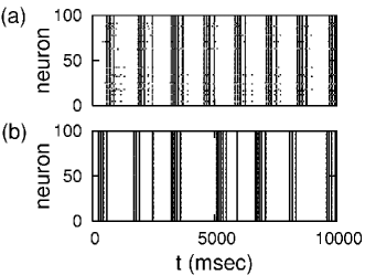
Figure 2: The results of numerical simulations of 100 MHH neurons with $g=0.02$ $\mbox{mS/cm}^{2}$ are plotted for (a) $T=11.9$˚C and (b) $T=12.1$˚C. Each dot represents spike timing in stationary state realized after $t=1.0\times 10^{7}$ msec.

When we assume weak gap junctions as in Fig. 1($g=0.02$ $\mbox{mS/cm}^{2}$), the condition for synchronization of MHH neurons is rather complicated. Periodic synchronous state is stable in some conditions and unstable in other conditions. We also see stable chaotic synchronous state in some values of temperature $T$. Around $T\sim 12$˚C we find unstable periodic synchronous state inside the periodic window (${\lambda^{\mbox{\tiny$\parallel$}}_{1}}=0$ and $0<{\lambda^{\mbox{\tiny$\perp$}}_{1}}$ at $T=11.9$˚C) while we find stable chaotic synchronous state outside the periodic window ($0<{\lambda^{\mbox{\tiny$\parallel$}}_{1}}$ and ${\lambda^{\mbox{\tiny$\perp$}}_{1}}<0$ at $T=12.1$˚C). Actually, the numerical simulations of 100 MHH neurons in Fig 2 show the good agreement with the results of our analysis. Around $T\sim 9.5$˚C, however, synchronous state is stable both inside and outside the periodic window. With weak gap junctions the condition for synchronization is so complicated that its intuitive explanation is difficult.

On the other hand, with strong gap junctions, synchronization of MHH neurons is stable over the wide range of temperature $T$. In Fig. 3, we plot the largest transversal Lyapunov exponent ${\lambda^{\mbox{\tiny$\perp$}}_{1}}$ as a function of $g$ for various values of temperature $T$. Eqs. (6) and (8) show that when parameter $g$ takes the zero value, transversal Lyapunov exponents ${\{{\lambda^{\mbox{\tiny$\parallel$}}_{l}}\}}$ take the same value as tangential Lyapunov exponents ${\{{\lambda^{\mbox{\tiny$\perp$}}_{l}}\}}$. Therefore, synchronous state in Fig. 3 is periodic for $T=6.5,\ 7,\mbox{ and }11.9$ (˚C) and chaotic for $T=7.5,\ 11,\mbox{ and }12.1$ (˚C). In these six temperature, the behavior of MHH neurons are quite different from one another. However, all ${\lambda^{\mbox{\tiny$\perp$}}_{1}}$ take negative values if we increase the strength of gap junctions beyond $g=0.05$. In all the temperature we investigate ($5{\char 23\relax\kern-3.00003pt\hbox{C}}<T<15{\char 23\relax\kern-3.00003pt\hbox{C}}$), we find a certain value of $g$ beyond which ${\lambda^{\mbox{\tiny$\perp$}}_{1}}$ always take a negative value. Irrespective of whether synchronous state is chaotic or periodic, strong gap junctions induce synchronization of neurons.

In summary, we have studied synchronous state of a large ensemble of modified Hodgkin-Huxley (MHH) neurons assuming gap junctions among neurons. For the general mean-field dynamics in Eq. (3), we have evaluated $N\times n$-dimensional deviation to define tangential Lyapunov exponents ${\{{\lambda^{\mbox{\tiny$\parallel$}}_{l}}\}}$ and transversal Lyapunov exponents ${\{{\lambda^{\mbox{\tiny$\perp$}}_{l}}\}}$. In Fig. 1(b), we have investigated characteristic of synchronous state of MHH neurons by the largest tangential Lyapunov exponent ${\lambda^{\mbox{\tiny$\parallel$}}_{1}}$. In Fig. 1(c), we have elucidated stability of this synchronization by the largest transversal Lyapunov exponent ${\lambda^{\mbox{\tiny$\perp$}}_{1}}$. With weak gap junctions $g=0.02$ $\mbox{mS/cm}^{2}$, stability of synchronization of MHH neurons shows rather complicated change with temperature as shown in Fig. 1(c). However, in Fig. 3 and so on, we have found that with strong gap junctions, synchronous state is stable over the wide range of temperature. The strong gap junctions induce synchronization both in periodic and chaotic neurons, and that implies a pivotal role of gap junctions in synchronization of the large number of neurons

It should be emphasized that the computational cost for Lyapunov exponents of four-dimensional MHH equations is not much higher than that of the three-dimensional Lorenz equations. Even when we assume dozens of ion channels in neuron dynamics, we would be able to calculate both Lyapunov exponents within the acceptable computation time. When synchronous state is periodic and interactions are infinitesimal ($g\ll 1$), one can use the phase reduction method. In the present system of MHH neurons, however, ${\lambda^{\mbox{\tiny$\perp$}}_{1}}$ in Fig. 3 fluctuates dramatically as $g$ increases, even if synchronous state is periodic. Since the synchronization property with finite $g$ is quite different from that with infinitesimal $g$, calculation of transversal Lyapunov exponents is indispensable in investigating the present system. In the real nervous system many types of neurons are interconnected with chemical synapses. Some authors model the dynamics of chemical synapse in the manner as $I_{i}=(g/N)\sum_{j}(v_{rev}-v_{i})s_{j}$, where constant $v_{rev}$ denotes reversal potential and $s_{j}$ obeys the dynamics $ds_{j}/dt=\alpha F(v_{j})(1-s_{j})-\beta s_{j}$ with the sigmoidal function $F(v)=1/(1+\exp[-(v-\theta_{syn})/2])$[22, 2, 5]. In this case, synchronous state ${{\bf x}}^{\ast}$ depends on $g$ since ${{\bf G}}({{\bf x}}^{\ast},{{\bf x}}^{\ast})$ does not vanish. Moreover, Jacobi matrices of ${{\bf G}}({{\bf x}}_{i},{{\bf x}}_{j})$ are not constant but depend on ${{\bf x}}_{i}$ and ${{\bf x}}_{j}$. Our analysis is applicable also to such complicated neural networks since their dynamics are written in the form of Eq. (3). Although pulse-coupled neural networks based on threshold-crossing spike timing cannot be written in the form of Eq. (3), we can employ the similar analysis by carrying out the decomposition of linear stability discussed in our previous study[8]. In that study, we have evaluated two types of Floquet matrices to show that periodic synchronous state of integrated-and-fire (IF) neurons are stable with only inhibitory chemical synapses. Interestingly, in the real nervous system, interneurons are found to be connected with inhibitory chemical synapses and gap junctions[20]. It turns out that networks of interneurons take the extremely ideal structure to induce synchronization of an ensemble of neurons. The present approach of stability analysis is applicable to a wide class of stability problems in neural networks. Retrieval state in associative memory neural networks of spiking neurons can be investigated by the similar stability analysis[21]. More complicated neural networks including pyramidal neurons and interneurons[23] would also be analyzed by the present approach.

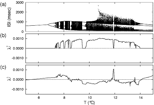
Figure 1: (a) The interspike intervals (ISIs) in stationary state of an isolated single MHH neuron are plotted as a function of temperature $T$. The ISI distribution of synchronous state of $N$ neurons ${{\bf x}}^{\ast}$ is the same as a isolated single neuron since the interaction term in Eq. (4) vanishes in the present system. (b) The largest tangential Lyapunov exponent ${\lambda^{\mbox{\tiny$\parallel$}}_{1}}$, which characterizes synchronous state ${{\bf x}}^{\ast}$ described in (a), is plotted. In the present system, ${\lambda^{\mbox{\tiny$\parallel$}}_{1}}$ is independent of $g$. (c) The largest transversal Lyapunov exponent ${\lambda^{\mbox{\tiny$\perp$}}_{1}}$ is plotted for $g=0.02$ $\mbox{mS/cm}^{2}$. When ${\lambda^{\mbox{\tiny$\perp$}}_{1}}$ takes a negative value, synchronization is stable. The sampling points are $T=5+0.025\times k\mbox{({\char 23\relax\kern-3.00003pt\hbox{C}})}\ (k=0,1,2,\ldots)$.

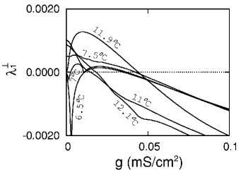
Figure 3: The largest transversal Lyapunov exponent ${\lambda^{\mbox{\tiny$\perp$}}_{1}}$ is plotted as a function of $g$ for various values of temperature $T$. The numbers in the figure indicate temperature $T$.

References

• [1] G. BuzsΓ‘ki, Z. HorvΓ‘th, R. Urioste, J. Hetke, and K.Β Wise, Science, 256, 1025 (1992).
• [2] X.JΒ Wang and J.Β Rinzel, J. Neurosci., 16, 6402 (1996).
• [3] D.Β Golomb and J.Β Rinzel, Phys. Rev. E, 48, 4810 (1993).
• [4] M.A.Β Whittington, R.D.Β Traub, and J.G.R.Β Jeffreys, Nature, 373, 612 (1995).
• [5] X.J.Β Wang and G.Β BuzΓ‘ki, J. Neurosci., 16, 6402 (1996).
• [6] C.C.Β Chow, J.A.Β White, J.Β Ritt, and N.Β Kopell, J. Comput. Neurosci., 5, 407 (1998).
• [7] P.H.EΒ Tiesinga and J.V.Β Jose, Network 11, 1 (2000).
• [8] M.Β Yoshioka, Phys. Rev. E, in press.
• [9] G.Β Ermentrout and N.Β Kopell, J. Math. Biol., 29, 195, (1991).
• [10] D.Β Hansel, G.Β Mato, and C.Β Meunier, Neural Comput., 7, 307 (1995).
• [11] Y.Β Kuramoto, Chemical oscillations, waves, and turbulence (Springer-Verlag 1984).
• [12] H.Β Fujisaka and T.Β Yamada, Prog. Theor. Phys. 69, 32 (1983).
• [13] K.Β Kaneko, Physica D, 77, 456 (1994).
• [14] Y.Β Maistrenko, T.Β Kapitaniak, and P.Β Szuminski, Phys. Rev. E, 54, 3285 (1996).
• [15] A.Β Pikovsky, O.Β Popovych, and Yu.Β Maistrenko, Phys. Rev. Lett., 87, 044102 (2001).
• [16] H.A.Β Braun, M.T.Β Huber, M.Β Dewald, K.Β SchΓ€fer, and K.Β Voigt, Int. J. Bifurcation Chaos Appl. Sci. Eng. 8, 881 (1998).
• [17] U.Β Feudel, A.Β Neiman, X.Β Pei, W.Β Wojtenek, H.Β Braun, M.Β Huber, and F.Β Moss, Chaos, 10, 231 (2000). According to this paper we assume the four-dimensional MMH equations of the form vΛ™=(βˆ’Ilβˆ’Idβˆ’Irβˆ’Is​dβˆ’Is​r)/c,Il=gl​(vβˆ’vl),Id=ρ​gd​αdβ€‹βˆžβ€‹(vβˆ’vd),Ξ±dβ€‹βˆž=(1+exp⁑[βˆ’sd​(vβˆ’v0​d)])βˆ’1,Ir=ρ​gr​αr​(vβˆ’vr),wΛ™1=Ξ±Λ™r=ϕ​(Ξ±rβ€‹βˆžβˆ’Ξ±r)/Ο„r,Ξ±rβ€‹βˆž=(1+exp⁑[βˆ’sr​(vβˆ’v0​r)])βˆ’1,Is​d=ρ​gs​d​αs​d​(vβˆ’vs​d),wΛ™2=Ξ±Λ™s​d=ϕ​(Ξ±s​dβ€‹βˆžβˆ’Ξ±s​d)/Ο„s​d,Ξ±s​dβ€‹βˆž=(1+exp⁑[βˆ’ss​d​(vβˆ’v0​s​d)])βˆ’1,Is​r=ρ​gs​r​αs​r​(vβˆ’vs​r),wΛ™3=Ξ±Λ™s​r=ϕ​(βˆ’Ξ·β€‹Is​rβˆ’ΞΈβ€‹Ξ±s​r)/Ο„s​rformulae-sequenceformulae-sequence˙𝑣subscript𝐼𝑙subscript𝐼𝑑subscriptπΌπ‘Ÿsubscript𝐼𝑠𝑑subscriptπΌπ‘ π‘Ÿπ‘formulae-sequencesubscript𝐼𝑙subscript𝑔𝑙𝑣subscript𝑣𝑙formulae-sequencesubscriptπΌπ‘‘πœŒsubscript𝑔𝑑subscript𝛼𝑑𝑣subscript𝑣𝑑formulae-sequencesubscript𝛼𝑑superscript1subscript𝑠𝑑𝑣subscript𝑣0𝑑1formulae-sequencesubscriptπΌπ‘ŸπœŒsubscriptπ‘”π‘Ÿsubscriptπ›Όπ‘Ÿπ‘£subscriptπ‘£π‘Ÿsubscript˙𝑀1subscriptΛ™π›Όπ‘Ÿitalic-Ο•subscriptπ›Όπ‘Ÿsubscriptπ›Όπ‘Ÿsubscriptπœπ‘Ÿformulae-sequencesubscriptπ›Όπ‘Ÿsuperscript1subscriptπ‘ π‘Ÿπ‘£subscript𝑣0π‘Ÿ1formulae-sequencesubscriptπΌπ‘ π‘‘πœŒsubscript𝑔𝑠𝑑subscript𝛼𝑠𝑑𝑣subscript𝑣𝑠𝑑subscript˙𝑀2subscript˙𝛼𝑠𝑑italic-Ο•subscript𝛼𝑠𝑑subscript𝛼𝑠𝑑subscriptπœπ‘ π‘‘formulae-sequencesubscript𝛼𝑠𝑑superscript1subscript𝑠𝑠𝑑𝑣subscript𝑣0𝑠𝑑1formulae-sequencesubscriptπΌπ‘ π‘ŸπœŒsubscriptπ‘”π‘ π‘Ÿsubscriptπ›Όπ‘ π‘Ÿπ‘£subscriptπ‘£π‘ π‘Ÿsubscript˙𝑀3subscriptΛ™π›Όπ‘ π‘Ÿitalic-Ο•πœ‚subscriptπΌπ‘ π‘Ÿπœƒsubscriptπ›Όπ‘ π‘Ÿsubscriptπœπ‘ π‘Ÿ\dot{v}=(-I_{l}-I_{d}-I_{r}-I_{sd}-I_{sr})/c,\ I_{l}=g_{l}(v-v_{l}),\ I_{d}=\rho g_{d}\alpha_{d\infty}(v-v_{d}),\ \alpha_{d\infty}=(1+\exp[-s_{d}(v-v_{0d})])^{-1},\ I_{r}=\rho g_{r}\alpha_{r}(v-v_{r}),\ \dot{w}_{1}=\dot{\alpha}_{r}=\phi(\alpha_{r\infty}-\alpha_{r})/\tau_{r},\ \alpha_{r\infty}=(1+\exp[-s_{r}(v-v_{0r})])^{-1},\ I_{sd}=\rho g_{sd}\alpha_{sd}(v-v_{sd}),\ \dot{w}_{2}=\dot{\alpha}_{sd}=\phi(\alpha_{sd\infty}-\alpha_{sd})/\tau_{sd},\ \alpha_{sd\infty}=(1+\exp[-s_{sd}(v-v_{0sd})])^{-1},\ I_{sr}=\rho g_{sr}\alpha_{sr}(v-v_{sr}),\ \dot{w}_{3}=\dot{\alpha}_{sr}=\phi(-\eta{}I_{sr}-\theta\alpha_{sr})/\tau_{sr} with temperature-dependent scaling factors $\rho=A_{1}^{(T-T_{0})/10}$ and $\phi=A_{2}^{(T-T_{0})/10}$. The parameters values are c=1,vl=βˆ’60,vd=vs​d=50,vr=vs​r=βˆ’90,gl=0.1,gd=1.5,gr=2.0,gs​d=0.25,gs​r=0.4,Ο„r=2.0,Ο„s​d=10,Ο„s​r=20,v0​d=βˆ’25,v0​r=βˆ’25,v0​s​d=βˆ’40,sd=0.25,sr=0.25,ss​d=0.09,Ξ·=0.012,ΞΈ=0.17,A1=1.3,A2=3.0,T0=25formulae-sequenceformulae-sequence𝑐1formulae-sequencesubscript𝑣𝑙60subscript𝑣𝑑subscript𝑣𝑠𝑑50subscriptπ‘£π‘Ÿsubscriptπ‘£π‘ π‘Ÿ90formulae-sequencesubscript𝑔𝑙0.1formulae-sequencesubscript𝑔𝑑1.5formulae-sequencesubscriptπ‘”π‘Ÿ2.0formulae-sequencesubscript𝑔𝑠𝑑0.25formulae-sequencesubscriptπ‘”π‘ π‘Ÿ0.4formulae-sequencesubscriptπœπ‘Ÿ2.0formulae-sequencesubscriptπœπ‘ π‘‘10formulae-sequencesubscriptπœπ‘ π‘Ÿ20formulae-sequencesubscript𝑣0𝑑25formulae-sequencesubscript𝑣0π‘Ÿ25formulae-sequencesubscript𝑣0𝑠𝑑40formulae-sequencesubscript𝑠𝑑0.25formulae-sequencesubscriptπ‘ π‘Ÿ0.25formulae-sequencesubscript𝑠𝑠𝑑0.09formulae-sequenceπœ‚0.012formulae-sequenceπœƒ0.17formulae-sequencesubscript𝐴11.3formulae-sequencesubscript𝐴23.0subscript𝑇025c=1,\ v_{l}=-60,\ v_{d}=v_{sd}=50,\ v_{r}=v_{sr}=-90,\ g_{l}=0.1,\ g_{d}=1.5,\ g_{r}=2.0,\ g_{sd}=0.25,\ g_{sr}=0.4,\ \tau_{r}=2.0,\ \tau_{sd}=10,\ \tau_{sr}=20,\ v_{0d}=-25,\ v_{0r}=-25,\ v_{0sd}=-40,\ s_{d}=0.25,\ s_{r}=0.25,\ s_{sd}=0.09,\ \eta=0.012,\ \theta=0.17,\ A_{1}=1.3,\ A_{2}=3.0,\ T_{0}=25.
• [18] I.Β Shimada and T.Β Nagashima, Prog. Theor. Phys. 61, 1605 (1979).
• [19] J. Milnor, Commun. Math. Phys. 99, 117 (1985).
• [20] M.Β Whittington and R.D.Β Traub, Trends Neurosci. 26, 676 (2003).
• [21] M.Β Yoshioka, Phys. Rev. E, 66, 061913 (2002).
• [22] D.H.Β Perkel, B.Β Mulloney, R.W.Β Budelli, Neurosci. 6, 823 (1981).
• [23] N.Β Kopell, G.B.Β Ermentrout, M.A.Β Whittington, and R.D.Β Traub, Proc. Natl. Acad. Sci. USA, 97, 1867 (2000).
Refer to caption
Figure 1: (a)Β The interspike intervals (ISIs) in stationary state of an isolated single MHH neuron are plotted as a function of temperatureΒ T𝑇T. The ISI distribution of synchronous state of N𝑁N neurons π±βˆ—superscriptπ±βˆ—{{\bf x}}^{\ast} is the same as a isolated single neuron since the interaction term in Eq.Β (4) vanishes in the present system. (b)Β The largest tangential Lyapunov exponentΒ Ξ»1βˆ₯subscriptsuperscriptπœ†parallel-to1{\lambda^{\mbox{\tiny$\parallel$}}_{1}}, which characterizes synchronous stateΒ π±βˆ—superscriptπ±βˆ—{{\bf x}}^{\ast} described in (a), is plotted. In the present system, Ξ»1βˆ₯subscriptsuperscriptπœ†parallel-to1{\lambda^{\mbox{\tiny$\parallel$}}_{1}} is independent of g𝑔g. (c)Β The largest transversal Lyapunov exponentΒ Ξ»1βŸ‚subscriptsuperscriptπœ†perpendicular-to1{\lambda^{\mbox{\tiny$\perp$}}_{1}} is plotted for g=0.02𝑔0.02g=0.02Β mS/cm2superscriptmS/cm2\mbox{mS/cm}^{2}. When Ξ»1βŸ‚subscriptsuperscriptπœ†perpendicular-to1{\lambda^{\mbox{\tiny$\perp$}}_{1}} takes a negative value, synchronization is stable. The sampling points are T=5+0.025Γ—k​(˚C)​(k=0,1,2,…)𝑇50.025π‘˜(˚C)π‘˜012…T=5+0.025\times k\mbox{({\char 23\relax\kern-3.00003pt\hbox{C}})}\ (k=0,1,2,\ldots).
Refer to caption