Bifurcation and Chaos in Coupled Ratchets
exhibiting Synchronized Dynamics

Abstract

The bifurcation and chaotic behaviour of unidirectionally coupled deterministic ratchets is studied as a function of the driving force amplitude ($a$) and frequency ($\omega$). A classification of the various types of bifurcations likely to be encountered in this system was done by examining the stability of the steady state in linear response as well as constructing a two-parameter phase diagram in the ($a-\omega$) plane. Numerical explorations revealed varieties of bifurcation sequences including quasiperiodic route to chaos. Besides, the familiar period-doubling and crises route to chaos exhibited by the one-dimensional ratchet were also found. In addition, the coupled ratchets display symmetry-breaking, saddle-nodes and bubbles of bifurcations. Chaotic behaviour is characterized by using the sensitivity to initial condition as well as the Lyapunov exponent spectrum; while a perusal of the phase space projected in the Poincar$\acute{e}$ cross-section confirms some of the striking features.

I Introduction

Coupled nonlinear systems possess a rich catalog of potentially useful dynamical behaviours including bifurcations, chaos and synchronization. They are central to the understanding of a wide variety of extended systems, e.g. a line of lattice oscillations or coupled plasma wave modes. A system of two oscillators could make a Hopf bifurcation to a second incommensurate frequency and follow a quasiperiodic route to chaos, in addition to period doubling and intermittency. Such routes to chaos was first observed by Ruelle and Takensruelle71 . Synchronization phenomena in coupled or driven nonlinear oscillators are of fundamental importance and have been extensively investigated both theoretically and experimentally in the context of many specific problems arising in laser dynamics, electronic circuits, secure communications and time series analysis zhang02 to mention a few. In a recent study, we observed phase synchronization in both unidirectionally vincent04 and bidirectionally vincent05 coupled deterministic ratchets that exhibits intermittent chaos. In vincent04 ; vincent05 , it was shown that the transition to the synchronous regime is characterized by an interior crises transition of the attractor in the phase space. Specifically, two analytic tests based on the Fujisaka and Yamada approach fujisaka83 ; yamada83 and that of Gauthier and Bienfang gauthier96 were employed to verify the stability of the synchronous state in reference vincent04 .

A clear understanding of coupled oscillator systems requires a study of the full spectrum of the operating regimes, including the nonsynchronous state ram00 . It has been reported that a group of interacting chaotic units that exhibits synchronization show some bifurcation cascades from disorder to partial and global order when varying the coupling strength zhang00 . Ding and Yang ding96 showed the existence of intermingled basins in coupled Duffing oscillators that exhibit synchronized chaos and conjectured that intermingled basins can be easily realized in the context of coupled oscillators and synchronized chaos. Extensive bifurcation analysis of two coupled periodically driven Duffing oscillators was done by Kozlowski et al. kozlowski95 . They showed that the global pattern of bifurcation curves in parameter space consists of repeated subpatterns similar to the superstructure observed for single, periodically driven, strictly dissipative oscillators. This study was recently extended to two coupled periodically driven double-well Duffing oscillators by Kenfack kenfack03 . The results revealed a striking departure from the single-well Duffing oscillators studied by Kozlowski et al kozlowski95 .

The literature is abundant with studies on coupled oscillator systems. At this point, we wish to refer the reader to some other recent studies that are related to the subject of this work  wirkus02 -raj99 . Motivated by this series of studies, we aim in this paper to explore some dynamical features hitherto not fully explored in the coupled ratchets with emphasies on the bifurcation structures preceeding the stable synchronous regime. The rest of the paper is organized as follows: Section 2 describes the equations of motion of the chaotic ratchet model and comment on the synchronization behaviour of the coupled system that is of interest in this study. In Section 3, we carry out a linear stability analysis of the system projected on the Poincar$\acute{e}$ map, while in Section 4, numerical results of bifurcations are presented. Chaotic behaviour is characterized in Section 5. The paper is concluded in Section 6.

II The Chaotic Ratchet Model

Let us consider the one-dimensional problem of a particle driven by a periodic time-dependent external force under the influence of an asymmetric potential of the ratchet type jung96 -mateos03b . The time average of the external force is zero. In the absence of stochastic noise, the dynamics is exclusively deterministic. The dimensionless equation of motion for a particle of unit mass moving in the ratchet potential $V(x)$ is given by

$${\ddot{x}+b\dot{x}+{\frac{dV(x)}{dx}}=a\cos(\omega_{D}t)}$$ (1)

Where time $t$ has been normalized in the unit of $\omega_{0}^{-1}$, the small resonant frequency of the system. Here, $a$ and $b$ are the forcing strength and the damping parameter, respectively. The dimensionless potential $V(x)$ is given by

$$V(x)=C-\frac{1}{4\pi^{2}\delta}[\sin 2\pi(x-x_{0})+0.25\sin 4\pi(x-x_{0})],$$ (2)

with constants $C\simeq 0.0173$ and $\delta\simeq 1.6$. The potential $V(x)$ is shifted by a value $x_{0}$ in order to place its minimum at the origin (see fig. 1). Notice that this asymmetric potential is periodic and has infinite potential wells.

The extended phase space in which the dynamic is taking place is three-dimensional, since we are dealing with an inhomogeneous differential equation with an explicit time dependence. We can rewrite equation (1) in autonomous form as a three dimensional dynamical system described by the coordinates:

$$\dot{x} = y,$$

$$\dot{y} = a\cos z-by-\frac{dV(x)}{dx},$$ (3)

$$\dot{z} = \omega_{D}.$$

Since equation (3) is nonlinear its solutions allow the possibility of periodic and chaotic orbits. For the purpose of this study, we consider a system of two identical unidirectionally coupled chaotic ratchets governed by:

$$\ddot{x}_{1}+b\dot{x}_{1}+\frac{dV(x_{1})}{dx_{1}} = a\cos(\omega t)$$ (4)

$$\ddot{x}_{2}+b\dot{x}_{2}+\frac{dV(x_{2})}{dx_{2}} = a\cos(\omega t)+c(\dot{x}_{1}-\dot{x}_{2})$$ (5)

Where $c$ is the coupling parameter. For $a=0.08092844$, $b=0.1$ and $\omega=0.67$, systems (4) and (5) exhibit stable phase synchronization when $0.89\leq c\leq 1.05$. The synchronization dynamics for $c=0.95$ shown in fig. 2, is determined by the behaviour of the following difference $x=x_{2}-x_{1}$. The phase difference is locked (full synchronization, $x=0$) after a short transient time. Prior to the phase locking event, the strange attractor undergoes a crises transition during which it is gradually destroyed and as the synchronization regime is approached, the attractor is again re-built vincent04 . To obtain approximate visualization of the attractors and their bifurcations we follow the procedure described in kozlowski95 ; kenfack03 . That is, we investigate the dynamics in the Poincar$\acute{e}$ sections denoted by $\sum$.

Figure 1: The ratchet potential ($C=0.0173,\delta=1.6$)

Figure 2: Synchronization dynamics showing the quantity $x=x_{2}-x_{1}$ as function of time, for $c=0.95$, $b=0.1$, $a=0.08092844$ and $\omega=0.67$

III Stability Analysis

To begin with, let us consider the basic mathematical principle underlying some expected topological structure of the coupled ratchets. Here we carry out a stability analysis of the coupled system (4) and (5) which can be written equivalently as

$$\frac{dV}{dt}=F(V,\psi)$$ (6)

Where $V(x_{1},v_{1},x_{2},v_{2},\omega)$ is an autonomous vector field and $\psi(a,b,c,\omega)$ is an element of the parameter space. Thus (4) and (5) become:

$$\dot{x}_{1} = v_{1}$$

$$\dot{v}_{1} = a\cos(\omega t)-bv_{1}+\frac{1}{4\pi\delta}{\bigg{[}}2\cos 2\pi(x_{1}-x_{0})+\cos 4\pi(x_{1}-x_{0}){\bigg{]}}$$

$$\dot{x}_{2} = v_{2}$$

$$\dot{v}_{2} = a\cos(\omega t)-bv_{2}+\frac{1}{4\pi\delta}{\bigg{[}}2\cos 2\pi(x_{2}-x_{0})+\cos 4\pi(x_{2}-x_{0}){\bigg{]}}+c(v_{1}-v_{2})$$ (7)

The system described by (7) generates a flow $\phi=\{\phi^{T}\}$ on the phase space $\Re^{4}\times S^{1}$ such that a global map

$$P:\sum \to \sum$$

$$V_{p}(x_{1},v_{1},x_{2},v_{2}) \to P(V_{p})=\{\phi^{T}\}|_{\sum(x_{1},v_{1},x_{2},v_{2},\theta_{0})}$$

exist, with $\theta_{0}$ being a constant determining the location of the Poincar$\acute{e}$ cross-section defined by $\sum=\{(x_{1},v_{1},x_{2},v_{2},\theta)\ \epsilon\ \Re^{4}\times S^{1}|\theta=\theta_{0}\}$ on which coordinates of attractors $(x_{1},v_{1},x_{2},v_{2})$ are expressed. By employing the linear perturbation method which consists of considering the solution $X(x_{1},v_{1},x_{2},v_{2})$ as a superposition of a very small perturbation $Y(\delta x_{1},\delta v_{1},\delta x_{2},\delta v_{2})$ to the steady state $V_{0}(x_{10},v_{10},x_{20},v_{20})$, that is $X=V_{0}+Y$, we obtain the matrix variational equation

$$\dot{Y}=DG(V_{0})Y$$ (8)

where $DG(V_{0})$ is the $4\times 4$ Jacobian matrix

$$DG(V_{0})=\left(\begin{array}[]{cccc}0&1&0&0\\ \alpha&-b&0&0\\ 0&0&0&1\\ 0&c&\beta&-(b+c)\end{array}\right)$$ (9)

describing the vector field along the solution $Y$ and $V_{0}$ being an equilibrium point or steady state with $\alpha=-\frac{2}{\delta}(1+3\pi(x_{10}-x_{0}));\beta=-\frac{2}{\delta}(1+3\pi(x_{20}-x_{0}))$. The solution of equation (8) after one period $T$ of the oscillations in the linearized Poincar$\acute{e}$ map is given by

$$Y(T)=Y(0)\exp(DG(V_{0})T)$$ (10)

where $DG(V_{0})$ represents the time-independent stability matrix of a periodic orbit connecting arbitrary infinitesimal variations in the initial conditions $Y_{0}=Y(0)$ with corresponding change $Y(T)$ after one period $T$. The real parts of the roots of the characteristic equation $det(DG(V_{0})-I\lambda)=0$, given by

$$\lambda^{4}+A_{3}\lambda^{3}+A_{2}\lambda^{2}+A_{1}\lambda+A_{0}=0$$ (11)

determines the stability of the periodic motion, with $A_{3}=2b+c$, $A_{2}=b(b+c)-(\alpha+\beta)$, $A_{1}=-b(\beta+\alpha)+\alpha c$ and $A_{0}=\alpha\beta$. Here $\lambda=(\lambda_{j})$ represent the eigenvalues of $DG(V_{0})$. If one assumes $x_{0}\approx x_{10}\approx x_{20}$, as in our numerical experiment, then $\alpha=\beta=-\frac{2}{\delta}$. In general, complex eigenvalues occur in complex conjugate pairs. Let us consider $\alpha_{k}$, $\beta_{k}$ as the real and the imaginary parts of $\lambda_{k}$, respectively ($\lambda_{k}=\alpha_{k}+i\beta_{k}$). If $\lambda_{k}$ is real, the eigenvalues are simply the rate of contraction ($\alpha_{k}<0$) or expansion ($\alpha_{k}>0$) near the steady state. If $\lambda_{k}$ is complex, its real part $\alpha_{k}$ gives the rate of contraction ($\alpha_{k}<0$) or expansion ($\alpha_{k}>0$) of the spiral while its imaginary part $\beta_{k}$ contributes for the frequency rotation. The eigenvalues of the linearized Poincar$\acute{e}$ map may thus be written as :

$$\sigma_{k}=\exp(\alpha_{k}T)\left(\cos(\beta_{k}T)+i\sin(\beta_{k}T)\right)$$ (12)

It turns out from equation (12) that if $\alpha_{k}<0$ for all $\lambda_{k}$, then all sufficiently small perturbations tend torward zero as $t\to\infty$ and the steady state (node (n), saddle-node (sn), spiral (sp)) is stable. If $\alpha_{k}>0$ for all $\lambda_{k}$, then any small perturbation grows with time and the steady state (n, sn, sp) is unstable. In addition if there exist $m$ and $l$ such that $\alpha_{m}<0$ and $\alpha_{l}>0$, the equilibrium state is unstable and is called a saddle. Having recourse to the above analysis it follows that saddle-node, sn ($\lambda_{k}=+1$), period-doubling, pd ($\lambda_{k}=-1$), Hopf ($\beta_{k}\neq 0$, with $\alpha_{k}<0$) and symmetry-breaking (sb) bifurcations are expected to occur in the coupled ratchets. Similar bifurcational scenario have been found in periodically driven coupled single kozlowski95 and double kenfack03 well Duffing oscillators.

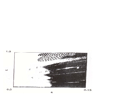
Figure 3: Two parameter phase diagram in the ($a-\omega$) plane. Regions of period-2 ($\circ$), period-3 ($\bullet$), period-4 ($+$), chaos (black) and non-attraction (white) can be identified.

IV Bifurcation Diagrams

In order to investigate the dependence of the system on a single control parameter (in this case, the amplitude $a$ of the driving function), several bifurcation diagrams have been computed, some of which have been chosen to illustrate the general structure of the system. Each bifurcation diagram shows the projection of the attractors in the Poincar$\acute{e}$ section onto the $x_{2}$ or the $v_{2}$ coordinates versus the control parameter. We employ this technique in our numerical exploration using the period $T=2\pi/\omega$ of oscillation as the stroboscopic time; with the standard 4th order Runge Kutta algorithm.

In what follows, we consider the bifurcational precedencies of formation of the stable synchronized chaos in the synchronization regime i.e in the neighbourhood of $0.89\leq c\leq 1.05$. We begin with a general overview of the behaviour of the two coupled systems by displaying regions of existence of different periodic and chaotic orbits in a two parameter phase diagram which is plotted in ($a-\omega$) plane at fixed values of $b=0.1$ and $c=0.5$ (fig. 3). We obtained the parameter phase diagram using the software dynamics nusse98 . Different regions of periodic orbits of period-2 ($\circ$), period-3 ($\bullet$), period-4 ($+$) as well as chaotic orbits (black region) are clearly visible. Besides the periodic and the chaotic orbits, there also exist non-attracting points (white region) for which the orbits diverge.

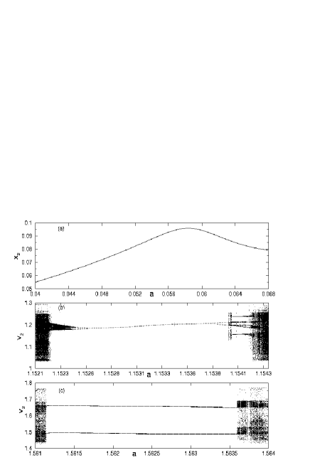
Figure 4: Bifurcation diagrams for the driving frequency $\omega=0.3$, showing (a) a resonance near $a=0.0559$, (b) a period-1 and (c) a large windows of period-2, both sandwiched in the chaotic regions.

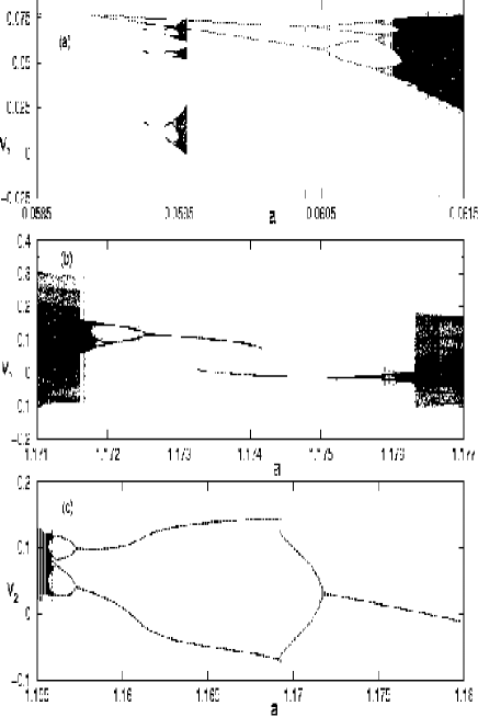
Figure 5: Bifurcation diagrams for the driving frequencies (a) $\omega=0.4$, (b) $\omega=0.5$ and (c) $\omega=0.75$ showing clearly the occurence of sn, sb, reversed pd and pd route to chaos.

In fig. 4 we show bifurcation diagrams for a comparatively small driving frequency of $\omega=0.3$. Different bifurcation sequences occur as the driving amplitude $a$ is varied. For instance in fig. 4(a), there is a resonance near $a=0.0559$ while a period-1 attractor emerges in fig. 4(b) from chaos, through a reversed period-doubling (pd) and subsequently follows the familiar pd route to chaos. For much larger amplitude of the driving force, a large period-2 is suddenly created at around $a=1.5612$ from a chaotic region, (see fig. 4(c)). This period-2 attractor is finally annihilated in a crisis event around $a=1.5638$ leading to a sudden chaotic state (transcient chaotic state). After this chaotic state we find bubbles of bifurcation dominating periodic windows (further, see fig. 7(a) as a prototype). When the driving frequency $\omega$ is increased, saddle-node (sn), symmetry breaking (sb) bifurcations, quasiperiodicity as well as period-doubling (pd) cascade predominate. For instance, fig. 5(a) shows the occurence of sn in the vicinity of $a=0.05925$ and a pd cascade, at around $a=0.06075$, leading to chaos for $\omega=0.4$. Moreover $sb$ and sn resulting from a reversed pd are clearly visible in fig. 5, (b) for $\omega=0.5$ and (c) for $\omega=0.75$. Similar routes identified in this transport model have also been found in the coupled Duffing model kozlowski95 ; kenfack03 .

To complete our bifurcation study, we proceed to investigate large values of the driving frequency ($\omega>\omega_{c}=0.8$) and different ranges of $a$. Here we find that the majority of the earlier observed bifurcation scenario are also repeated except that for large $a$, typically greater than the critical value $a_{c}=1.17$, periodic attractors dominate. Fingerprints of such behaviour can readily be observed in fig. 5(c) for $\omega=0.75$, where a period-1 attractor is created via a sb bifurcation.

V Characterizing Chaos

The best-known characteristic of a chaotic system is unpredictability, resulting from sensitivity to initial conditions (SIC). The slightest deviation from a given set of initial conditions yields a completely different output. In fig. 6, two typical chaotic trajectories originated from two slightly different set of initial conditions ($x_{2}=0.0$ for A and $x_{2}=0.01$ for B) are displayed. The parameters have been selected from the chaotic region of the phase diagram of fig. 3 with the driving amplitude kept fixed $a=0.08092844$. Although both trajectories initially evolve together, after several time steps the state variables become essentially independent. This is a clear manifestation of the SIC, as witness of chaos.

Though SIC has come to be the hallmark of chaos, it is not unique to the chaotic regime. For example, a similar behaviour can be observed in the intermittency transition regime where the time series is nearly periodic. Thus, to better validate the results obtained above, it is necessary to investigate the dynamics of the ratchets in a more concrete space - the poincare cross-sections. Analysis of the dynamics in such space may help to eventually uncover the hidden structure in the behaviour of the coupled ratchets. In the poincare cross-section, all trajectories for a given set of control parameters converge to a single object (the attractor) in spite of SIC. The convergence to an attractor is guaranteed even if the control parameters are slightly varied.

The set of Lyapunov exponents $\lambda_{k}$ provides an intuitively appealing and yet a very powerful measure of SIC and dissipation, both of which are required for a chaotic system. All $\lambda_{k}$ originates from linear stabilty analysis. In this approximation, all solutions are of the form $\exp(\lambda_{k}t)$, $k=1,2,...M$. The maximum Lyapunov exponent $\lambda_{max}$ is defined as:

$$\lambda_{max}=\lim_{\tau\to+\infty}\frac{1}{\tau}\ln(||L(\tau)||),$$ (13)

where $||L(\tau)||=(\delta x_{1}^{2}+\delta v_{1}^{2}+\delta x_{2}^{2}+\delta v_{2}^{2})^{\frac{1}{2}}$ is obtained in the Poincar$\acute{e}$ cross-section by solving numerically the variational equation (8) simultaneously with the systems (4) and (5). A positive Lyapunov exponent is a signature of chaos while zero and negative values of the exponent is an indication of a marginally stable or quasiperiodic orbit and periodic orbit, respectively. In fig. 7(b), a spectrum of the $\lambda_{max}$, corresponding to the bifurcation diagram of fig. 7(a) obtained for $\omega=0.3$, is displayed. Regions of chaotic and periodic solutions are well characterized. Various bifurcation scenario can be found including sn, sb, quasiperiodic region and pd cascade leading to chaos. Interestingly, bubbles of bifurcation beneath the chaotic region at $a=1.5630$, which by eyes test seems to be chaotic as well is not the case indeed. The Lyapunov spectrum shows that this regime is just a purely quasiperiodic one which yields precisely a period-4 attractor through a reversed pd.

Figure 6: Typical chaotic trajectories of particle for two slightly different sets of initial conditions ($x_{1}=v_{1}=x_{2}=v_{2}=0.0$ for A and $x_{1}=v_{1}=v_{2}=0.0,x_{2}=0.01$ for B). This is a clear manifestation of SIC.

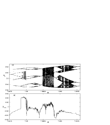
Figure 7: (a) Bifurcation diagram for $\omega=0.3$ and (b) the corresponding Lyapunov spectrum in the Poincare map.

Finally in fig. 8, we visualise the attractors in the Poincar$\acute{e}$ cross-sections for a fixed valued of the driving force $a=0.080928844$ and for several values of the driving frequency $\omega$ taken from fig. 3. We find that as $\omega$ is increased, the chaotic attractor shrinks (See fig. 8, (a) for $\omega=0.4$, (b) for $\omega=0.5$ and (c) for $\omega=0.75$). As a consequence, the attractor size gets enlarged as $\omega$ decreases. Essentially, this phenomenon has been attributed to the collision of the attractor with a periodic orbit in the exterior of its basin and is thus referred to as boundary crises ott02 . For larger $\omega$ values, quasiperiodic and periodic attractors were found to dominate. As an example, fig.8(d) shows a quasiperiodic attractor of period-2 for $\omega=\omega_{c}=0.8$.

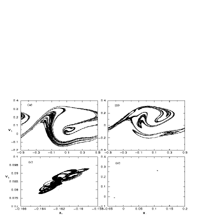
Figure 8: Typical attractors for parameters taken from fig.3, with a fixed value of the driving amplitude $a=0.08092844$. Shown are chaotic attractors (a) for $\omega=0.4$, (b) for $\omega=0.5$, (c) for $\omega=0.75$ and (d) a quasiperiodic attractor of period-2 for $\omega=0.8$.

VI Conclusions

In summary, we have investigated the dynamics of unidirectionally coupled deterministic ratchets and have shown varieties of bifurcation sequences including quasiperiodic route to chaos. Using the standard method of linear stability analysis, we have examined the stability of the steady state solution of the system leading to different types of bifurcations likely to occur in the neigbourhood of the synchronized region. For a given driving frequency, the bifurcations depend strongly on the values of the driving amplitude $a$ and are generally complicated. Besides quasiperiodicity, the familiar period-doubling and crisis route to chaos were also observed. In addition, the coupled ratchets exhibits symmetry-breaking bifurcations, resonance, saddle-node and bubbles of bifurcations. Using Lyapunov exponent spectrum as well as sensitivity to initial conditions, we characterized chaos in this system. A perusal of the Poincar$\acute{e}$ cross-sections revealed boundary crises in which the size of chaotic attractor is suddenly enlarged as the driving frequency is gradually decreased for a fixed driving amplitude. Although this system presents a very chaotic structure, it remains nevertheless ordered as the driving frequency becomes large, thereby providing critical parameters for a chaotic transport of particles. This makes the present study essentially interesting for technological applications.

VII acknowledgements

UEV gratefully acknowledges Prof. Jose L. Meteos of the Instituto de Fisica, Universidad Nacional Autonoma de Mexico, Mexico, for supplying relevant literatures and very useful discussions. AK gratefully acknowledges the financial support of the Alexander von Humboldt (AvH) Foundation/Bonn-Germany, under the grant of Research fellowship no IV.4-KAM 1068533 STP. We are grateful to Dr. E. Arevalo for a careful reading of the manuscript.

References

- (1) D. Ruelle and F. Takens, Commun. Math. Phys. 20 (1971) 167
- (2) Z. Zhang, X. Wag and M. C. Cross, Phys. Rev. E 65 (2002) 056211
- (3) U. E. Vincent, A. N. Njah, O. Akinlade and A. R. T. Solarin, Chaos 14, (2004) 1018.
- (4) U. E. Vincent, A. N. Njah, O. Akinlade and A. R. T. Solarin, ’Phase synchronization in coupled chaotic ratchets - Unpublished.
- (5) H. Fujisaka and T. Yamada, Prog. Theor. Phys. 69 (1983) 32
- (6) T. Yamada and H. Fujisaka, Prog. Theor. Phys. 70 (1983) 1240.
- (7) D. J. Gauthier and J. C. Bienfang, Phys. Rev. Lett. 77 (1996) 1752.
- (8) R.J. Ram, R. Sporer, A. R. Blank and R. A. York, IEEE Trans. Microwave Theor. Techn. 48 (2000) 1909.
- (9) G. H. Y. Zhang, H. A. Cerdeira, and S. Chen, Phys. Rev. Lett. 85 (2000) 3380.
- (10) M. Ding and W. Yang, Phys. Rev. E 54 (1996) 2189.
- (11) J. Kozlowski, U. Parlitz and W. Lanterborn, Phys. Rev. E 51 (1995) 1861.
- (12) A. Kenfack, Chaos, Sol. and Fract. 15 (2003) 205.
- (13) S. Wirkus, R. Rand, Nonl. Dynamics 30 (2002) 205.
- (14) P. Woafo, J. C. Chedjou and H. B. Fotsin, Phys. Rev. E 54 (1996) 5929.
- (15) G. L. Baker, J. A. Blackburn, H. J. T. Smith, Phys. Rev. Lett. 81 (1998) 554.
- (16) Y. Chen, G. Rangarjan and M. Ding, Phys. Rev.E 67 (2003) 026209.
- (17) T. Hikihara, K. Torii and Y. Ueda, Phys. Lett. A. 281 (2001) 155.
- (18) H. J. T. Smith, J. A. Blackburn and G. L. Baker, Int. J. Bifurc. Chaos 13 (2003) 7.
- (19) A. F. Va Kakis and R. Rand, Int. J. of Nonlinear Mechanics 39 (2004) 1079.
- (20) S. P. Raj. S. Rajaskar and K. Murali, Phys. Lett. A 264 (1999) 283.
- (21) P. Jung, J. G. Kissner, and P. Hanggi, Phys. Rev. Lett. 76 (1996) 3436.
- (22) J. L. Meteos, Phys. Rev. Lett. 84 (2000) 258.
- (23) J. L. Meteos, Physica D 168 (2002) 205.
- (24) J. L. Meteos, Physica A 325 (2003) 92.
- (25) J. L. Meteos, Comm. Nonl. Sci. Num. Sim. 8 (2003) 253.
- (26) H. E. Nusse and J. A. Yorke ,Dynamics: Numerical Exploration: Springer-Verlag, 1998.
- (27) E. Ott, Chaos in Nonlinear Dynamical Systems (Cambridge University Press, Cambridge, 2002).