Spectral Form Factor for Chaotic Dynamics
in a Weak Magnetic Field

Abstract

Using semiclassical periodic orbit theory for a chaotic system in a weak magnetic field, we obtain the form factor predicted by Pandey and Mehta’s two matrix model up to the third order. The third order contribution has a peculiar term which exists only in the intermediate crossover domain between the GOE (Gaussian Orthogonal Ensemble) and the GUE (Gaussian Unitary Ensemble) universality classes. The exact expression is obtained by taking account of the contribution from encounter regions where orbit loops are connected.

^∗ Department of Physics, Graduate School of Science, University of Tokyo, Hongo 7-3-1, Bunkyo-ku, Tokyo 113-0033, Japan

^† Graduate School of Mathematics, Nagoya University, Chikusa-ku,
Nagoya 464-8602, Japan

PACS: 05.45.+b; 05.40.+j

KEYWORDS: quantum chaos; periodic orbit theory; random matrices

1 Introduction

Universal level statistics of classically chaotic systems in agreement with the RMT (Random Matrix Theory) prediction has been intensively studied since it was conjectured two decades ago[1].

Berry[2] first evaluated the first order term of the spectral form factor using the semiclassical periodic orbit theory[3]. His method is called the diagonal approximation. It is applicable to both of the GOE (Gaussian Orthogonal Ensemble) and GUE (Gaussian Unitary Ensemble) universality classes. In the absence of time reversal invariance, the first order term is evaluated as a sum over the periodic orbits and agrees with the prediction derived from the GUE of random matrices. If the system is time reversal invariant, we additionally need to sum up over the pairs of the periodic orbits mutually time reverse. The result is also in agreement with the RMT prediction derived from the GOE.

Recently Sieber and Richter (SR) showed that a family of orbit pairs with an encounter gave the first correction to the diagonal approximation [4]. Their idea clarifies what corresponds to the order of each term in the context of the periodic orbit theory. Heusler et al. [5] further generalized SR’s idea by using a combinatorial analysis and Müller et al.[6, 7] obtained the full expansion which yields the RMT form factor.

In this paper, we investigate the form factor of chaotic systems in a weak magnetic field, extending the method of Ref.[5]. Our aim is to reproduce the universal level statistics in the crossover domain between the GOE and GUE universality classes. The corresponding RMT formula is derived from Pandey and Mehta’s two matrix model[8]. This formula interpolates the form factors of GOE and GUE, which correspond to chaotic systems without and with a magnetic field, respectively. Using a quantum graph, the authors previously obtained the second order term by employing Sieber and Richter’s periodic orbit pairs and showed that it agreed with the RMT prediction[9]. Here we consider the third order term of the form factor and clarify a mechanism to yield the RMT expression. We show that the RMT expression is obtained by taking account of the interference of the gauge potential in the encounters of periodic orbits.

Let us explicitly present the RMT prediction of the form factor. It is derived from Pandey and Mehta’s two matrix model, as explained in[9]. For small $\tau(0\leq\tau\leq{1\over 2})$, the RMT form factor $K_{\rm RM}(\tau)$ with a parameter $\mu$ is written as

$$K_{\rm RM}(\tau) = \tau+{1\over 2}\int_{1-2\tau}^{1}dk\,{k\over k+2\tau}e^{-\mu(k+\tau)}$$ (1)

$$= \tau+\tau e^{-\mu}-2\tau^{2}e^{-\mu}+\tau^{3}\left({\mu^{2}\over 6}e^{-\mu}+2e^{-\mu}\right)+\cdots.$$

The GOE and GUE limits correspond to $\mu\to 0$ and $\mu\to\infty$, respectively. Up to the second order of $\tau$, each term is a monotonic function of the parameter $\mu$. However, the third order term in (1) includes a peculiar nonmonotonic term $\tau^{3}{\mu^{2}\over 6}e^{-\mu}$, which vanishes in both of the GOE and GUE limits. Such terms generally appear in higher order contributions. We can thus expect that a semiclassical analysis of the third order term will offer a basis to reproduce the full expansion of $K_{\rm RM}(\tau)$.

2 Chaotic System in a Magnetic Field and Periodic Orbit Theory

We consider a quantum system in a magnetic field and assume that the corresponding classical dynamics is chaotic. In the semiclassical limit $\hbar\rightarrow 0$, the form factor of such a system can be formally written in terms of the classical periodic orbits[3];

$$K_{\rm po}(\tau)=\left\langle\sum_{\gamma,\gamma^{\prime}}A_{\gamma}A_{\gamma^{\prime}}^{\ast}e^{i(S_{\gamma}+\theta_{\gamma})/\hbar}e^{-i(S_{\gamma^{\prime}}+\theta_{\gamma^{\prime}})/\hbar}\delta\left(\tau-{T_{\gamma}+T_{\gamma^{\prime}}\over 2T_{\rm H}}\right)\right\rangle,$$ (2)

where $S_{\gamma}$, $T_{\gamma}$ and $A_{\gamma}$ are the action without gauge potential (including the Maslov phase), period and dimensionless stability amplitude of the periodic orbit $\gamma$. The phase $\theta_{\gamma}$ is an effect of the gauge potential in the action along the orbit $\gamma$, i.e., $\theta_{\gamma}=\int_{\gamma}d{\bf x}_{\gamma}\cdot{\bf a}({\bf x}_{\gamma})=\int_{\gamma}dt\,d{\bf x}_{\gamma}/dt\cdot{\bf a}({\bf x}_{\gamma})$, using the gauge potential ${\bf a}({\bf x}_{\gamma})$ at the position ${\bf x}_{\gamma}$. The angular bracket stands for an average over the mean energy $(E+E^{\prime})/2$ and over a time interval much smaller than the Heisenberg time $T_{\rm H}$. Since the classical dynamics is chaotic, each periodic orbit shows a diffusive behavior[10, 11]; successive changes of the velocity can be regarded as independent events. Hence, if the time $T$ elapsed on an orbit $\gamma$ is sufficiently large, we assume that the term $g_{\gamma}(t)\equiv d{\bf x}_{\gamma}/dt\cdot{\bf a}({\bf x}_{\gamma})$ can be replaced by the Gaussian white noise satisfying the correlation $\langle\langle g_{\gamma}(t)g_{\gamma}(t^{\prime})\rangle\rangle=2D\delta(t-t^{\prime})$. Here a Gaussian average $\langle\langle\cdots\rangle\rangle$ is computed as a functional integral

$$\langle\langle\ F[g_{\gamma}]\ \rangle\rangle=\frac{\displaystyle\int{\cal D}g_{\gamma}\ {\rm exp}\left[-\frac{1}{4D}\int_{0}^{T}dt(g_{\gamma}(t))^{2}\right]F[g_{\gamma}]}{\displaystyle\int{\cal D}g_{\gamma}\ {\rm exp}\left[-\frac{1}{4D}\int_{0}^{T}dt(g_{\gamma}(t))^{2}\right]}.$$ (3)

Incorporating such a Gaussian average, we obtain a formula

$$K_{\rm po}(\tau)=\left\langle\sum_{\gamma,\gamma^{\prime}}A_{\gamma}A_{\gamma^{\prime}}^{\ast}e^{i(S_{\gamma}-S_{\gamma^{\prime}})/\hbar}\langle\langle e^{i(\theta_{\gamma}-\theta_{\gamma^{\prime}})/\hbar}\rangle\rangle\delta\left(\tau-{T_{\gamma}+T_{\gamma^{\prime}}\over 2T_{\rm H}}\right)\right\rangle.$$ (4)

We start from Berry’s diagonal approximation, which yields the first order term[2]. This term is obtained from two types of periodic orbit pairs $({\gamma,\gamma})$ and $({\gamma,\overline{\gamma}})$. Here a periodic orbit $\overline{\gamma}$ is the time reverse of $\gamma$. For the pairs of identical orbits $({\gamma,\gamma})$, the dependence on the gauge potential is canceled, so that the result does not depend on the magnetic field. The estimate for the form factor is given by the Hannay and Ozorio de Almeida (HOdA)’s sum rule[12];

$$\sum_{\gamma}\left|A_{\gamma}\right|^{2}\delta\left(\tau-{T_{\gamma}\over T_{H}}\right)=\tau.$$ (5)

For the pairs of mutually time reverse orbits $({\gamma,\overline{\gamma}})$, on the other hand, the result depends on the magnetic field. It is estimated as

$$\sum_{\gamma}\left|A_{\gamma}\right|^{2}\delta\left(\tau-{T_{\gamma}\over T_{H}}\right)\langle\langle e^{i(\theta_{\gamma}-\theta_{\overline{\gamma}})/\hbar}\rangle\rangle=\tau\langle\langle e^{2i\theta_{\gamma}/\hbar}\rangle\rangle=\tau e^{-bT},$$ (6)

where the last equality results from the Gaussian average (3). Here $T$ is the period $T(=\tau T_{H})$ and $b$ is defined in terms of the diffusion constant $D$ as $b=4D/\hbar^{2}$, which depends on the magnetic field. Putting the above results together, we reproduce the first order term of the form factor [13] as

$$K_{\rm po}^{(1)} = \tau+\tau e^{-bT},$$ (7)

which reproduces the first two terms of the RMT prediction (1). The RMT parameter $\mu$ is identified with $bT$.

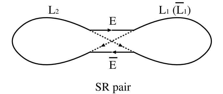
Figure 1: The Sieber-Richter (SR) pair of periodic orbits

We next consider the second order term. As shown by Sieber and Richter (SR) [4], a family of orbit pairs with one encounter plays a crucial role[9, 10]. We can symbolically write SR pairs as $\gamma=EL_{1}\overline{E}L_{2}$ and $\gamma^{\prime}=E\overline{L}_{1}\overline{E}L_{2}$ (see Figure 1). Here $E$ and its almost time reverse $\overline{E}$ are the orbit segments in the encounter where two loops are connected. The loops are denoted as $L_{1}$ and $L_{2}$, respectively, and $\overline{L}_{1}$ is the time reverse of $L_{1}$. Let us see the behavior of the periodic orbits $\gamma$ and $\gamma^{\prime}$ in the encounter region. The directions of encounter orbits are depicted as        for $\gamma$ and        for $\gamma^{\prime}$. For a system with two degrees of freedom, it is convenient to use the Poincaré section ${\cal P}$ in the phase space [5]. The orbit $\gamma$ pierces through $\cal P$ at two phase space points denoted by vectors $x_{a}$ and $x_{b}$. Let us express ${\cal T}x_{b}-x_{a}$ (${\cal T}$ is the time reversal operator) in terms of the pairwise normalized vectors $\hat{e}_{s}$ and $\hat{e}_{u}$ as ${\cal T}x_{b}-x_{a}=u\hat{e}_{u}+s\hat{e}_{s}$. To demand that the orbits in the encounter are mutually close, we introduce a bound $c$ and assume that $|u|,|s|<c$. Then the partner orbit $\gamma^{\prime}$ (or the time reverse of $\gamma^{\prime}$) pierces at $x_{a}^{p}=x_{a}+u\hat{e}_{u}$ and at $x_{b}^{p}={\cal T}(x_{a}+s\hat{e}_{s})$. We can consequently estimate the duration $t_{\rm enc}$ of the encounter and the action difference $\Delta S$ for the two orbits as

$$t_{\rm enc}={1\over\lambda}\ln{c^{2}\over|us|}\qquad{\rm and}\qquad\Delta S=us,$$ (8)

where $\lambda$ is the Liapunov exponent.

We need to estimate the number of encounters in one periodic orbit of a period $T$. This can be computed as

$$\int_{-c}^{c}duds\int_{0}^{T-2t_{\rm enc}}dT_{1}{T\over{\cal N}t_{\rm enc}\Omega},$$ (9)

where $\Omega^{-1}(={1\over 2\pi\hbar T_{H}})$ is the ergodic return probability per a unit action. The factor $T\int_{0}^{T-2t_{\rm enc}}{\rm d}T_{1}$ indicates that one of the two piercings occurs in the time interval $[0,T]$ and that the time $T_{1}$ elapsed on the loop $L_{1}$ or $\overline{L}_{1}$ lies in $[0,T-2t_{\rm enc}]$. The combinatorial factor ${\cal N}=2$ is necessary to avoid a double counting due to the equivalence of $E$ and $\overline{E}$ in $\gamma$.

Let us now evaluate the contribution of the gauge potential to the second order term. The Gaussian average (3) yields a factor $e^{-bT_{1}}$ as a contribution from the the pair of the loops $L_{1}$ and $\overline{L}_{1}$. In the region of the encounter, the gauge potential destructively interferes with itself and yields no contribution. That is, since mutually almost time reversed orbits are combined in the encounter, a product of the phase factors $e^{i\theta_{\gamma}}$ and $e^{-i\theta_{\gamma^{\prime}}}$ gives a factor $1$. Incorporating the factor $2$ due to the time reversal of the orbit $\gamma^{\prime}$, we obtain the second order term as

$$K_{\rm po}^{(2)}(\tau) = 2\sum_{\gamma}\left|A_{\gamma}\right|^{2}\delta\left(\tau-{T_{\gamma}\over T_{H}}\right)\int_{-c}^{c}duds\int_{0}^{T-2t_{\rm enc}}dT_{1}{T\over{\cal N}t_{\rm enc}\Omega}e^{-bT_{1}}e^{ius/\hbar}$$ (10)

$$\rightarrow -2\tau^{2}e^{-bT},$$

again in agreement with (1). Here we calculated only the term independent of $t_{\rm enc}$, as the other terms vanish due to appearances of extra factors $\hbar$ or rapid oscillations[7].

3 Third Order Term

We now calculate the third order contribution, following the recipe explained in previous section. We will find that the calculation is somewhat different from the second order term because the interference of the gauge potential in the encounter regions gives a significant contribution. For the periodic orbit pairs which contribute to the third order term, Heusler et al.[5] introduced several notations (aas, api, ppi, ac and pc). In order to take account of the time reversal of the orbit $\gamma^{\prime}$, we modify their notations by putting suffixes (-a and -b) as drawn in Figures 2 and 3.

Let us first consider a general orbit pair $\alpha$ with $L$ loops and $V$ encounters. Extending the result (9) for the second order term, we can compute the number of encounters in one periodic orbit of a period $T$ as

$$\int d{\bf u}d{\bf s}\int_{0}^{T-t_{\alpha}}dT_{1}\int_{0}^{T-t_{\alpha}-T_{1}}dT_{2}\cdots\int_{0}^{T-t_{\alpha}-T_{1}-T_{2}-\cdots-T_{L-2}}dT_{L-1}\ Q_{\alpha},$$ (11)

where

$$Q_{\alpha}=\frac{T}{{\cal N}_{\alpha}\ \prod_{v=1}^{V}t_{{\rm enc},v}\ \Omega^{L-V}}.$$ (12)

The integration measures are $d{\bf u}=\prod_{j=1}^{L-V}du_{j}$ and $d{\bf s}=\prod_{j=1}^{L-V}ds_{j}$ in terms of appropriate phase space coordinates $(u_{j},s_{j})$. The times elapsed on the $L$ loops are depicted as $T_{1},T_{2},\cdots,T_{L}$. The duration of the $v$-th encounter is written as $t_{{\rm enc},v}$. The total duration of the encounters in one periodic orbit is $t_{\alpha}=\sum_{v=1}^{V}l_{v}t_{{\rm enc},v}$ ($l_{v}$ is the number of the orbit segments contained in the $v$-th encounter). A combinatorial factor ${\cal N}_{\alpha}$ depends on the structure of the orbit pair.

We then consider the contribution of the gauge potential. The Gaussian average (3) on the loops yields a factor $e^{-bT_{1}}e^{-bT_{2}}\cdots e^{-bT_{K}}$, where $K$ is the number of the pairs of mutually time reversed loops. In Figures, the encounter orbits are schematically drawn along with the passing directions through the encounter regions. For the $v$-th encounter, we introduce the number $n_{{\rm enc},v}$ of the orbit segment pairs which cause the significant gauge potential contribution. Let us fix an arbitrary direction $(+)$ of the orbit passing and call the opposite direction $(-)$. Then the number $n_{{\rm enc},v}$ can be computed as

$$n_{{\rm enc},v}=\frac{1}{2}\left|\left\{\#^{(+)}(\gamma)-\#^{(-)}(\gamma)\right\}-\left\{\#^{(+)}(\gamma^{\prime})-\#^{(-)}(\gamma^{\prime})\right\}\right|.$$ (13)

Here $\#^{(+)}(\gamma)$ and $\#^{(-)}(\gamma)$ mean the numbers of passings of $\gamma$ through the encounter in $(+)$ and $(-)$ directions, respectively. We again compute the Gaussian average (3) to evaluate the effect of the gauge potential. The contribution from an encounter is then estimated as $\langle\langle e^{2in_{{\rm enc},v}\theta_{\gamma}/\hbar}\rangle\rangle=e^{-bn_{{\rm enc},v}^{2}t_{{\rm enc},v}}$.

Putting the above results together, we find the contribution to the form factor from the orbit pair $\alpha$ as

$$K_{\rm po,\alpha}(\tau)=\tau\int d{\bf u}d{\bf s}$$

$$\times \int_{0}^{T-t_{\alpha}}dT_{1}\int_{0}^{T-t_{\alpha}-T_{1}}dT_{2}\cdots\int_{0}^{T-t_{\alpha}-T_{1}-T_{2}-\cdots-T_{L-2}}dT_{L-1}Q_{\alpha}R_{\alpha}e^{i\Delta S/\hbar}$$

with

$$R_{\alpha}=e^{-b(T_{1}+T_{2}+\cdots+T_{K})}e^{-b(n_{{\rm enc},1}^{2}t_{{\rm enc},1}+n_{{\rm enc},2}^{2}t_{{\rm enc},2}+\cdots+n_{{\rm enc},V}^{2}t_{{\rm enc},V})}.$$ (15)

This contributes to the terms of order $L-V+1$. Here $\tau$ appears due to the HOdA sum rule and the action difference is estimated as $\Delta S=\sum_{j=1}^{L-V}u_{j}s_{j}$.

Let us go back to the calculation of the third order term with $L-V+1=3$. From Figures 2 and 3, we can readily see the followings. For $\alpha=$ aas,api and ppi, $L=4$, $V=2$ and $t_{\alpha}=2\left(t_{\rm enc,1}+t_{\rm enc,2}\right)$. On the other hand, for $\alpha=$ ac and pc, $L=3$, $V=1$ and $t_{\alpha}=3t_{\rm enc}$. Thus we can calculate $R_{\alpha}$ as

$$R_{\rm aas-a} = R_{\rm aas-b}=e^{-b\left(T_{1}+T_{2}\right)},$$ (16)

$$R_{\rm api-a} = R_{\rm api-b}=e^{-b\left(T_{1}+T_{2}+t_{\rm enc,1}+t_{\rm enc,2}\right)},$$ (17)

$$R_{\rm ppi-a} = 1,$$ (18)

$$R_{\rm ppi-b} = e^{-b\left(T-t_{\rm ppi}\right)-4b\left(t_{\rm enc,1}+t_{\rm enc,2}\right)},$$ (19)

$$R_{\rm ac-a} = e^{-b\left(T_{1}+T_{2}\right)},$$ (20)

$$R_{\rm ac-b} = e^{-b\left(T_{1}+t_{\rm enc}\right)},$$ (21)

$$R_{\rm pc-a} = 1,$$ (22)

$$R_{\rm pc-b} = e^{-b\left(T-t_{pc}\right)-9bt_{\rm enc}}.$$ (23)

Moreover the combinatorial factor ${\cal N}_{\alpha}$ is evaluated in [5] as

$$({\cal N}_{\rm aas},{\cal N}_{\rm api},{\cal N}_{\rm ppi},{\cal N}_{\rm ac},{\cal N}_{\rm pc})=(2,2,4,1,3).$$ (24)

We substitute these formulas into (LABEL:kpo) and again extract the terms independent of the encounter durations $t_{{\rm enc},1}$, $t_{{\rm enc},2}$ and $t_{\rm enc}$. After a straightforward calculation, we obtain contributions from the orbit pairs

$$K_{\rm po,aas-a}(\tau) = K_{\rm po,aas-b}(\tau)=2\tau^{3}e^{-bT},$$ (25)

$$K_{\rm po,api-a}(\tau) = K_{\rm po,api-b}(\tau)=\tau^{3}\left[-{e^{-bT}-1\over bT}+{1+e^{-bT}\over 2}\right],$$ (26)

$$K_{\rm po,ppi-a}(\tau) = \tau^{3},$$ (27)

$$K_{\rm po,ppi-b}(\tau) = \tau^{3}e^{-bT}\left[{(bT)^{2}\over 6}+bT+1\right],$$ (28)

$$K_{\rm po,ac-a}(\tau) = -3\tau^{3}e^{-bT},$$ (29)

$$K_{\rm po,ac-b}(\tau) = \tau^{3}\left[-1+{2\left(e^{-bT}-1\right)\over bT}\right],$$ (30)

$$K_{\rm po,pc-a}(\tau) = -\tau^{3},$$ (31)

$$K_{\rm po,pc-b}(\tau) = -\tau^{3}e^{-bT}\left(1+bT\right).$$ (32)

Summing up these values, we arrive at the third order term of the form factor

$$K_{po}^{(3)}(\tau)=\sum_{\alpha}K_{\rm po,\alpha}(\tau)=\tau^{3}\left({(bT)^{2}\over 6}e^{-bT}+2e^{-bT}\right),$$ (33)

which agrees with the RMT prediction (1). One might think that $K_{\rm po,api}$ and $K_{\rm po,ac}$ should disappear in the limit $b\to\infty$, because a pair of mutually time reversed loops exists. However, as these contributions come from the limiting situations that the times elapsed on those loops are short, there is no inconsistency.

In summary, we investigate the level statistics of a classically chaotic system in the crossover domain between GUE and GOE universality classes. Summing up the contributions from the relevant periodic orbit pairs of a chaotic system, we find an agreement between the semiclassical form factor and the RMT result up to the third order. We expect that this agreement holds up to any arbitrary order. The periodic orbit pairs consist of loops and encounters. The durations of the encounters are logarithmically divergent in the limit $\hbar\rightarrow 0$ but infinitesimally small compared to the orbit periods, which are of the order of the Heisenberg time $T_{H}$ ($\sim O(1/\hbar)$ for a system with two degrees of freedom)[5]. Nevertheless, the contribution from the encounter regions is crucial. This mechanism should also be a key factor in the derivation of higher order terms. It might moreover shed light on a similar counting problem[14] for a quantum graph.

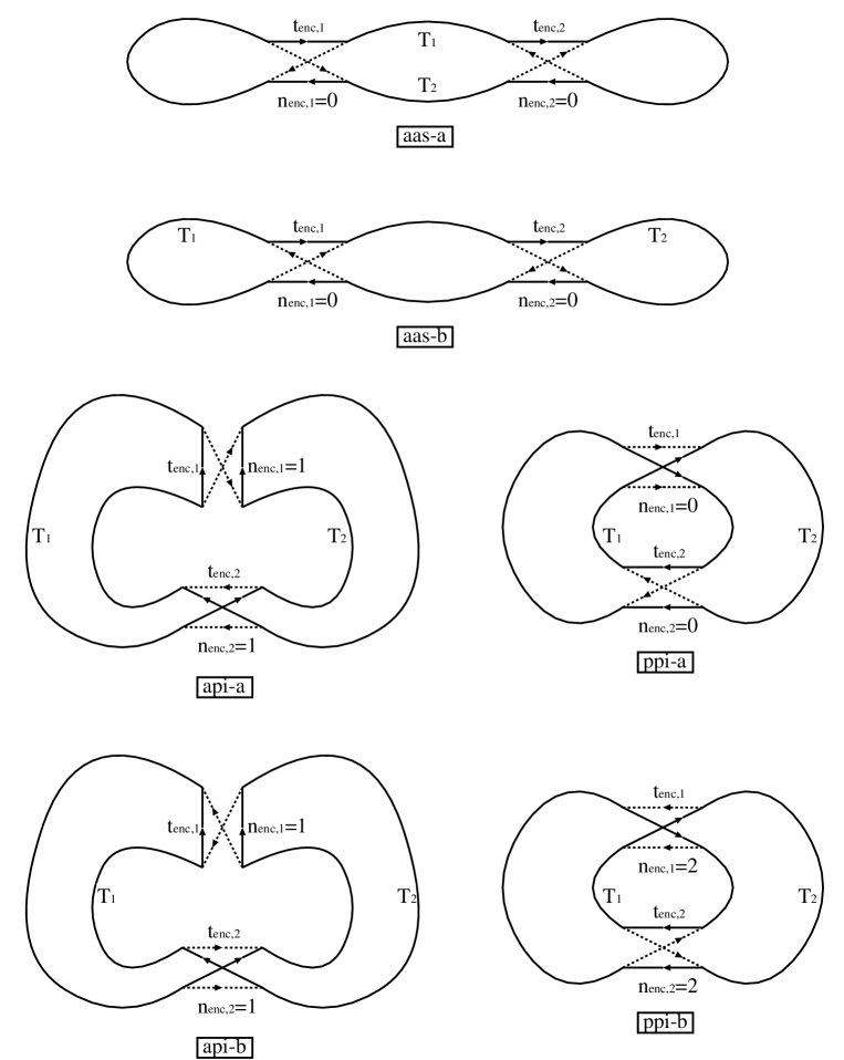
Figure 2: The periodic orbit pairs with two encounters.

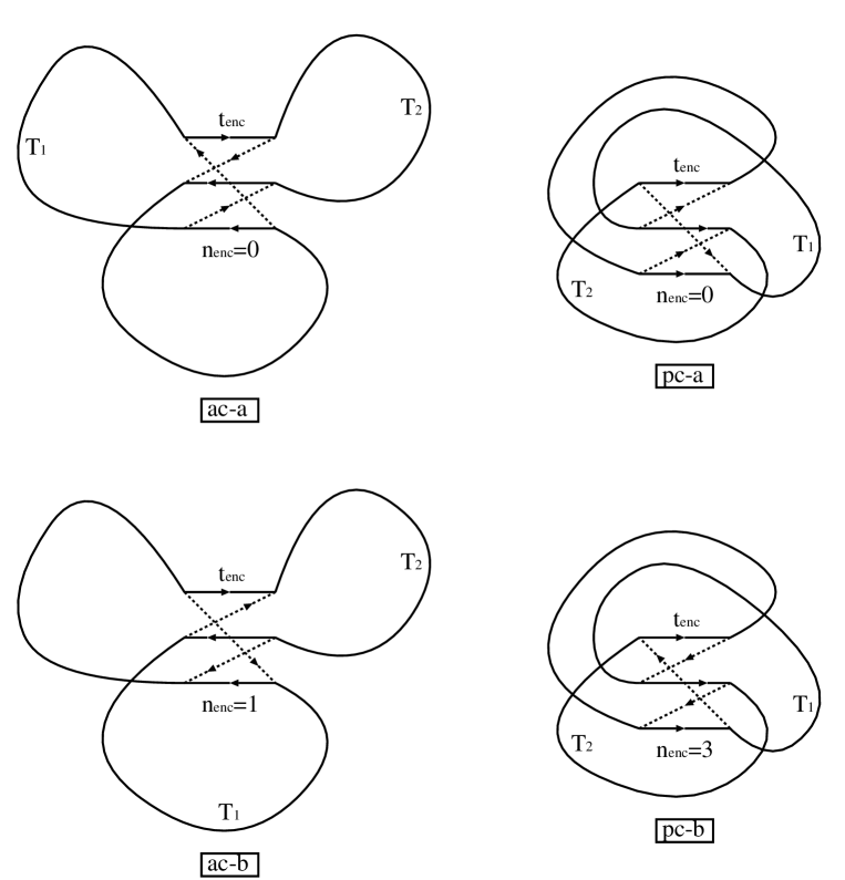
Figure 3: The periodic orbit pairs with one encounter.

References

• [1] O. Bohigas, M.J. Giannoni and C. Schmit, Phys. Rev. Lett. 52 (1984) 1.
• [2] M.V. Berry, Proc. R. Soc. London A400 (1985) 229.
• [3] M. Gutzwiller, Chaos in Classical and Quantum Mechanics (Springer, 1990).
• [4] M. Sieber and K. Richter, Physica Scripta T90 (2001) 128.
• [5] S. Heusler, S. Müller, P. Braun and F. Haake, J. Phys. A37 (2004) L31.
• [6] S. Müller, S. Heusler, P. Braun, F. Haake and A. Altland, Phys. Rev. Lett. 93 (2004) 014103-1.
• [7] S. Müller, S. Heusler, P. Braun, F. Haake and A. Altland, nlin.CD/0503052.
• [8] A. Pandey and M.L. Mehta, Commun. Math. Phys. 87 (1983) 449.
• [9] T. Nagao and K. Saito, Phys. Lett. A311 (2003) 353.
• [10] M. Turek and K. Richter, J. Phys. A36 (2003) L455.
• [11] K. Richter, Semiclassical Theory of Mesoscopic Quantum Systems (Springer, 2000).
• [12] J.H. Hannay and A.M. Ozorio de Almeida, J. Phys. A17 (1984) 3429.
• [13] O. Bohigas, M.-J. Giannoni, A.M. Ozorio de Almeida and C. Schmit, Nonlinearity 8 (1995) 203.
• [14] G. Berkolaiko, H. Schanz and R.S. Whitney, J. Phys. A36 (2003) 8373.
Refer to caption