Generalized BBV Models for Weighted Complex Networks

Abstract

We will introduce two evolving models that characterize weighted complex networks. Though the microscopic dynamics are different, these models are found to bear a similar mathematical framework, and hence exhibit some common behaviors, for example, the power-law distributions and evolution of degree, weight and strength. We also study the nontrivial clustering coefficient $C$ and tunable degree assortativity coefficient $r$, depending on specific parameters. Most results are supported by present empirical evidences, and may provide us with a better description of the hierarchies and organizational architecture of weighted networks. Our models have been inspired by the weighted network model proposed by Alain Barrat et al. (BBV for short), and can be considered as a meaningful development of their original work.

I Introduction

The recent few years have witnessed a great development in physics community to explore and characterize the underlying laws of complex networks, including as diverse as the Internet Internet , the World-Wide Web WWW , the scientific collaboration networks (SCN) CN1 ; CN2 , and world-wide airport networks (WAN)air1 ; air2 . Many empirical measurements have uncovered some general scale-free properties of those real systems, which motivated a wealth of theoretical efforts devoted to the characterization and modelling of them. Since Barabási and Albert introduced their seminal BA model, most efforts have been contributed to study the network topological properties BA . However, networks as well known are far from boolean structures, and the purely topological representation of them will miss important attributes often encountered in real world. For instance, the amount of traffic characterizing the connections of communication systems or large transport infrastructure is fundamental for a full description of them top10 . More recent years, the availability of more complete empirical data and higher computation ability permit scientists to consider the variation of the connection strengths that indeed contain the physical features of many real graphs. Weighted networks can be described by a weighted adjacency $N\times N$ matrix, with element $w_{ij}$ denoting the weight on the edge connecting vertices $i$ and $j$. As a note, this paper will only consider undirected graphs where weights are symmetric. As confirmed by measurements, complex networks often exhibit a scale-free degree distribution $P(k)\thicksim k^{-\gamma}$ with 2$\leq\gamma\leq$3 air1 ; air2 . Interestingly, the weight distribution $P(w)$ is also found to be heavy tailed in some real systems ref1 . As a generalization of connectivity $k_{i}$, the vertex strength is defined as $s_{i}=\sum_{j\in\Gamma(i)}w_{ij}$, where $\Gamma(i)$ denotes the set of $i$’s neighbors. This quantity is a natural measure of the importance or centrality of a vertex in the network. For instance, the strength in WAN provides the actual traffic going through a vertex and is obvious measure of the size and importance of each airport. For the SCN, the strength is a measure of scientific productivity since it is equal to the total number of publications of any given scientist. Empirical evidence indicates that in most cases the strength distribution has a fat tail air2 , similar to that of degree distribution. Highly correlated with the degree, the strength usually displays scale-free property $s\thicksim k^{\beta}$ with $\beta\geq 1$ traffic-driven ; empirical . Driven by new empirical findings, Alain Barrat et al. have presented a simple model (BBV for short) that integrates the topology and weight dynamical evolution to study the dynamical evolution of weighted networks BBV . An obvious virtue of their model is its general simplicity in both mechanisms and mathematics. Thus it can be used as a starting point for further generalizations. It successfully yields scale-free properties of the degree, weight and strength, just depending on one parameter $\delta_{BBV}$ that controls the local dynamics between topology and weights. Inspired by BBV’s work, a class of evolving models will be presented in this paper to describe and study specific weighted networks. This paper is organized as follows: In Section II, we will introduce a traffic-driven model to mimic the weighted technological networks. Analytical calculations are in consistent with numerical results. In Section III, a neighbor-connected model is proposed to study social networks of collaboration, with the comparison of simulations and theoretical prediction as well. At the end of each section, we discuss the differences between the BBV model and ours, from the microscopic mechanisms to observed macroscopic properties. We conclude our paper by a brief review and outlook in Section IV.

II Model A

II.1 The Traffic-Driven Model for Technological Networks

The network provides the substrate on which numerous dynamical processes occur. Technology networks provide large empirical database that simultaneously captures the topology and the traffic dynamics taking place on it. We argue that traffic and its dynamics is a key role for the understanding of technological networks. For Internet, the information flow between routers (nodes) can be represented by the corresponding edge weight. The total (incoming and outgoing) information that each router deals with can be denoted by the node strength, which also represents the importance or load of given router. Our traffic-driven model starts from an initial configuration of $N_{0}$ vertices fully connected by links with assigned weight $w_{0}=1$. The model is defined on two coupled mechanisms: the topological growth and the increasing traffic dynamics:

(i) Topological Growth. At each time step, a new vertex is added with $m$ edges connected to $m$ previously existing vertices (we hence require $N_{0}>m$), choosing preferentially nodes with large strength; i.e. a node $i$ is chosen by the new according to the strength preferential probability:

$$\Pi_{new\rightarrow i}=\frac{s_{i}}{\sum_{k}s_{k}}.$$ (1)

The weight of each new edge is also fixed to $w_{0}=1$. This strength preferential mechanism have simple physical and realistic interpretations in Ref. BBV ; WWX .

(ii) Traffic Dynamics. From the start of the network growing, traffic in all the sites are supposed to constantly increase, with probability proportional to the node strength $s_{i}/\sum_{k}s_{k}$ per step. We assume the growing speed of the network’s total traffic as a discrete constant $W$ (each unit can be considered as an information packet in the case of Internet). Then in statistic sense the newly created traffic in site $i$ per step is

$$\Delta W_{i}=W\frac{s_{i}}{\sum_{k}s_{k}}.$$ (2)

These newly-added packets will be sent out from $i$ to their separate destinations. Our model does not care their specific destinations or delivering paths, but simply suppose that each new packet preferentially takes the route-way with larger edge weight (data bandwidth of links), i.e. with the probability $w_{ij}/s_{i}$, and it hence will increase the traffic (strength) in the corresponding neighbor $j$ of node $i$. It is a plausible mechanism in many real-world webs. For instance, in the case of the airport networks, the potential passenger traffic in larger airports (with larger strength, often located in important cities) will be usually greater than that in smaller airports, and busy airlines often get busier in development. For Internet, routers that have larger traffic handling capabilities are responsible to deal with more information packets. Also, the route-ways with broader data bandwidth will get busier. Admittedly, this “busy get busier” scenario is intuitive in physics, though perhaps not strict in mathematics.

II.2 Analytical Results vs. Numerical Simulations

The model time is measured with respect to the number of nodes added to the graph, i.e. $t=N-N_{0}$, and the natural time scale of the model dynamics is the network size $N$. In response to the demand of increasing traffic, the systems must expand in topology. With a given size, one technological network assumably has a certain ability to handle certain traffic load. Therefore, it could be reasonable to suppose for simplicity that the total weight on the networks increases synchronously by the natural time scale. That is why we assume $W$ as a constant. This assumption also bring us the convenience of analytical discussion WWX . By using the continuous approximation, we can treat $k,w,s$ and the time $t$ as continuous variables. The time evolution of the weights $w_{ij}$ can be computed analytically as follows:

$$\frac{dw_{ij}}{dt} = \Delta W_{i}\frac{w_{ij}}{s_{i}}+\Delta W_{j}\frac{w_{ij}}{s_{j}}$$ (3)

$$= W\frac{s_{i}}{\sum_{k}s_{k}}\frac{w_{ij}}{s_{i}}+W\frac{s_{j}}{\sum_{k}s_{k}}\frac{w_{ij}}{s_{j}}$$

$$= 2W\frac{w_{ij}}{\sum_{k}s_{k}}.$$

The term $\Delta W_{i}w_{ij}/s_{i}$ represents the contribution to weight $w_{ij}$ from site $i$. Considering

$$\sum_{k}s_{k}\approx(2W+2m)t,$$ (4)

one can rewrite the above evolution equation as:

$$\frac{dw_{ij}}{dt}=\frac{W}{W+m}\frac{w_{ij}}{t}.$$ (5)

The link (i,j) is created at $t_{ij}=max(i,j)$ with initial condition $w_{ij}(t_{ij})=1$, so that

$$w_{ij}(t)=\left(\frac{t}{t_{ij}}\right)^{W/(W+m)}.$$ (6)

Further, we can obtain the evolution equations for $s_{i}(t)$ and $k_{i}(t)$:

$$\frac{ds_{i}}{dt} = \sum_{j\in\Gamma(i)}\frac{dw_{ij}}{dt}+m\frac{s_{i}}{\sum_{k}s_{k}}$$ (7)

$$= 2W\frac{\sum_{j}w_{ij}}{\sum_{k}s_{k}}+\frac{ms_{i}}{\sum_{k}s_{k}}$$

$$= (2W+m)\frac{s_{i}}{\sum_{k}s_{k}}$$

$$= \frac{2W+m}{2W+2m}\frac{s_{i}}{t},$$

and

$$\frac{dk_{i}}{dt}=m\frac{s_{i}}{\sum_{k}s_{k}}=\frac{ms_{i}}{2(W+m)t}.$$ (8)

These equations can be readily integrated with initial conditions $k_{i}(t_{i})=s_{i}(t_{i})=m$, yielding

$$s_{i}(t) = m\left(\frac{\;t\;}{\;i\;}\right)^{\frac{2W+m}{2W+2m}},$$ (9)

$$k_{i}(t) = m\frac{2W+s_{i}}{2W+m}.$$ (10)

The strength and degree of vertices are thus related by the following expression

$$s_{i}=\frac{2W+m}{m}k_{i}-2W.$$ (11)

In order to check the analytical predictions, we performed numerical simulations of networks created by the present model with various values of $W$ and minimum degree $m$. In Fig. 1, we report the average strength $s_{i}$ of vertices with connectivity $k_{i}$ and confirm the validity of Eq. (11).

The time $t_{i}=i$ when the node $i$ enters the system is uniformly distributed in $[0,t]$ and the strength probability distribution can be written as

$$P(s,t)=\frac{1}{t+N_{0}}\int_{0}^{t}\delta(s-s_{i}(t))dt_{i},$$ (12)

where $\delta(x)$ is the Dirac delta function. Using equation $s_{i}(t)\sim(t/i)^{a}$ obtained from Eq. (9), one obtains in the infinite size limit $t\rightarrow\infty$ the power-law distribution $P(s)\sim s^{-\gamma_{{}_{A}}}$ (as shown in Fig. 2) with

$$\gamma_{{}_{A}}=1+\frac{1}{a}=2+\frac{m}{2W+m}.$$ (13)

Obviously, when $W=0$ the model is topologically equivalent to the BA network and the value $\gamma_{{}_{A}}=3$ is recovered. For larger values of $W$, the distribution is gradually broader with $\gamma_{{}_{A}}\rightarrow 2$ when $W\rightarrow\infty$. Since $s$ and $k$ are proportional, one can expect the same behavior of degree distribution $P(k)\sim k^{-\gamma_{{}_{A}}}$. Analogously, the weight distribution can be calculated yielding the scale-free property $P(w)\sim w^{-\alpha_{{}_{A}}}$, with the exponent $\alpha_{{}_{A}}=2+m/W$ (See Fig. 3).

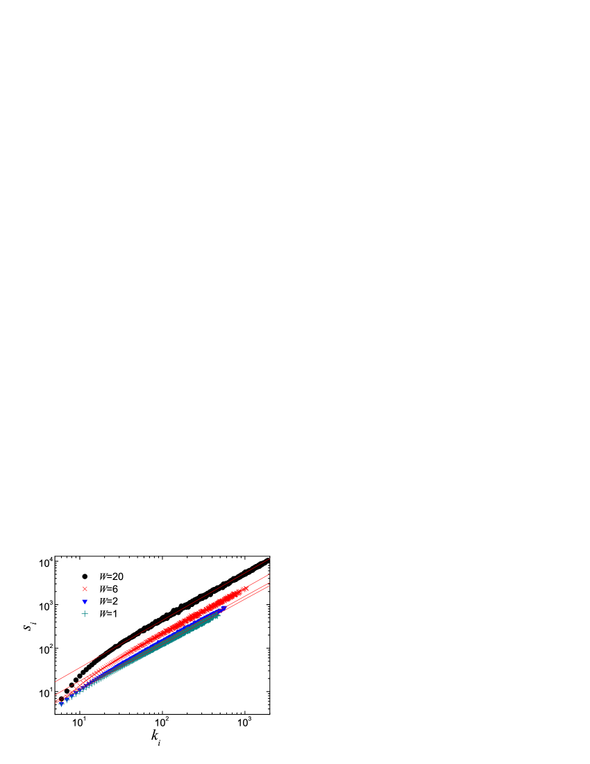
Figure 1: The average strength $s_{i}$ of the nodes with connectivity $k_{i}$ for different $W$ (log-log scale). Linear data fittings all give slope $1.00\pm 0.02$, demonstrating the predicted linear correlation between strength and degree.

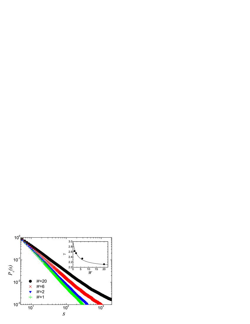
Figure 2: Cumulative strength probability distribution $P_{c}(s)$ with various $W$. Data agree well with the power-law form $s^{-\gamma_{{}_{A}}}$. The inset reports $\gamma_{{}_{A}}$ from data fitting (filled circles), in comparison with the theoretical prediction $\gamma_{{}_{A}}=2+\frac{m}{2W+m}=2+\frac{5}{2W+5}$(line), averaged over 20 independent networks of size N=7000.

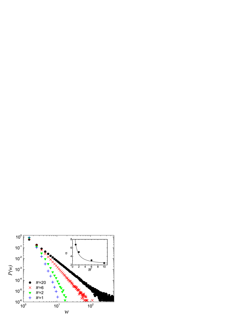
Figure 3: Weight probability distribution $P(w)$ with various values of $W$. Data are consistent with a power-law behavior $w^{-\alpha_{{}_{A}}}$. In the inset we give the value of $\alpha_{{}_{A}}$ obtained by data fitting (filled circles), together with the analytical expression $\alpha_{{}_{A}}=2+m/W=2+5/W$(line). The data are averaged over 20 independent realizations of network size N=7000.

II.3 Clustering and Correlations

A complete characterization of the network structure must take into account the level of clustering and degree correlations present in the network. Information on the local connectedness is provided by the clustering coefficient $c_{i}$ defined for any vertex $i$ as the fraction of connected neighbors of $i$. The average clustering coefficient $C=N^{-1}\sum_{i}c_{i}$ thus expresses the statistical level of cohesiveness measuring the global density of interconnected vertices’ triples in the network. Further information can be gathered by inspecting the average clustering coefficient $C(j)$ restricted to classes of vertices with degree $k$:

$$C(k)=\frac{1}{NP(k)}\sum_{i/k_{i}=k}c_{i}.$$ (14)

In many networks, $C(k)$ exhibits a power-law decay as a function of $k$, indicating that low-degree nodes generally belong to well interconnected communities (high clustering coefficient) while high-degree sites are linked to many nodes that may belong to different groups which are not directly connected (small clustering coefficient). This is generally the signature of a nontrivial architecture in which hubs (high degree vertices) play a distinct role in the network. Correlations can be probed by inspecting the average degree of the nearest neighbors of a vertex $i$, that is, $k_{nn,i}=k_{i}^{-1}\sum_{j}k_{j}$. Averaging this quantity over nodes with the same degree $k$ leads to a convenient measure to investigate the behavior of the degree correlation function

$$k_{nn}(k)=\frac{1}{NP(k)}\sum_{i/k_{i}=k}k_{nn,i}=\sum_{k^{\prime}}k^{\prime}P(k^{\prime}|k),$$ (15)

If degrees of neighboring vertices are uncorrelated, $P(k^{\prime}|k)$ is only a function of $k^{\prime}$ and thus $k_{nn}(k)$ is a constant. When correlations are present, two main classes of possible correlations have been identified: assortative behavior if $k_{nn}(k)$ increases with $k$, which indicates that large degree vertices are preferentially connected with other large degree vertices, and disassortative if $k_{nn}(k)$ decreases with $k$. The above quantities provide clear signals of a structural organization of networks in which different degree classes show different properties in the local connectivity structure. Almost all the social networks empirically studied show assortative mixing pattern, while all others including technological and biological networks are disassortative. The origin of this difference is not understood yet. To describe these types of mixing, Newman further proposed some simpler measures, which is called assortativity coefficients mixing . In this paper, we will also use the formula proposed by Newman mixing ,

$$r=\frac{M^{-1}\sum_{i}j_{i}k_{i}-[M^{-1}\sum_{i}\frac{1}{2}(j_{i}+k_{i})]^{2}}{M^{-1}\sum_{i}\frac{1}{2}(j_{i}^{2}+k_{i}^{2})-[M^{-1}\sum_{i}\frac{1}{2}(j_{i}+k_{i})]^{2}},$$ (16)

where $j_{i}$, $k_{i}$ are the degrees of vertices at the ends of the $i$th edges, with $i=1,...,M$ ($M$ is the total number of edges in the observed graph). Simply, $r>0$ means assortative mixing, while $r<0$ implies disassortative pattern.

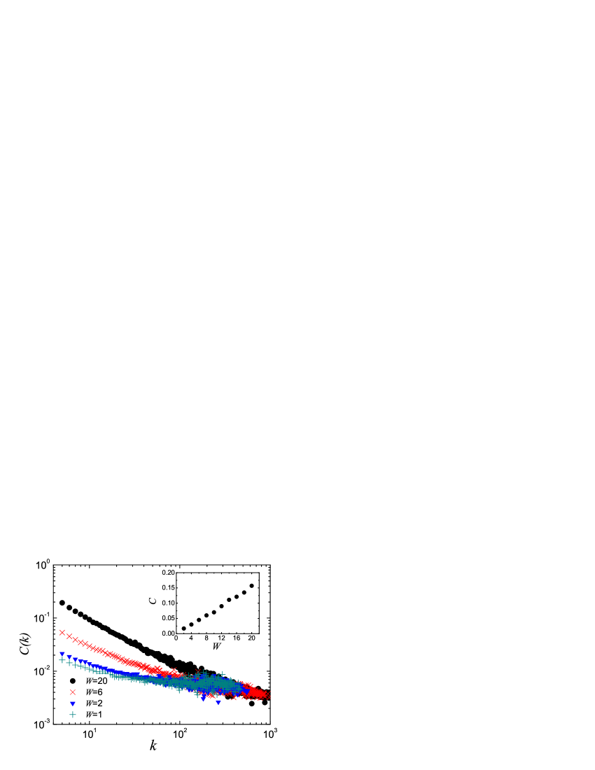
Figure 4: The scaling of $C(k)$ with $k$ for various $W$. The data are averaged over 20 independent runs of network size N=7000. The inset shows the average clustering coefficient $C$, depending on increasing $W$.

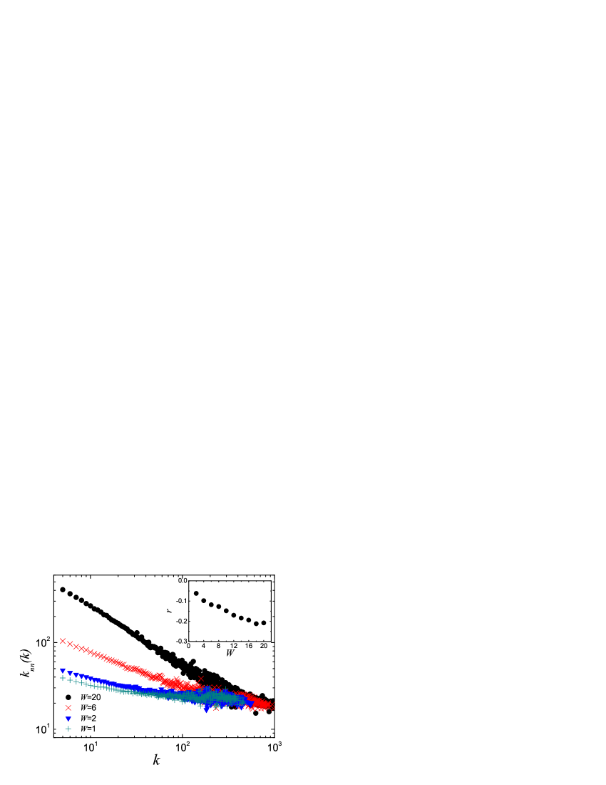
Figure 5: Average connectivity $k_{nn}(k)$ of the nearest neighbors of a node depending on its connectivity $k$ for different $W$. The data are averaged over 20 network realizations of N=7000. The assortativity coefficient $r$ depending on $W$ is shown in the inset.

In order to inspect the above properties we perform simulations of graphs generated by the model for different values of $W$, fixing $N=7000$ and $m=5$. In the case of clustering, the model also exhibits properties which are depending on the basic parameter $W$. More precisely, for small $W$, the clustering coefficient of the network is small and $C(k)$ is flat. As $W$ increases however, the global clustering coefficient increases and $C(k)$ becomes a power-law decay similar to real network data hierarchy . Fig. 4 shows that the increase in clustering is determined by low-degree vertices. The average clustering coefficient $C$ is found to be a function of $W$, as shown in its inset. This numerical result obviously demonstrates the important effect of traffic on the hierarchical structure of technological networks. Analogous properties are obtained for the degree correlation spectrum. For small $W$, the average nearest neighbor degree $k_{nn}(k)$ is quite flat as in the BA model. The disassortative character emerges as $W$ increases and gives rise to a power law behavior of $k_{nn}(k)\sim k^{-\eta}$ (Fig. 5). The assortativity coefficient $r$ versus $W$, as reported in the inset of Fig. 5, demonstrates the tunable disassortative property of this model, which is supported by measurements in real technological networks Internet . The qualitative explanations of the correlations and clustering spectrum can be found in BBV2 , and their theoretical analysis appears in BP . In sum, all the simulation results for clustering and degree correlation, as empirically observed, imply us that the increasing traffic may be the driven force to shape the hierarchical and organizational structure of real technological networks.

II.4 Comparison with the BBV model

One may notice that if the parameter $W$ is replaced by $W=m\delta_{{}_{A}}$, then the mathematical framework of our traffic-driven model is equivalent to that of BBV’s BBV2 , though the specific weights’ dynamics are quite different between the two. By comparison with $\delta_{{}_{BBV}}$ (that is, the fraction of weight which is locally “induced” by the new edge onto the neighboring others), the parameter $\delta_{{}_{A}}$ in our model, with macroscopic perspectives, is the ratio of the total weight increment on the expanding structure (W) to the number of newly-established links (m) at each time step. It is an important measure for the relative growing speed of traffic vs. topology, and controls a series of the network scale-free properties. Thus, there is an obvious difference between BBV model and ours: the former is based on the local rearrangement of weights induced by newly added links, while the latter is built upon the global traffic growth and the redistribution of weights according to the local nature of network. Noticeably, the weight dynamical evolution of the BBV model is triggered only by newly added vertices, hardly resulting in satisfying interpretations to collaboration networks or the airport systems. For these two cases, even if the size of networks keeps invariant, co-authored papers will still come out and airports can become more crowded as well. In contrast, this difficulty for practical explanations naturally disappear in our model, due to its global weight dynamics. Above all, the traffic-driven model here, without loss of simplicity and practical senses, has generalized BBV’s work and narrowed its applicable scope to technological networks. Based on it, more complicated variations of the microscopic rules may be implemented to better mimic technological networks. Especially worth remarking is that the present empirical studies on airport networks and Internet indicate the nonlinear degree-strength correlation $s\sim k^{\beta}$ with $\beta>1$. In Ref. BBV2 , Barrat et al. proposed the heterogeneous coupling mechanism to obtain this property. This is not difficult to introduce into the present traffic-driven version. Moreover, we find that the nontrivial weight-topology correlation can also emerge from the accelerating growth of traffic weight BH or from the accelerating creation and reinforcement of internal edges WWX ; BH .

III Model B

III.1 The Neighbor-Connected Model for Social Networks

Social networks are a paradigm of the complexity of human interactions, which have also attracted a great deal of attention within the statistical physics community. The study of social networks has been traditionally hindered by the small size of the networks considered and the difficulties in the process of data collection (usually from questionnaires or interviews). More recently, however, the increasing availability of large databases has allowed scientists to study a particular class of social networks, the so-called collaboration networks. The co-authorship network of scientists represents a prototype of complex evolving networks, which can be defined in a clear way. Their large size has allowed researchers to get a reliable statistical description of their topological and weight properties, and hence reach reliable conclusions of the network structure and dynamics. In weighted social networks, the edge weight between a pair of nodes can represent the tightness of their connection. The larger weight indicates the more frequency of interaction; e.g. the number of co-authored papers between two scientists, the frequency of telephone or email contacts between two acquaintances, etc. In addition, it is more probable that two vertices with a common neighbor get connected than two vertices chosen at random. Clearly, this property leads to a large average clustering coefficient since it increases the number of connections between the neighbors of a vertex. This is already observed in a model proposed by Davidsen, Ebel and Bornhodt DEB .

Our neighbor-connected model starts from an initial graph of $N_{0}$ vertices, fully connected by links with assigned weight $w_{0}=1$. Its evolution then is simply based on the dynamics of connecting nearest-neighbors: At each time step, a new vertex $n$ is added with one primary link and $m$ secondary links, which connect with $m+1$ existing vertices (the initial network configuration hence requires $N_{0}>m+1$). Actually, the newly-built connections are not independent, but related with each other. The primary link ($w_{0}=1$) first preferentially attaches to an old node with large strength; i.e. a node $i$ is connected by the primary link with probability

$$\Pi_{n\rightarrow i}=\frac{s_{i}}{\sum_{k}s_{k}}.$$ (17)

Then, the $m$ secondary connections (assigned $w_{0}=1$ each) are preferentially built between the new vertex and $m$ neighbors of node $i$, with the weight preferential probability

$$\Pi_{n\rightarrow j}=\frac{w_{ij}}{s_{i}},$$ (18)

where $j\in\Gamma(i)$. After building the primary link $(n,i)$, the creation of every secondary link $(n,j)$ is assumed to introduce variations of network weights. For the sake of simplicity, we limit ourselves to the case where the introduction of a primary link on node $i$ will trigger only local rearrangement of weights on the existing neighbors $j\in\Gamma(i)$, according to the rule

$$w_{ij}\rightarrow w_{ij}+\delta.$$ (19)

In general, $\delta$ depends on the local dynamics and can be a function of different parameters such as the weight $w_{ij}$, the degree or the strength of $i$, etc. In the following, we will simply focus on the case that $\delta=const$. After the weights have been updated, the evolving process is iterated by introducing a new vertex until the desired size of the network is reached.

The above mechanisms have simple physical and realistic interpretations. Once a fresh member joins a social community, he will be introduced to his neighbors or take initiatives to interact with them. Then, his social connections will soon be built within his neighborhood. It is reasonable that the entering of this new member can trigger the local variation of connections. Take the SCN for example, a scientist joining a research group will often collaborate with both the group director (primary link) and the other group members (secondary links). The scientist’s affiliation can naturally boost the research productivity of the group and also, enhance the collaborations of other members. The above scenario may be a best interpretation of the origin of our model parameter $\delta$. We use $\delta$ to control the effect of the newly-introduced member on the weights of connections among the local neighbors. In the proceeding section, we will see the model also gives a wealth of scale-free behaviors depending on this basic parameter.

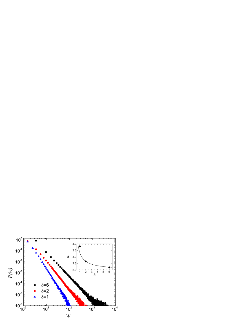
Figure 6: Weight probability distribution with m=3. Data are consistent with a power-law behavior $P(w)\sim w^{-\alpha_{{}_{B}}}$. In the inset we give the value of $\alpha_{{}_{B}}$ obtained by data fitting (filled circles), together with the analytical form Eq. (22) (line). The data are averaged over 100 independent realizations of network size N=7000.

III.2 Analytical and Numerical Results

Along the analytical lines used in Section II, one can also calculate the time evolution of the strength, weight and degree, and hence calculated their scale-free distributions as follows:

$$\frac{dw_{ij}}{dt}=\frac{ms_{i}}{\sum_{k}s_{k}}\frac{w_{ij}}{s_{i}}\delta+\frac{ms_{j}}{\sum_{k}s_{k}}\frac{w_{ij}}{s_{j}}\delta=2m\delta\frac{w_{ij}}{\sum_{k}s_{k}}.$$ (20)

By noticing $\sum_{k}s_{k}\approx 2(m+1)t+2m\delta t=2(1+m+m\delta)t$, we have

$$\frac{dw_{ij}}{dt}=\frac{m\delta}{1+m+m\delta}\frac{w_{ij}}{t}=\theta\frac{w_{ij}}{t},$$ (21)

and so that $w_{ij}(t)=(t/t_{ij})^{\theta}$, which indicates the power-law distribution of weight $P(w)\sim w^{-\alpha_{{}_{B}}}$ with exponent

$$\alpha_{{}_{B}}=1+\frac{1}{\theta}=2+\frac{1+m}{m\delta}.$$ (22)

Further, the evolution equations for $s_{i}$ and $k_{i}$ are obtained

$$\frac{ds_{i}}{dt} = \sum_{j}\frac{dw_{ij}}{dt}+\frac{s_{i}}{\sum_{k}s_{k}}+\sum_{j\in\Gamma(i)}\frac{s_{j}}{\sum_{k}s_{k}}m\frac{w_{ij}}{s_{j}}$$ (23)

$$= 2m\delta\frac{\sum_{j}w_{ij}}{\sum_{k}s_{k}}+(m+1)\frac{s_{i}}{\sum_{k}s_{k}}$$

$$= \frac{1+m+2m\delta}{2+2m+2m\delta}\frac{s_{i}}{t}=\lambda\frac{s_{i}}{t},$$

$$\frac{dk_{i}}{dt} = \frac{s_{i}}{\sum_{k}s_{k}}+\sum_{j\in\Gamma(i)}\frac{s_{j}}{\sum_{k}s_{k}}m\frac{w_{ij}}{s_{j}}$$ (24)

$$= \frac{m+1}{2+2m+2m\delta}\frac{s_{i}}{t}.$$

Integrating with the initial conditions $k_{i}(t=i)=s_{i}(t=i)=m+1$, we have

$$s_{i}(t) = (m+1)\left(\frac{\;t\;}{\;i\;}\right)^{\lambda}$$

$$k_{i}(t) = (m+1)\frac{s_{i}(t)+2m\delta}{1+m+2m\delta},$$ (25)

which determine the scale-free distributions of both strength and degree, with the same power-law exponent

$$\gamma_{{}_{B}}=1+\frac{1}{\lambda}=2+\frac{1+m}{1+m+2m\delta}.$$ (26)

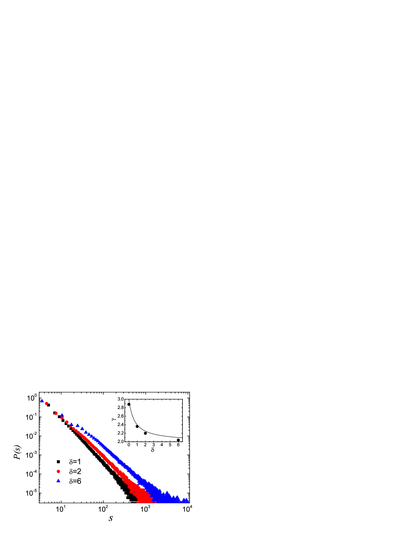
Figure 7: Strength probability distribution with m=3. Data agree well with the power-law form $P(s)\sim s^{-\gamma_{{}_{B}}}$. The inset reports $\gamma_{{}_{B}}$ from data fitting (filled circles) averaged over 100 independent networks of size N=7000, in comparison with the theoretical prediction Eq. (26) (line).

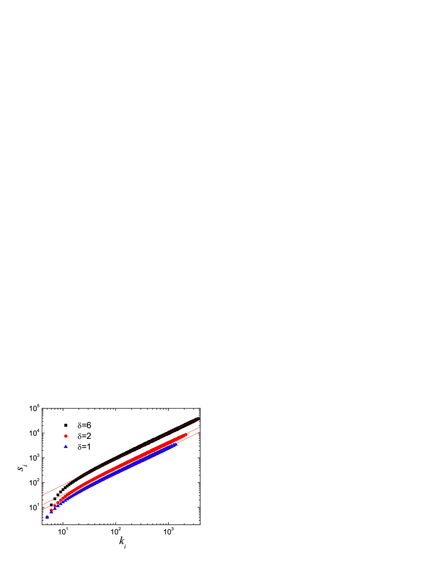
Figure 8: The average strength $s_{i}$ of vertices with connectivity $k_{i}$ for different $\delta$ with m=3 (log-log scale). Linear data fittings all give slope $1.00\pm 0.02$, confirming the prediction $\beta=1$.

We also performed numerical simulations of networks generated by the model with various values of $\delta$ and minimum degree $m$. As one can see, Fig. 6 and 7 recover the theoretical predictions for scale-free distributions of weight and strength, and Fig. 8 validates the linear strength-degree correlation. It is worth stressing that the empirical evidence in co-authorship networks just indicates the linear correlation $s\sim k$ air2 .

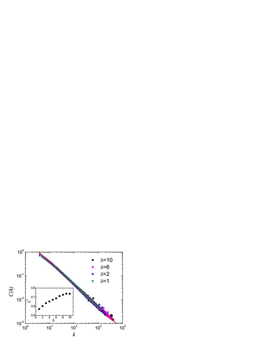
Figure 9: The scaling of $C(k)$ with $k$ for various $\delta$ with m=3. Their fitted power-law exponents all give 0.94 (dashed line). The data are averaged over 100 independent runs of network size N=7000. The inset shows the average clustering coefficient $C$ depending on increasing $\delta$.

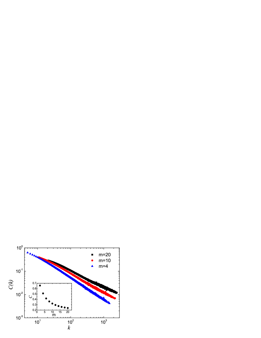
Figure 10: The scaling of $C(k)$ with $k$ for various $m$ with $\delta=1$. The data are averaged over 100 independent runs of network size N=7000. The inset shows the average clustering coefficient $C$ depending on increasing $m$.

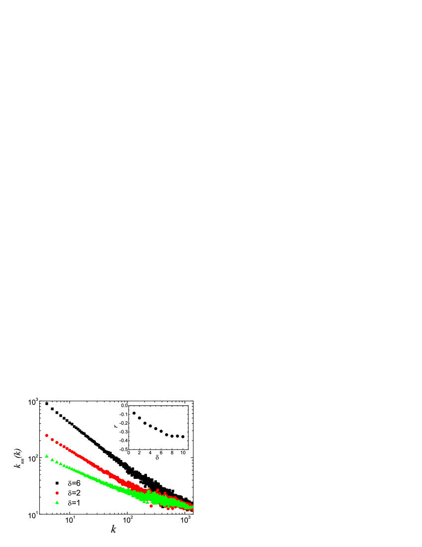
Figure 11: Average connectivity $k_{nn}(k)$ of the nearest neighbors of a node depending on its connectivity $k$ for different $\delta$ with m=3. The data are averaged over 100 network realizations of N=7000. The assortativity coefficient $r$ versus $\delta$ is also reported in the inset.

III.3 Discussions

There are two important differences between the BBV model and our neighbor-connected one, though the latter can be regarded as an interesting variation of the former. First, in the BBV model the evolution and distributions of such quantities as strength, weight and degree are simply depending on the parameter $\delta_{{}_{BBV}}$ which controls the coupling between local topology and weights. In our model, however, the evolution and distributions of those quantities are controlled by two parameters ($\delta$ and $m$, as reflected in theoretical part), which together determine the effect of the new node on the local weights and topology. Though we have fixed $m$ in most simulations, the role of parameter $m$ should not be ignored. As Fig. 9 reports, the curvature of $C(k)$ is not sensitive to the variations of $\delta$, but it nontrivially depends on $m$ as shown in Fig. 10. Second, given the same minimum degree, the average clustering coefficient $C$ of our neighbor-connected model (see the inset of Fig. 9) can be much larger than that of BBV’s model or of our Model A, because the secondary links in Model B considerably increase the density of triangles within the system. Compared with the original model, this larger clustering demonstrate an important advantage of Model B in modelling the small-world property of real complex networks. One question arises from the inset of Fig. 10: at first sight, it may be surprising to see that $C$ greatly decreases when increasing the secondary linking number $m$. Actually, larger $m$ in the model means larger minimum degree. When a new node arrives, the number of triangles in the system will increase by $m$. But for a smallest-degree node $i$, its clustering is $c_{i}(m)=2N_{\vartriangle}(i)/m(m+1)$ where $N_{\vartriangle}(i)$ denotes the number of connected neighbors of node $i$. Therefore, increasing $m$, we will decrease $c_{i}$ more greatly, resulting in the decaying of $C$. Admittedly, there still exists a common point which leads to the restriction of Model B to mimic and interpret social networks. The degree correlations in both models are negative (see the inset of Fig. 11), indicating their disassortative mixing patten that is opposite in social networks. Is it possible to find out a unified minimum model to characterize both the assortative and disassortative networks? This question is very challenging and appears among the leading ones in front of network researchers top10 . Our recent studies may shed some new light on this tackling problem WangHu . Anyway, the present neighbor-connected model (though disassortative) has maintained the simplicity of the BBV model and appears as a more specific version for weighted social networks, considering its larger clustering and clearer hierarchical structure.

IV Review and outlook

In this paper, we have presented and studied two evolving models for weighted complex networks. These two models intend to mimic technological networks and social graphs respectively, and can be regarded as a meaningful development of the original BBV model. Though their specific evolution dynamics are different, all of them are found to bear similar mathematical structures and hence exhibit several common behaviors, e.g. the power-law distributions and evolution of degree, weight and strength. In each case, we also studied the nontrivial clustering coefficient $C$ and tunable degree assortativity $r$ as well as their degree-dependent correlations. In such context, we compared our generalized models with the original one, and got several interesting conclusions, which may provide us with a better understanding of the hierarchical and organizational architecture of weighted networks. For all the above reasons, we would like to classify these models into a class, within which the BBV’s is the first one and may be the simplest one. It must be admitted that this class of models do not take into account the internal connections during the network evolution, which is yet beyond the scope of this paper. Still, we hope that our generalized work can make this model family more diversified and help bring it some new sights.

References

- (1) R. Pastor-Satorras and A. Vespignani, Evolution and Structure of the Internet: A Statistical Physics Approach (Cambridge University Press, Cambridge, England, 2004).
- (2) R. Albert, H. Jeong, and A.-L. Barabási, Nature 401, 130 (1999).
- (3) M.E.J. Newman, Phys. Rev. E 64, 016132 (2001).
- (4) A.-L. Barabási, H. Jeong, Z. Néda. E. Ravasz, A. Schubert, and T. Vicsek, Physica (Amsterdam) 311A, 590 (2002).
- (5) R. Guimera, S. Mossa, A. Turtschi, and L.A.N Amearal, cond-mat/0312535.
- (6) A. Barrat, M. Barthélemy, R. Pastor-Satorras, and A. Vespignani, Proc. Natl. Acad. Sci. U.S.A. 101, 3747 (2004).
- (7) R. Albert and A.-L. Barabási, Rev. Mod. Phys. 74, 47 (2002).
- (8) A virtual round tabel on ten leading questions for network research can be found in the special issue on Applications of Networks, edited by G. Caldarelli, A. Erzan and A. Vespignani [Eur. Phys. J. B 38, 143 (2004)].
- (9) W. Li and X. Cai, Phys. Rev. E 69, 046106 (2004).
- (10) K.-I. Goh, B. Kahng, and D. Kim, cond-mat/0410078 (2004).
- (11) R. Pastor-Satorras, A. Vázquez, and A. Vespignani, Phys. Rev. Lett. 87, 258701 (2001).
- (12) A. Barrat, M. Barthélemy, and A. Vespignani, Phys. Rev. Lett. 92, 228701 (2004).
- (13) W.-X. Wang, B.-H. Wang, B. Hu, G. Yan, and Q. Ou, Phys. Rev. Lett. 94, 188702 (2005).
- (14) M. E. J. Newman, Phys. Rev. E 67, 026126 (2003).
- (15) E. Ravasz and A.-L Barabási, Phys. Rev. E 67, 026112 (2003).
- (16) A. Barrat, M. Barthélemy, and A. Vespignani, Phys. Rev. E 70, 066149 (2004).
- (17) A. Barrat and R. Pastor-Satorras, Phys. Rev. E 71, 036127 (2005).
- (18) B. Hu et al. (unpublished).
- (19) J. Davidsen, H. Ebel, and S. Bornhodt, Phys. Rev. Lett. 88, 128701 (2001).
- (20) W.-X. Wang, B. Hu, B.-H. Wang, and G. Yan (unpublished).