Scarred Resonances and Steady Probability Distribution in a Chaotic Microcavity

Abstract

We investigate scarred resonances of a stadium-shaped chaotic microcavity. It is shown that two components with different chirality of the scarring pattern are slightly rotated in opposite ways from the underlying unstable periodic orbit, when the incident angles of the scarring pattern are close to the critical angle for total internal reflection. In addition, the correspondence of emission pattern with the scarring pattern disappears when the incident angles are much larger than the critical angle. The steady probability distribution gives a consistent explanation about these interesting phenomena and makes it possible to expect the emission pattern in the latter case.

Directional lasing emission from a microcavity has been intensively studied in the last decade due to its direct application to optical communications and optoelectronic circuitsbook1 . The first realization of the directional emission has been achieved in the microcavities which are slightly deformed from circle or sphereno97 . In the slightly deformed microcavities it is known that the light is emitted from a boundary point of the highest curvature and the direction is tangential to the boundary. In ray dynamical viewpoint, this is a result of tunneling of the rays confined in the Kolmogorov-Arnold-Moser tori through the lowest dynamical barrier.

As the microcavity is strongly deformed, the ray dynamics inside becomes chaotic and lasing modes from the chaotic cavity can be expected to have complicated patterns without any directionality due to the complexity of the corresponding ray trajectories. However, the openness of the microcavity enhances the scarring phenomenonHe84 , localization along unstable periodic orbits, and the scarred resonance shows a strong directional emission from the chaotic microcavity. The scarred lasing modes are observed in several experimental studiesscar ; Re02 , and the emission direction from the scarred mode can be nontangential due to the Fresnel filtering effectRe02 .

In a recent studyLee04 , it was reported that in a spiral-shaped chaotic microcavity there are many resonances showing special localized patterns, so-called quasiscarred resonances which have, unlike typical scarred resonances, no underlying unstable periodic orbit. This finding indicates that the openness of the system plays a crucial role in the formation of localized pattern, and implies that the properties of openness should be imprinted in scarred resonances also. It is quite interesting and important to uncover the mechanism of how the openness of the microcavity can change the scarred resonance pattern and can determine the emission direction. This is the motivation of our study.

In this Letter, we illustrate characteristics of the scarred resonances in a chaotic microcavity of stadium shape and show that the scarred resonances can be classified into two categories, i.e., type-I and II for convenience, based on their difference in emission property. The type-I scarred resonances have a clear correspondence of the emission pattern with the scarring pattern, e.g., the bouncing point of the scarring pattern matches well with the emitting point. However, in the type-II scarred resonances there is no correspondence between emission and scarring patterns, and the emission pattern is determined by the structure of steady probability distribution (SPD)Lee04 near the critical line ($p_{c}=\sin\theta_{c}=1/n$, $n$ being the refractive index) for total internal reflection. Moreover, the SPD provides a consistent explanation about a novel feature of the type-I scarred resonances, i.e., the spatial splitting phenomenon of different chiral components of the scarring pattern.

It is known that long time ray dynamical properties of a chaotic microcavity can be described by the SPD, $P_{s}(s,p)$, which is the spatial part of the exponentially decaying survival probability distribution in phase space $(s,p)$, where $s$ is the boundary coordinate and $p=\sin\theta$, $\theta$ being incident angleLee04 . In chaotic microcavities this SPD is a useful tool in identifying both the structure of openness and the escaping mechanism of ray trajectories. In addition, various informations about the long time ray dynamics can be easily calculated from the SPD, e.g., the ray dynamical far field distribution is given by

$$P_{far}(\phi)\propto\int dsdp\,P_{s}(s,p)\,{\cal T}(p)\,\delta(\phi-f(s,p)),$$ (1)

where ${\cal T}(p)$ is the transmission coefficientbook2 and the far field angle $\phi$ is given as $f(s,p)$ determined by the geometry of boundary and Snell’s law. This $P_{far}(\phi)$ would correspond to the averaged far field distribution for the resonances with relatively high quality factor $Q$. Even in the case of individual resonance pattern, the SPD provides a background structure in phase space and is useful to understand the resonance pattern and its emission property.

As a phase space representation of a quantum mechanical eigenfunction, the Husimi function has been widely used in billiard systemsBa04 . For dielectric microcavities, Hentschel et al.He03 have developed the incident and the reflective Husimi functions as

$$H^{inc(refl)}(s,p)=\frac{k}{2\pi}\left|-{\cal F}h(s,p)+(-)\frac{i}{k{\cal F}}h^{\prime}(s,p)\right|^{2},$$ (2)

where the weighting factor is ${\cal F}=\sqrt{n\sqrt{1-p^{2}}}$ and the components of the Husimi function are given as $h(s,p)=\int ds^{\prime}\psi(s^{\prime})\xi(s^{\prime};s,p)$, $h^{\prime}(s,p)=\int ds^{\prime}\partial\psi(s^{\prime})\xi(s^{\prime};s,p)$, respectively. $\psi(s)$ and $\partial\psi(s)$ are the boundary wavefunction and its normal derivative, and $\xi(s^{\prime};s,p)$ is the minimal-uncertainty wave packet of the form

$$\xi(s^{\prime};s,p)=\sum_{l}\frac{1}{\sqrt{\sigma\sqrt{\pi}}}\exp[-\frac{1}{2\sigma^{2}}(s^{\prime}-s)^{2}-ikp(s^{\prime}+Ll)]$$ (3)

where $k$ and $L$ are the wavenumber inside the cavity and the total length of boundary, respectively. This corresponds to a Gaussian wavefunction centered at $(s,p)$, and we set the aspect ratio factor as $\sigma=(\sqrt{2}/k)^{-1/2}$ throughout this Letter. This formalism for Husimi functions is exact in the high $k$ limit,and it still gives good approximates around $kR\simeq 90$ where our calculation is performed.

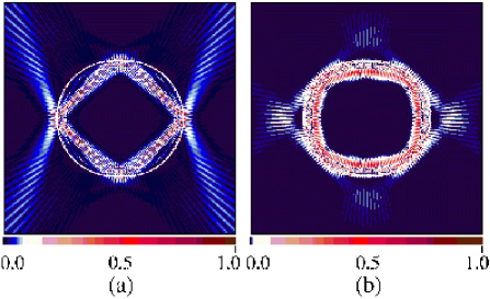
Figure 1: (color online) The type-I scarred resonances showing a diamond (a) and a rectangle (b) scarring patterns in a stadium-shaped microcavity with $n=\sqrt{2}$. Note that the refractive emissions come out from the bouncing points of the scarring patterns. The resonance positions are (a) $kR=(91.68,-0.17)$ and (b) $kR=(92.48,-0.035)$.

As shown in Fig. 1, by using the boundary element method (BEM)Wie03 we obtain two examples of type-I scarred resonances, where scarring patterns are diamond (a) and rectangle (b), for a stadium-shaped microcavity with 0.2$R$ length of linear segment, $R$ being the radius of two semicircles. It is clear that the emitted light is refracted out from the bouncing points of the scarring patterns inside the microcavity. We also obtain the Husimi functions $H^{inc(refl)}(s,p)$(Eq.(2)), where the origin of $s$ is the right end of the stadium. Figure 2 shows the incident Husimi functions $H^{inc}(s,p)$ from which we can realize two characteristics of the type-I scarred resonances. First, the critical lines, $p=\pm p_{c}$, cross the localized spots, which explains why the emission pattern matches with the scarring pattern inside. This also implies that the type-I scarred resonances are somewhat leaky, i.e., relatively low $Q$ resonances. The second is that peak positions $(s^{in\pm}_{i},p^{in\pm}_{i})$ ($i=1,2,3,4$) of the localized spots in $H^{inc}(s,p)$ are not located on the expected positions $(s^{*}_{i},\pm p^{*}_{i})$ (black dots in Fig.2) from the corresponding periodic ray orbits. They are slightly shifted in opposite ways depending on the chirality of propagating component. Moreover, the direction of the shift appears to be opposite in both scarred resonances, e.g., for positive chiral component ($p>0$) the shift, $\delta s^{+}_{i}=s^{in+}_{i}-s^{*}_{i}$, is negative for the diamond case and positive for the rectangle case.

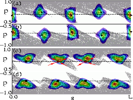
Figure 2: (color online) The $H^{inc}(s,p)$ of the type-I scarred resonances in Fig.1. (a) and (b) diamond scarring case. (c) and (d) rectangle scarring case. The SPD is shown by the gray dots and the critical line $p_{c}$ is denoted by the dashed line. The bouncing positions $(s^{*}_{i},\pm p^{*}_{i})$ expected from the diamond and rectangle ray periodic orbits are pointed as black dots.

In the case of a chaotic billiard, the Husimi function of a scarred eigenfunction shows localization on an unstable periodic orbit and along nearby stable and unstable manifolds, and the resulting hyperbolic localization reflects that the system has the time-reversal symmetryLee03 . However, in the chaotic microcavity case the openness breaks the time-reversal symmetry and makes some structure in the phase space, i.e., the structure of the SPD. The SPD structure of the present system is shown in the background in Fig. 2. We note that the expected ray positions $(s^{*}_{i},\pm p^{*}_{i})$ are on the edge of the structure near the critical line, and the localized spots of $H^{inc}(s,p)$ are shifted toward the denser part of the SPD structure. This shift can be understood from the fact that the rays in the denser part contribute strongly to the interference process for formation of a resonance since the denser part of the SPD corresponds to the rays surviving longer time.

A more direct explanation is possible in the $H^{inc}(s,p)$ of the rectangle case due to the simplicity of the manifold structure. The stable and unstable manifolds emanating from the rectangle periodic orbit are shown in Fig. 2 (c). Unlike the hyperbolic localization for a scarred eigenfunction in billiardLee03 , the localized spots appear to be deformed showing a part of the hyperbolic structure of the manifolds. This indicates the absence of an inflow along one stable manifold in the lower population region in the SPD due to the refractive escapes from the microcavity. As a result, the shifts to denser parts of the SPD not only explain the disagreement between $(s^{*}_{i},\pm p^{*}_{i})$ and $(s^{in\pm}_{i},p^{in\pm}_{i})$, but also determine the direction of the shift.

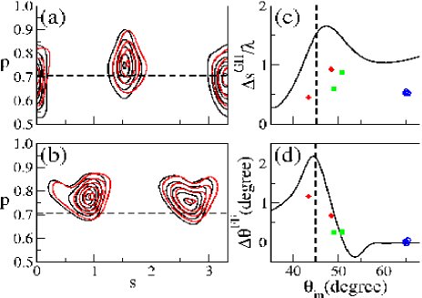
Figure 3: (color online) Contour plots of $H^{inc}(s,p)$(black line) and $H^{refl}(s,p)$(red line) for the diamond case (a) and the rectangle case (b). The Goos-Hänchen shifts (c) and the angular shifts (d) with the incident angle $\theta_{in}=\arcsin|p^{in\pm}|$. The solid diamonds and solid rectangles represent results of the corresponding scarred resonances. The open blue circles are for the hexagonally scarred resonance in Fig. 5 (a). The solid line is the result of a numerical calculation for a Gaussian incident beam at planar interfaceLa86 .

Note that the incident angles of the scarred patterns are always greater than the incident angles expected from the corresponding periodic ray orbits, i.e., $|p^{in\pm}_{i}|>p^{*}_{i}$. This means that the scarring pattern does not correspond to a simple connection of $s^{in\pm}_{i}$. In order to know the scar beam trajectories, we need to know positions of localized spots in the reflective Husimi function $H^{refl}(s,p)$. From the difference between $H^{inc}(s,p)$ and $H^{refl}(s,p)$, we can then estimate the Goos-Hänchen shiftsGo47 and angular shifts of the reflected beams, i.e., $(\Delta s^{GH\pm}_{i},\Delta p^{FF\pm}_{i})=(|s^{out\pm}_{i}-s^{in\pm}_{i}|,\pm(p^{out\pm}_{i}-p^{in\pm}_{i}))$. Since the angular shift $\Delta p^{FF}_{i}$ originates from the partial refractive escape from the microcavity, it can be interpreted as the Fresnel filtering effect on the reflected beam and expected to be reduced as the refractive escape decreases. In Fig. 3 (a) and (b) are shown the differences between $H^{inc}(s,p)$ and $H^{refl}(s,p)$ for both type-I scarred resonances. While the Goos-Hänchen shifts are clearly seen in both cases, the angular shift is evident only in the diamond case due to large refractive escape. The $\Delta s^{GH\pm}_{i}$ and $\Delta\theta^{FF}_{i}$ are plotted as a function of incident angle $\theta_{in}$ in Fig. 3 (c) and (d), respectively. The Goos-Hänchen shifts distribute around $0.5\lambda$, $\lambda=2\pi/k$, and the angular shifts decrease with increasing $\theta_{in}$. This result is qualitatively consistent with the numerical calculation(solid line) for a Gaussian beam incident on a planar interfaceLa86 .

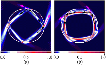
Figure 4: (color online) The positive chiral components in the type-I scarred resonance. (a) diamond case. (b) rectangle case. The arrows correspond to the peak positions $(s^{in,out+}_{i},p^{in,out+}_{i})$ of Husimi functions. Note that the patterns are slightly rotated from the symmetric periodic orbits. The negative chiral components are just the images of mirror reflection.

In Fig. 4 the arrows inside the microcavity correspond to the peak positions $(s^{in,out+}_{i},p^{in,out+}_{i})$ of both Husimi functions and the arrows for refractive escapes are obtained from the replacement of $P_{s}(s,p)$ by $H^{inc}(s,p)$ in Eq.(1). The background plots are the positive chiral components obtained by filtering the negative chiral components in the BEM. It is clearly shown that the internal patterns are slightly rotated in opposite directions in both type-I scarred resonances, and show a good agreement with the arrows. The same plots for the negative chiral components are just the mirror images of the positive ones. As a result, in the type-I scarred resonances the spatial splitting of two chiral components are clearly seen.

While the localized spots in $H^{inc}(s,p)$ of type-I scarred resonance are located near the critical line as shown in Fig. 2, in type-II the localized spots are far above the critical line, which means that type-II scarred resonances have much higher $Q$ factor due to strong confinement of light by total internal reflection and the refractive emission is very weak. In Fig. 5 (a) is shown an example of type-II scarred resonance showing a hexagonal scarring pattern which is drawn on logarithmic scale for visibility of the weak refractive emission beams. From this figure we can find a striking feature of the type-II scarred resonance that light emissions do not match with the scarring pattern inside the microcavity. In this hexagonal example, although the number of the bouncing points of the scarring pattern is six, the number of the emitting points is four. This mismatch between the scarring pattern inside and the emitting pattern outside is very important in practical experiments because the type-II scarred modes cannot be inferred from far field measurements.

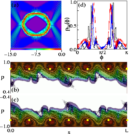
Figure 5: (color) (a) Type-II scarred resonance with $kR=(91.17,-0.0137)$ on logarithmic scale. (b) and (c) $H^{inc}(s,p)$ on logarithmic scale and the SPD structure. The yellow dots represent the periodic hexagonal orbit, $(s^{*}_{i},\pm p^{*}_{i})$. (d) Far field distributions. The histogram is the result of the SPD and the red line is for the type-II scarred resonance shown in (a), and the blue line is for another hexagonal scarred resonance with higher $k$, $kR=(170.58,-0.0117)$.

Although the $H^{inc}(s,p)$ of the hexagonal resonance simply shows, on the normal scale, six spots near the line of $p=\pm 0.90$, details near the critical line can be visible in logarithmic scale plot shown in Fig. 5 (b) and (c). Here, we emphasize that the structure of $H^{inc}(s,p)$ below the critical line resembles closely that of SPD. This implies that a few of rays consisting in the hexagonal scarring pattern diffuses chaotically and escapes below the critical line and this process happens on the structure of SPD. Note that the structure of SPD reveals the degree of the openness on the unstable manifold structure. Therefore, the SPD structure near the critical line is the major factor to determine the emission patterns of type-II scarred resonances.

The $P_{far}(\phi)$ based on the SPD structure in Eq.(1) is shown in Fig. 5 (d) as a histogram. This shows a good agreement with the far field distribution (red line) of the type-II resonance shown in Fig. 5 (a). We note that the ray dynamical analysis always corresponds to the limit of $k\rightarrow\infty$. The small discrepancy of emission angles would be therefore reduced as $k$ increases. The blue line in Fig. 5 (d) is the $P_{far}(\phi)$ of another hexagonally scarred resonance with higher $k$, and shows an improved agreement with the SPD result.

In conclusion, we describe the properties of scarred resonances in a chaotic microcavity. Their interesting behaviors have been explained in terms of the SPD in ray dynamics. The type-I scarred resonances are characterized by the correspondence between the scarring and the emission patterns and the spatial splitting of two chiral components. On the other hand, the characteristics of type-II scarred resonances are the mismatch of the emission pattern with the scarring pattern inside, and the unique emission pattern given by the SPD. The results would be very crucial to understand the directionality and internal patterns of scarred lasing modes generated from a chaotic microcavity in practical experiments.

We thank T. Harayama, Y.-H. Lee, S.-W. Kim, L. Xu, J. Wiersig for useful discussions during the NCRICCOC Workshop at Pai-Chai University. This work is supported by Creative Research Initiatives of the Korean Ministry of Science and Technology.

References

- (1)
- (2) Optical Processes in Microcavities, edited by R. K. Chang and A. J. Campillo (World Scientific, Singapore, 1996).
- (3) J. U. Nöckel and A. D. Stone, Nature 385, 45 (1997).
- (4) E. J. Heller, Phys. Rev. Lett. 53, 1515 (1984).
- (5) S.-B. Lee, J.-H. Lee, J.-S. Chang, H.-J. Moon, S. W. Kim, and K. An, Phys. Rev. Lett. 88, 033903 (2002); C. Gmachl, E. E. Narimanov, F. Capasso, J. N. Ballargeon, and A. Y. Cho, Opt. Lett. 27, 824 (2002); T. Harayama, T. Fukushima, P. Davis, P. O. Vaccaro, T. Miyasaka, T. Nishimura, and T. Aida, Phys. Rev. E 67, 015207(R) (2003).
- (6) N. B. Rex, H. E. Tureci, H. G. L. Schwefel, R. K. Chang, and A. D. Stone, Phys. Rev. Lett. 88, 094102 (2002).
- (7) S.-Y. Lee, S. Rim, J.-W. Ryu, T.-Y. Kwon, M. Choi, and C.-M. Kim, Phys. Rev. Lett. 93, 164102 (2004).
- (8) J. Hawkes and I. Latimer, Lasers; Theory and Practice (Prentice Hall, 1995).
- (9) A. Bäcker, S. Fürstberger, and R. Schubert, Phys. Rev. E 70, 036204 (2004).
- (10) M. Hentschel, H. Schomerus, and R. Schubert, Europhys. Lett. 62, 636 (2003).
- (11) J. Wiersig, J. Opt. A: Pure Appl. Opt. 5, 53 (2003).
- (12) S.-Y. Lee and S. C. Creagh, Ann. Phys. 307, 392 (2003).
- (13) F. Goos and H. Hänchen, Ann. Phys. (Leipzig) 1, 333 (1947); M. Hentschel and H. Schomerus, Phys. Rev. E 65, 045603(R) (2002).
- (14) We consider a sum of plane waves with a Gaussian angular distribution, , where and , for details see H. M. Lai, F. C. Cheng, and W. K. Tang, J. Opt. Soc. Am. A 3, 550 (1986).