Traveling Wave Fronts and Localized Traveling Wave Convection in Binary Fluid Mixtures

Abstract

Nonlinear fronts between spatially extended traveling wave convection (TW) and quiescent fluid and spatially localized traveling waves (LTWs) are investigated in quantitative detail in the bistable regime of binary fluid mixtures heated from below. A finite-difference method is used to solve the full hydrodynamic field equations in a vertical cross section of the layer perpendicular to the convection roll axes. Results are presented for ethanol-water parameters with several strongly negative separation ratios where TW solutions bifurcate subcritically. Fronts and LTWs are compared with each other and similarities and differences are elucidated. Phase propagation out of the quiescent fluid into the convective structure entails a unique selection of the latter while fronts and interfaces where the phase moves into the quiescent state behave differently. Interpretations of various experimental observations are suggested.

I INTRODUCTION

Many nonlinear dissipative systems that are driven sufficiently far away from thermal equilibrium show selforganization out of an unstructured state: A structured one can appear that is characterized by a (spatially extended) pattern which retains some of the symmetries of the system CH93 . Convection in binary miscible fluids like ethanol-water, ³He $-^{4}$He, or various gas mixtures is an example of such systems. It shows rich and interesting pattern formation behavior and it is paradigmatic for problems related to instabilities, bifurcations, and selforganization with complex spatiotemporal behavior.

Compared to convection in one-component fluids like, e.g., pure water the spatiotemporal properties are far more complex. The reason is that concentration variations which are generated via thermodiffusion, i.e., the Soret effect by externally imposed and by internal temperature gradients influence the buoyancy, i.e., the driving force for convective flow. The latter in turn mixes by advectively redistributing concentration. This nonlinear advection gets in developed convective flow typically much larger than the smoothening by linear diffusion — Péclet numbers measuring the strength of advective concentration transport relative to diffusion are easily $\cal O$(1000). Thus, the concentration balance is strongly nonlinear giving rise to strong variations of the concentration field and to boundary layer behavior. In contrast to that, momentum and heat balances remain weakly nonlinear close to onset as in pure fluids implying only smooth and basically harmonic variations of velocity and temperature fields as of the critical modes.

Without the thermodiffusive Soret coupling between temperature and concentration any initial concentration deviation from the mean diffuses away and influences no longer the balances of the other fields. Hence, the feedback interplay between (i) the Soret generated concentration variations, (ii) the resulting modified buoyancy, and (iii) the strongly nonlinear advective transport and mixing causes binary mixture convection to be rather complex with respect to its spatiotemporal properties and its bifurcation behavior. Take for example the case of negative Soret coupling, $\psi<0$, between temperature and concentration fields coupling when the lighter component migrates to the colder regions thereby stabilizing the density stratification in the quiescent, laterally homogeneous conductive fluid state. Then the above described feedback interplay generates oscillations. In fact the buoyancy difference in regions with different concentrations was identified already in WKPS85 as the cause for traveling wave convection.

Oscillatory convection appears in the form of the transient growth of convection at supercritical heating, in spatially extended nonlinear traveling wave (TW) and standing wave solutions that branch in general subcritically out of the conductive state via a common Hopf bifurcation, in spatially localized traveling wave (LTW) states, and in various types of fronts. TW and LTW convection has been studied experimentally and theoretically for some time CH93 ; Moses87Heinrichs87 ; Behringer9091 ; Winkler92 ; Kolodner94 ; Platten96 ; Kaplan94 ; Surko91 ; Aegert01 ; Ning97b ; Batiste01 ; Jung02 . The transient oscillatory growth of convection was investigated by numerical simulations FL . Nonlinear standing wave solutions were obtained only recently MJL04 ; JML04 . Freely propagating convection fronts that connect subcritically bifurcating nonlinear TW convection with the stable quiescent fluid do not seem to have been investigated in detail beyond some first preliminary results Bensimon90 ; Kolodner92Fronts ; Bu99 . Here we determine such fronts in quantitative detail and compare their properties with those of LTWs.

In narrow rectangular and annular channels convection occurs in the form of rolls with axes oriented perpendicular to the long sidewalls Surko87 ; CH93 . These stuctures can efficiently be described in the two dimensional vertical $x-z$ cross section in the middle of the channel perpendicular to the roll axes ignoring variations in axis direction. Furthermore, these convection structures have relevant phase gradients only in $x$-direction thus causing effectively one dimensional patterns AlBa04 .

When comparing experiments with analytical calculations or numerical simulations performed under the above described conditions it is useful to do that on the basis of reduced Rayleigh numbers, $r=R/R^{0}_{c}$, with $R^{0}_{c}$ being the critical one for onset of pure fluid convection for the respective experiment, analytical method, or numerical method. This significantly reduces the dependence of, say, the bifurcation diagrams of convective states on the specific geometry of the respective set-up. In laterally unbounded systems the analytical value for $R^{0}_{c}$ is 1707.762.

Localized traveling waves.     For weak negative Soret coupling one has observed in experiments a competition between homogeneous laterally extended TW convection and so-called dispersive chaos with an irregular repetitive formation and collapse of spatially localized TW pulses Kolodner90Glazier91 ; Kaplan94 . During the pulse formation their drift velocities can drop abruptly to about a tenth of the initial group velocity Kolodner90Glazier91 . We consider this to be a characteristic signal that the lateral redistribution of concentration over the pulse Jung02 becomes important and that the strongly nonlinear dynamics sets in. For more negative $\psi\lesssim-0.06$ the collapse is in general less dramatic. There, convection is dominated by isolated strongly peaked localized states. Eventually, at $\psi\simeq-0.07$ a regime is reached where stable LTWs coexist near onset with extended TWs Barten95I ; Barten95II ; Luecke98 ; Moses87Heinrichs87 ; Kolodner88 ; Kolodner91a ; Kolodner94 . Increasing the Soret coupling strength further to more negative $\psi$ the band ($r^{LTW}_{min},r^{LTW}_{max}$) of Rayleigh numbers in which stable LTWs exist increases monotonically while shifting upwards as a whole — $r^{LTW}_{max}(\psi)$ grows stronger than $r^{LTW}_{min}(\psi)$. Simultaneosly, the lower band limit for the existence of extended TW states $r^{TW}_{min}(\psi)$, i.e., the lowest saddle-node of TWs increases even steeper so that eventually for $\psi\lesssim-0.4$ the complete LTW band comes to lie below the existence range of TWs, $r^{LTW}_{max}\leq r^{TW}_{min}$ Jung02 .

LTWs consist of slowly drifting, spatially confined convective regions that are embedded in the quiescent fluid. These intriguing structures have been investigated in experiments Moses87Heinrichs87 ; Kolodner88 ; Bensimon90 ; Niemela90 ; Behringer9091 ; Kolodner9091 ; Steinberg91 ; Kolodner91a ; Surko91 ; Kolodner91c ; Kolodner91d ; Kolodner93II ; Kolodner94 and numerical simulations Barten91 ; Barten95II ; Luecke98 ; Jung02 . A discussion of various theoretical models aiming at their explanation is contained in Sec. III.5. Roll vortices grow in a LTW structure out of the quiescent fluid at one end, travel with spatially varying phase velocity $v_{p}(x)$ to the other end, and decay there back into the basic state. The two interfaces to conduction and with it the whole convective region move with constant, uniquely selected drift velocity $v_{d}$. The latter is a function of $r,\psi$ with magnitude much smaller than the phase velocities. Also the oscillation frequency of the LTW is uniquely selected; it is constant in space and time in the frame that is comoving with its drift velocity. And finally, the length $l(r,\psi)$ of the convective region of stable LTWs and their spatial stucture are uniquely selected. This length grows with increasing heating $r$.

A central role for the stable existence of LTWs plays a large-scale mean concentration current. Extending over the whole LTW it redistributes concentration and thereby changes the buoyancy in a decisive way Luecke98 . This effect can sustain LTWs even at low $r$ where no extended TWs exist Jung02 .

Blinking states in rectangular channels.     The LTW confinement of convection occurring in translationally invariant annular channels is obviously an inherent process of the hydrodynamic balances. But one has also observed end-wall-assisted or at least end-wall-modified confinement of convection close to the ends of rectangular channels. The weakly nonlinear varieties of such a confinement can largely be understood in terms of the convective behavior of TW packets, their reflection properties at the end walls, and the destructive interaction between left and right traveling patterns Cross868889 ; Brand86 ; Fineberg90 . These effects give rise near onset to a wide range of weakly nonlinear and effectively low dimensional spatiotemporal behavior that depends sensitively on the specific experimental set-up like, e.g., the end-wall boundary conditions and the system length Kolodner8889 ; Fineberg88Steinberg89 ; Bestehorn89 ; Kolodner93 ; Batiste01 . While the linear eigenmodes of such sytems (’linear counterpropagating waves’ or ’chevrons’) Kolodner86 ; Surko87 ; Kolodner87 ; Batiste01 are laterally symmetric or antisymmetric localization sets in via a temporal amplitude modulation. Thereby convection is alternatingly weakened and enhanced in the left and the right part of the system part giving rise to a ’blinking’ state Surko87 ; Kolodner8889 ; Fineberg88Steinberg89 ; Steinberg91 ; Kolodner93 . The so-called ’chaotic blinking’ states Kolodner8889 ; Fineberg88Steinberg89 ; Steinberg91 ; Kolodner93 seem to be the analogue of the ’chaotic dispersive’ pulse formation in annular containers Steinberg91 ; Kaplan94 . Also ’blinking’ modes with different frequencies at both ends of the channel were observed Fineberg88Steinberg89 ; Steinberg91 . But their possible relation to a large-scale mean concentration variation Moses86 produced by nonlinear propagating waves in a finite cell has not been discussed.

Wall-attached structures.     At larger $r$ one has observed wall-attached TW structures with amplitudes confined to the vicinity of one or both end walls. These wall-attached convective patches Moses87Heinrichs87 ; Kolodner8889 ; Fineberg88Steinberg89 ; Kolodner90 ; Kolodner91b ; Yahata91 ; Ning96 ; Ning97a are closely related to free LTWs Niemela90 . They are strongly nonlinear as indicated by their low frequency Kolodner8889 ; Fineberg88Steinberg89 . Moreover, their spatial structure and their region of existence is largely unaffected by the details of the lateral boundaries or by the container length in contrast to the linear and weakly nonlinear behavior described above Fineberg88Steinberg89 . The more extensive wall-attached structures show some similarities with front-like states. Note, however, that here the source or the sink of the propagating rolls is pinned near a wall and the interface to the quiescent fluid in the bulk of the channel does not move Kolodner90 .

Our numerical simulations.     Our numerical simulations have been performed in order to elucidate in quantitative detail the properties of relaxed nonlinear TW convection structures that contain an interface (or two of them) to the quiescent fluid as an integrated structural element. We compare for a wide range of Soret coupling strengths front states and LTW states showing what they have in common and how they differ. We focus our interest to those parameters where the quiescent conductive state of the fluid is stable and where the solutions describing spatially extended, laterally periodic TW convection bifurcate subcritically out of it.

The system we have in mind is a binary fluid layer of thickness $d$ which is bounded by two solid horizontal plates perpendicular to the gravitational acceleration ${\bf g}$. The fluid might be a mixture of water with the lighter component ethanol at a mean concentration $\overline{C}$. It is heated from below. The temperatures at the plates are $\overline{T}\pm\Delta T/2$. The variation of the fluid density $\rho$ due to temperature and concentration variations is governed by the linear thermal and solutal expansion coefficients $\alpha=-\frac{1}{\rho}\frac{\partial\rho}{\partial{T}}$ and $\beta=-\frac{1}{\rho}\frac{\partial\rho}{\partial{C}}$, respectively. Both are positive for ethanol-water. The solutal diffusivity of the binary mixture is $D$, its thermal diffusivity is $\kappa$, and its viscosity is $\nu$. Length and time is scaled by $d$ and $d^{2}/\kappa$, respectively, so that velocity is measured in units of $\kappa/d$. Temperatures are reduced by the vertical temperature difference $\Delta T$ across the layer and concentrations by $\frac{\alpha}{\beta}\Delta T$. The scale for the pressure is given by $\frac{\rho\kappa^{2}}{d^{2}}$.

Then, the balance equations for mass, momentum, heat, and concentration LL66 ; Platten84 read in Oberbeck–Boussinesq approximation Barten95I

$$\mbox{\bf\boldmath$\nabla$}\cdot{\bf u}=0$$ (1a)

$$\partial_{t}\,{\bf u}=-{\bf\mbox{\boldmath$\nabla$}}\,({\bf u:u}+p-\sigma\,{\bf\mbox{\boldmath$\nabla:$}\,\,u})+{\bf B}\,\,\,;\,\,\,{\bf B}=\sigma\,R\,(\delta T+\delta C){\bf e}_{z}$$ (1b)

$$\partial_{t}\delta T=-\mbox{\bf\boldmath$\nabla$}\cdot\left[{\bf u}\delta T-\mbox{\bf\boldmath$\nabla$}\delta T\right]$$ (1c)

$$\partial_{t}\delta C=-\mbox{\bf\boldmath$\nabla$}\cdot\left[{\bf u}\delta C-L\mbox{\bf\boldmath$\nabla$}\left(\delta C-\psi\delta T\right)\right]\ .$$ (1d)

Here, $\delta T$ and $\delta C$ denote deviations of the temperature and concentration fields, respectively, from their mean $\overline{T}$ and $\overline{C}$ and $\bf B$ is the buoyancy. The Dufour effect HLL92 ; HL95 that provides a coupling of concentration gradients into the heat current and a change of the thermal diffusivity is discarded in (1c) since it is relevant only in few binary gas mixtures LA96 and possibly in liquids near the liquid–vapor critical point LLT83 .

Besides the Rayleigh number $R=\frac{\alpha gd^{3}}{\nu\kappa}\Delta T$ measuring the thermal driving of the fluid three additional numbers enter into the field equations: the Prandtl number $\sigma=\nu/\kappa$, the Lewis number $L=D/\kappa$, and the separation ratio $\psi=-\frac{\beta}{\alpha}\frac{k_{T}}{\overline{T}}=-S_{T}\overline{C}(1-\overline{C})\frac{\beta}{\alpha}$. Here $k_{T}=\overline{T}\,\overline{C}(1-\overline{C})S_{T}$ is the thermodiffusion coefficient LL66 and $S_{T}$ the Soret coefficient. They measure changes of concentration fluctuations due to temperature gradients in the fluid. $\psi$ characterizes the sign and the strength of the Soret effect. Negative Soret coupling $\psi$ (i.e., positive $S_{T}$ for mixtures like ethanol water with positive $\alpha$ and $\beta$) induces concentration gradients of the lighter component that are antiparallel to temperature gradients. In this situation, the buoyancy induced by solutal changes in density is opposed to the thermal buoyancy.

When the gradient of the total buoyancy exceeds a threshold, convection sets in — typically in the form of straight rolls. For sufficiently negative $\psi$ the primary instability is oscillatory. Ignoring field variations along the roll axes we describe here 2D convection in an $x$–$z$ plane perpendicular to the roll axes with a velocity field

$${\bf u}(x,z,t)=u(x,z,t)\,{\bf e}_{x}+w(x,z,t)\,{\bf e}_{z}\,.$$ (2)

To find the time-dependent solutions of the above partial differential equations subject to realistic horizontal boundary conditions Barten95I we performed numerical simulations with a modification of the SOLA code that is based on the MAC method MAC-SOLA ; PT83 . This is a finite-difference method of second order in space formulated on staggered grids for the different fields. The Poisson equation for the pressure field that results from taking the divergence of (1b) was solved iteratively with the artificial compressibility method PT83 by incorporating a multi-grid technique.

Throughout this paper we consider mixtures with $L=0.01$, $\sigma=10$, and various negative values of $\psi$ that are easily accessible with ethanol-water experiments. The paper is organized as follows: In Sec. II we first describe our methods for characterizing the various convective states. Then we present results for the two different types of TW front states that can arise in laterally homogeneous mirror symmetric systems with either the phase propagating out of the quiescent fluid or into it. Also transient two-front structures are discussed. Sec. III deals with LTW states and their relation to fronts. The transient dynamics towards the selected LTW, the stabilization via front repulsion, the difference between long and short LTWs, and a critical appraisal of LTW models are topics covered here. In Sec. IV we present a comparison with experiments and a discussion. The last section contains a conclusion.

II Fronts

Here we discuss front solutions where part of the system is occupied by the quiescent fluid while the other one shows fully developed, saturated, strongly nonlinear TW convection with laterally homogeneous amplitude. Strictly speaking these two states are realized only in the two opposing limits of $x\to\pm\infty$. We focus our investigation of fronts on parameters where the quiescent fluid state is stable and where the TW solutions bifurcate subcritically out of the conductive state. Then, any linear growing and spreading of infinitesimal, localized convective perturbations in the quiescent fluid which could possibly dominate the low amplitude behavior of fronts as in the case of an unstable zero amplitude state vSaarloos9092 ; vSaarloos03 is absent.

Little general is known about pattern forming fronts in real bistable systems CH93 . Most of the research activities were centered on fronts in the quintic Ginzburg-Landau equation vSaarloos9092 ; vHvSHo93 ; CoWaSMi99 ; CoCh01 ; SzLu03 ; Rabaud03 . One can expect that the front properties are fixed by a strongly nonlinear eigenvalue problem describing a heteroclinic orbit between the two involved states. Some of these front solutions will be unstable. There might be also multistable coexistence of fronts so that depending on initial conditions and on the history of the (control) parameters different fronts could finally be realized. We call a front uniquely selected when our numerical simulations indicated that different formation processes ended in the same front for a fixed parameter combination.

Fronts can be classified into coherent and incoherent ones vSaarloos03 . We focus here on the first kind which in our system are characterized as strictly time periodic states in a frame that is comoving with the front’s velocity $v_{F}$. Such a front state being monochromatic is a global nonlinear mode. Its frequency is an eigenvalue, i.e., a global constant in space and time so that the convection oscillations have everywhere the same period.

Thus, we do not consider here, e.g., complex large scale or chaotic spatiotemporal interface behavior. The coherent fronts of the various hydrodynamic fields and quantities in this paper have a smooth and basically monotonous profile which connects the quiescent fluid with the nonlinear saturated extended TW. The transition region between conduction and convection that is characterized by large amplitude variations is quite short and consists typically only of about 3 -4 convection rolls. We call this transition region also the interface between conduction and convection.

If the selected front pattern is incompatible with any stable bulk structure there are two possibilities: (i) A perturbation in the unstable convection bulk grows and expands towards the interface. This would destroy front coherence and could lead to more complex large scale variations, perhaps chaotic spatiotemporal behavior. (ii) The interface region is only convectively unstable against perturbations of the bulk nonlinear TW. Then initially localized perturbations would be advected out of every finite system and could not reach the unperturbed interface region of the front.

II.1 Methods of characterization

II.1.1 Definitions

We call a front to be of type $+$ when its envelope grows at $x=-\infty$ out of the basic quiescent state. Otherwise it is a $-$front. Then the amplitude falls to zero at $x=+\infty$ Buechel00 . The phase of the convection pattern in a front state of type $+$ can either propagate to the left or to the right and similarly for the $-$front state. Hence, one would have to discuss four front states separately. However, because of the invariance of the system under $x\to-x$ a $+$front state with positive (negative) phase velocity $v_{p}$ is the mirror image of the $-$front state with negative (positive) $v_{p}$. Therefore, it suffices to consider only the front states that consist of roll vortices traveling, say, in positive $x$-direction and to use the superscript $+$ or $-$ to identify the properties of the front in question in a unique way. So, the phase velocities of all oscillatory convective structures investigated in this paper are positive. We call the direction of positive $x$ into which the phase propagates also ’downstream’ and the opposite one ’upstream’.

So, to sum up our notation: In a $+$front state the quiescent fluid is located ’upstream’ and a source of phase with the latter propagating out of the conductive state into convection. In a $-$front the quiescent fluid is located in ’downstream’ direction and a sink since phase moves out of convection into conduction.

Fig. 1 shows fronts of each type. Under the $+$front (left half of Fig. 1) convection rolls grow out of the quiescent fluid and saturate in a ’downstream’ bulk TW. On the other hand, a $-$front (right half of Fig. 1) annihilates roll vortices. In this process their phase velocity is accelerated [cf. the increase in the lateral profile of $v_{p}(x)$ in Fig. 1(f)] and they are stretched horizontally.

It is clear from Fig. 1 that the quiescent (convecting) region expands into the convecting (quiescent) one when the velocity $v^{+}_{F}$ of the $+$front is positive (negative) and vice versa for the $-$front.

II.1.2 Mixing number

In order to monitor how well the fluid is mixed along the front we always determined for the relaxed front states the mixing number

$$M(x)=\left[<\overline{(\delta C)^{2}}>/\overline{(\delta C_{cond})^{2}}\right]^{1/2}$$ (3)

as a function of lateral position $x$. It basically measures the mean square of the deviations $\delta C(x,z,t)$ of the concentration field from its global mean: the overbars imply a vertical average and the brackets a temporal average at the specific horizontal location $x$ in the frame comoving with the front velocity $v_{F}$. The subscript cond denotes the reference quiescent conductive state with its linear vertical concentation variation. The mixing number is defined such that $M=0$ in a perfectly mixed fluid and $M=1$ in the quiescent state.

In laterally extended TWs $\omega$ and with it $v_{p}$ increase when the concentration variations become larger Barten95I ; Luecke98 . In fact, there is a universal scaling relation between $M$ and $\omega$ HoBuLu97 which shows that $M$ and $v_{p}$ are linearly related to each other. This relation also holds for the bulk part of front states far away from the interface where the convection is TW-like with only slow spatial amplitude variation (Fig. 1).

II.1.3 Concentration current

The phase shift between the concentration and velocity waves in the TW-like bulk of the front states sustains as in extended TW states a mean lateral concentration current $<{\bf J}>(x,z)$ Linz88 ; Barten89 ; Barten95I ; Luecke98 :

$$<{\bf J}>=<{\bf u}\delta C-L\mbox{\bf\boldmath$\nabla$}(\delta C-\psi\delta T)>$$ (4)

where ${\bf u}$ is the velocity field and $\delta T$ the temperature deviation from the global mean. Again, the brackets imply a temporal average in the frame that is comoving with the front velocity. The Lewis number $L=0.01$ being rather small in our simulations implies that $<{\bf J}>$ is dominated by the advective contribution except in those boundary regions in which ${\bf u}$ becomes small.

The vertical variation of $<{\bf J}>$ is such that positive (negative) $\delta C$ is transported in phase direction in the upper (lower) half of the layer. This transport causes a large-scale concentration redistribution in a front state between its TW bulk and its interface to the quiescent fluid and it is responsible for the different characteristic structures of the interfaces in a $+$ and a $-$front as we will see further below.

II.1.4 Preparation and lateral boundary conditions

We simulated systems containing up to 160 rolls. The initial state was prepared by filling one half of the sytem with a nonlinear TW that was previously generated with periodic boundaries to have some fixed wavelength $\lambda$. The other half contained the stable temperature and concentration distribution of the pure quiescent basic state.

To simulate $+$fronts in infinite systems that connect to developed TW convection with some wavelength $\lambda$ far away from the interface between conduction and convection we imposed at the ’downstream’ boundary $x=L$ of our computation domain the periodicity condition $f(L)=f(L-\lambda)$. For the case of $-$fronts we found that imposing the analogous condition at the ’upstream’ boundary of the developed TW part at $x=-L$ typically will introduce perturbations that can grow in ’downstream’ direction for example when the TW region is Eckhaus unstable. The different aspects of the stability of $+$ and $-$fronts are discussed further below in the paper.

After a relaxation time of typically 100 to 200 vertical thermal diffusion times we then could observe under certain conditions a coherent front state connecting a quiescent region of the system to a TW with asymptotic wavelength $\lambda$. Here the fact that the frequency $\omega$ of such a coherent front state is constant in space and time in the frame that is comoving with the front velocity $v_{F}$ proved to be a good relaxation criterion to effectively determine whether such a state had been obtained.

II.2 $+$Fronts

II.2.1 Structure and dynamics

As soon as the growing convection rolls in a $+$front have become sufficiently nonlinear, i.e., when their lateral flow velocity $u$ has grown up to about their phase velocity $v_{p}$ [e.g., close to the vertical arrow in Fig. 1(c)] they start to alternatingly suck in positive (’blue’) and negative (’red’) $\delta C$ from the top and bottom concentration boundary layers, respectively. It is transported away into the well mixing convection bulk and replaced at the interface location by neutral (’yellow/green’) $\delta C$. Note that increasing $u$ beyond $v_{p}$ causes the appearence of closed streamlines of the velocity field in the frame comoving with the phase velocity of a traveling roll Linz88 ; Luecke98 ; JML04 . These closed streamlines regions are responsible for the characteristic roll structure of the $C$ field in Fig. 1(a): Positive (negative) $\delta C$ is collected from the top (bottom) boundary layers and transported within the homogeneously mixed closed streamline regions in phase direction while mean concentration, $\delta C\simeq 0$, is advected along the meandering ”green-yellow stripe” in Fig. 1(a) to the left Jung02 . The mean concentration current $<{\bf J}>$ resulting from this complicated concentration redistribution is shown in Fig. 1(i). All in all, mean concentration is accumulated (depleted) at the $+$ ($-$) front interface.

The concentration redistribution reduces at the interface of the $+$front the Soret-induced solutal stabilization that occurs to the left of it as a result of the large conductive vertical concentration gradient: at the interface one can observe a minimal mixing number [Fig. 1(e)] and with it a buoyancy overshoot [Fig. 1(g)] which is sufficiently large to sustain local convection growth there and cause even invasion of convection into the quiescent region whenever $v_{F}^{+}<0$. With the fluid being well mixed there, i.e., with $M$ being small the local phase velocity is also small there – in fact the minimum of $v_{p}(x)$ in Fig. 1(e) lies close to the one in $M$.

Since the strongly stable quiescent fluid to the left of the $+$front prohibits a well developed advectively mixing front tail the reduction of $\delta C$ variations there is driven primarily by diffusion. The latter having a characteristic time scale given by $L=0.01$ explains why the front velocities are much smaller than the fast phase velocity.

When $r$ is increased $v_{F}^{+}$ tends to become (more) negative: convection to the right of the $+$interface can now, with increased heating, better invade the quiescent fluid to the left of it and thus $\partial_{r}v_{F}^{+}(r,\psi)<0$. Similarly, when $\psi$ is increased, i.e., when the convection suppressing Soret effect is diminished the expansion of TW convection is favoured and thus $\partial_{\psi}v_{F}^{+}(r,\psi)<0$.

Moving along the $+$front in Fig. 1 to the right from the interface towards the asymptotic TW state at large $x$ there develops an equilibrium between the $\delta C$ feed-in from the boundary layers at the plates and the amount of advective mixing: The concentration contrast between two neighboring rolls increases on the way towards the TW bulk. With it the phase speed $v_{p}(x)$, the wavelength $\lambda(x)=2\pi v_{p}(x)/\omega$, and the lateral concentration current $<{\bf J}>$ grow monotonously up to their asymptotic TW values. This growth extends laterally over a wide interval which itself increases when the Soret coupling becomes stronger.

We found that the minimal wavelength in a $+$front state is located at the interface and – more remarkably – that it is about $\lambda_{min}\sim 1.4$ for all $r$ and $\psi$ that we have simulated. We have no real quantitative explanation for this strong universal selection of the local wavelength at the interface. Intuitively the growing rolls are squeezed in the region with the negative lateral gradient of $M$. The squeezing is relaxed when the rolls begin to absorb high concentration contrasts from the plate layers which increases $v_{p}$ again [arrow in Fig. 1(c)].

It is interesting to note that the mean concentration current $<{\bf J}>$ of TWs becomes maximal close to the TW saddle node, i.e., where the asymptotic TW parts of our front states are located. Finally we mention that the front states do not sustain a measurable lateral meanflow; the quiescent fluid prohibits that. On the other hand, extended TWs in laterally periodic systems show in general a Reynolds stress-induced meanflow of the order $10^{-3}$ Linz88 ; Barten95I ; Luecke98 . But it goes through zero just near the TW saddle node.

II.2.2 Bifurcation properties

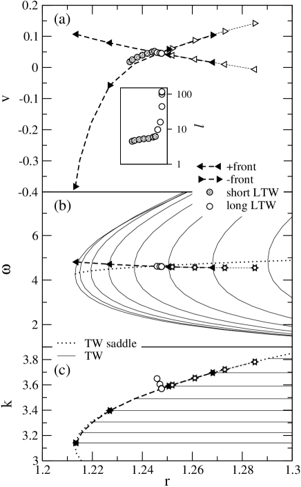
Figure 2: Front and LTW bifurcation properties versus reduced Rayleigh number $r=R/R^{0}_{c}$ for $\psi=-0.25$. Left and right pointing triangles with triangles denote $+$ and $-$fronts, respectively. Open and shaded circles refer to long and short LTWs, respectively. (a) Front velocities of relaxed single-front states (thick dashed lines with filled triangles), of expanding two-front states (thin dashed lines with open triangles), and drift velocities of LTWs (circles). The inset shows the drastic increase of LTW length $l$ at $r^{LTW}_{\infty}=r^{F}_{eq}$ where the front velocities of the $+$ and $-$ single-front states become equal. (b) Frequencies of front states and of long LTWs in comparison with the rest frame frequencies of laterally periodic TWs. The saddle-node vicinities of the latter are shown by full lines for several wave numbers $k=2\pi/\lambda$. TW states with frequencies above the dotted line of saddle-node TWs are unstable. (c) Wave numbers selected by front states in the bulk part far away from the interface (triangles) and in the central part of long LTWs (open circles). Horizontal lines indicate the laterally periodic TWs that are shown in (b) by full lines. The continuum of these TW states is bounded in the $r-k$ plane by the dotted line of TW saddle nodes, $k_{s}^{TW}(r)$. Here we show only the large-$k$ branch of it (cf. the dotted line marked $r_{s}^{TW}$ in Fig. 5 for another perspective).

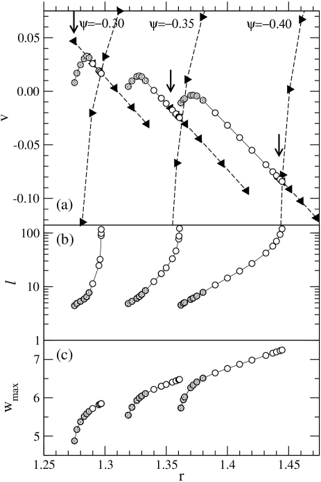
Figure 3: Front states and LTWs for different $\psi$. (a) Front velocities, $v_{F}$, of $+$fronts (left pointing triangles), of $-$ fronts (right pointing triangles), and drift velocities, $v_{d}$, of LTWs (circles) versus $r$. Note that short LTWs (shaded circles) and long LTWs (open circles) show different $v_{d}(r)$-behavior. The latter varying linearly with $r$ is nearly indistinguishable from $v^{+}_{F}(r)$. Arrows mark the low-$r$ existence boundary $r_{min}^{TW}$ of laterally periodic TWs and with it of front states. LTWs exist below this threshold Jung02 with drift velocities that show the above mentioned linear variation with $r$ as long as the LTWs are long enough. To identify an LTW as a long one we required a clearly visible plateau in the spatial properties. (b) Length $l$ of the LTWs of (a) measured as the distance between the half maximum values of the envelope of the vertical velocity field $w$ [cf., blue line in Fig. 1(c,d)]. (c) Maximal vertical flow velocities $w_{max}$ of LTWs.

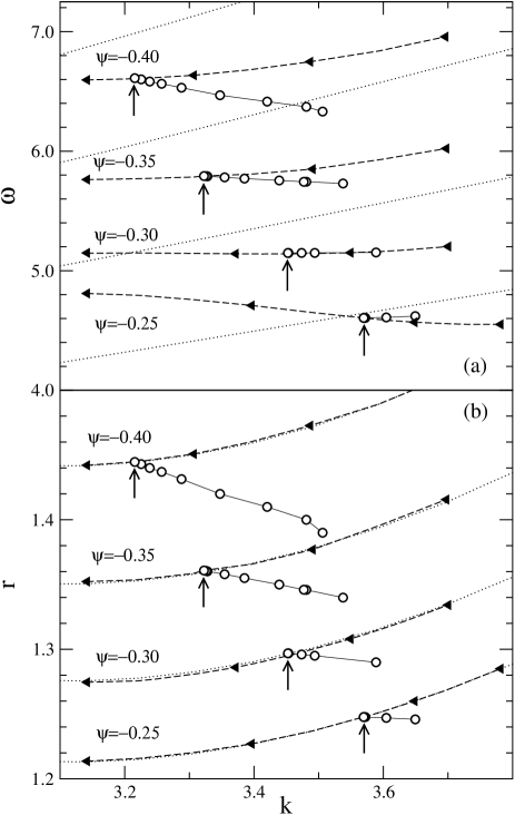
Figure 4: Wave properties of $+$fronts (dashed lines with triangles), long LTWs (circles), and laterally extended saddle-node TWs (dotted lines) for different $\psi$. The wave numbers of the two former refer to plateau values in the bulk part away from the interface. (a) Frequency $\omega$ (for TWs in the rest frame and for LTWs and fronts in the comoving frame) versus wave number $k$. (b) The same convection structures in the $k-r$ plane. The wave numbers and frequencies of LTWs with $l\to\infty$ (arrows) coincide at $r^{LTW}_{\infty}=r^{F}_{eq}$ with those of the respective $+$ fronts.

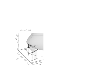
Figure 5: Laterally periodic TWs, $+$fronts, and LTWs in the three dimensional $k-r-\omega$ parameter space. Grey, nose-shaped surface Jung02 denotes TWs. They are unstable when $\omega$ is above the dotted line of saddle nodes. Its projection onto the $k-r$ is marked by $r^{TW}_{s}(k)$. A particular bifurcation branch for a given $k$ (e.g., the long-dashed line for $k\sim\pi$) starts backwards with a large Hopf frequency (not shown) and becomes stable by a saddle-node bifurcation at the dotted line. The big plus signs on the TW surface mark asymptotic $+$fronts. The small plusses at large $k$ denote the highest wave numbers occurring at the $+$front interface. Long LTWs are represented with their plateau values by big bullets. They coexist with fronts (big plusses) in a very narrow $r$ interval at $r^{LTW}_{\infty}$ close to the tip of the TW nose. The small bullets at large $k$ denote the largest local wave numbers occurring at the interface of convection growth. Each horizontal line indicates at fixed $r$ and $\omega$ the spatial variation of the local wave number $k$ within a $+$front or a long LTW from the growth interface to the asymptotic plateau value. The $k$ variation of LTWs from plateau to the decay interface into conduction is not shown.

In Figs. 2 - 5 we show the bifurcation properties of fronts in comparison with LTWs and laterally periodic TW states. We use front velocities and frequencies being temporally and spatially constant as order parameters to characterize all of the aforementioned oscillatory states. In addition we also consider the local wave numbers of front states and of LTWs in the bulk spatial regions where $\lambda(x)$ has reached a plateau, i.e., sufficiently away from any interface to conduction.

Figs. 2 and 3 show that the front velocities of $+$ and $-$fronts vary quite differently as a function of $r$. The former decrease linearly with growing $r$ and the latter increase, albeit not linearly. Thus, there is a crossing at $r^{F}_{eq}$ where $v_{F}^{+}$ becomes equal to $v_{F}^{-}$, so that both fronts move with the same velocity. At this Rayleigh number the length $l$ of the LTWs diverges, i.e., $r^{LTW}_{\infty}=r^{F}_{eq}$. There, and strictly speaking only there, this limiting LTW can be seen as a state consisting of two fronts.

The frequency and bulk wave number selected by a $+$front and of a very long LTW are close to those of the respective, laterally extended saddle-node TW (Figs. 2, 4, 5). A somewhat hand-waving explanation for the selection of the saddle-node frequency is as follows: With (i) convection growing out of conduction in a $+$ front, with (ii) small-amplitude extended TW perturbations of the latter oscillating according to a purely linear balance with the large Hopf frequency, and with (iii) the tendency to decrease $\omega$ with growing convection amplitude the saddle-node frequency is the first, i.e., the largest possible eigenfrequency of the full nonlinear front problem to allow for a stable TW region away from the interface.

A stable front state that has a TW bulk part extending laterally to infinity with frequency $\omega$ and wave number $k$ cannot be realized at $r$-values that lie below the saddle-node curve of laterally extended TWs, cf. the curve marked $r_{s}^{TW}$ in the $k-r$ plane of Fig. 5. Thus, the lowest Rayleigh number $r^{F}_{min}$ for the existence of fronts is $r_{min}^{TW}=r_{s}^{TW}(k\simeq\pi)$, i.e., the location of the tip of the nose-shaped TW bifurcation surface like the grey surface in Fig. 5. Ahead of this nose one cannot realize front states because at such locations there are no TWs to which the interface from conduction could connect.

The TW bulk parts of our $+$fronts are practically saddle-node TWs that have bulk wave numbers on the saddle-node curve $r_{s}^{TW}(k)$. Furthermore, it is interesting to note that they are on the large-$k$ branch of $r_{s}^{TW}(k)$ — the big plusses in Fig. 5 marking the bulk values of the front states lie all above $k\simeq\pi$. In fact, in all our simulations we did not find front states with bulk wave numbers smaller than $\pi$. This value marks for all $\psi$ that we investigated the tip of the nose-shaped TW bifurcation surface like the grey surface in Fig. 5.

In contrast to fronts, however, LTWs of finite length $l$ can coexist bistably together with the conductive state at $r$-values well below $r_{s}^{TW}(k)$: They can sustain over a finite lateral length convection with frequencies and bulk wave numbers (big bullets in Fig. 5) ”ahead” of the grey TW surface for reasons that are explained in Ref. Jung02 . This also shows that fronts and LTWs are quite different states. In the limit $l\to\infty$ the LTW states merge at $r^{LTW}_{\infty}=r^{F}_{eq}$ with a TW whose wave number and frequency is close to the TW saddle-node as shown in Figs. 2, 4, 5. Therefore, $\omega(r^{LTW}_{\infty})$ increases when the Soret coupling becomes more negative but $k(r^{LTW}_{\infty})$ decreases. For $\psi\lesssim-0.4$ it moves towards the tip of the TW nose at $k\simeq\pi$.

II.2.3 Front selection and stability

Simulations of $+$fronts that were done at fixed control parameters $r,\psi$ with different initial conditions, e.g., different wave numbers of an initial TW part produced in general a uniquely selected final front state with the same frequency and the same asymptotic bulk TW part. During the formation process initial wave structures with the ’wrong’ wave patterns propagated out of the system in the direction of the phase velocity and were substituted by convection that was selected by the front. That also explains why our TW boundary condition $f(L)=f(L-\lambda)$ at the ’downstream’ end has no measurable influence on the $+$front state even when $\lambda$ differs from the front-selected value.

The substitution dynamics is documented in Fig. 6. There a TW bulk part was prepared initially at $x>8$ with a wavelength of $\lambda=1.85$ and phase velocity $v_{p}=1.032$. The spatial region to the right of the interface to conduction is then invaded by the front-selected TW pattern that has a smaller bulk wavelength of $\lambda=1.80$ and that propagates with a faster phase velocity of $v_{p}=1.258$. The wave number is increased via several phase annihilating defects.

All our $+$interfaces selected bulk TW wave numbers close to the large-$k$ branch of the TW saddle-node curve; cf. Figs. 4(b) and 5 for $r^{TW}_{s}(k)$ and Fig. 2(c) for $k^{TW}_{s}(r)$. Thus, these wave numbers are too large to be Eckhaus stable Baxter92 ; Kolodner92 ; Bu99 ; MeAlBa04 . However, these fully developed TWs were only convectively unstable Bu99 : Perturbations could grow but while doing so they were advected sufficiently fast downstream in the direction of the TW phase propagation so that they could not influence the upstream part of the $+$front state in a persistent way. In systems with sufficiently long downstream section of the front state the growing fluctuations have sufficient time — or are sufficiently fast growing, respectively — to reach a critical amplitude at which two neighboring rolls are annihilated Baxter92 ; Kolodner92 as, e.g., for the parameters of Fig. 7.

Because noise cannot be prevented in general one observes then such phase defects as in Fig. 7 at irregular points in time and space beyond a certain downstream growth length that is related to size of the noise and the growth rate. The associated roll-annihilation events can lead to an effectively reduced mean wave number in the very far downstream region of the convection bulk. Thus, the coherent part of the $+$front close to the interface to conduction is followed by a second incoherent, chaotic phase front consisting of the erratically occurring phase defects. This phase front connects the smooth primary Eckhaus unstable section to a smooth Eckhaus stable TW with smaller wave number that is realized at larger downstream distances. For parameters for which the growth rate of perturbations of the primary front-selected TW is lower than the one of Fig. 7 one does not observe in short systems the erratically occurring phase defects — and even less so the Eckhaus stable final downstream TW state. Indeed, that was the situation for most of our front states.

We finally mention that we could also generate front states with frequencies larger than those of the laterally extended saddle node TWs [dotted lines in Fig. 2(b) and Fig. 4(a)], i.e., with frequencies that lie above the respective dotted line in the respective 3D plot similar to the one of Fig. 5. However, we suppose that in sufficient long systems and after long enough times these unstable TW realizations develop a $-$front in the downstream bulk possibly induced by roll annihilating defects Kolodner92 .

II.3 $-$Fronts

The right half of Fig. 1(b) shows a typical $-$front. The mean lateral concentration current in the TW bulk part to the left of the $-$interface to conduction shuffles positive (negative) $\delta C$ in the upper (lower) part of the layer towards the $-$interface. Thus, a large vertical concentration gradient is maintained slightly ahead of it that strongly stabilizes the conduction regime to the right of the $-$interface: there the mixing number $M$ is even larger than 1. In this way the TW oscillations are damped and the conduction regime is shielded against a rapid invasion of convection.

The increase of $M(x)$ upon approaching the interface from the convection side causes — and is related to — a similar increase of $v_{p}(x)$ and $\lambda(x)$. The rolls disperse with growing phase velocity $v_{p}(x)$ over a short lateral distance at the interface. The decreasing convection amplitude lowers the mean concentration current and causes $M(x)$ to grow further. This in turn enhances $v_{p}(x)$ and $\lambda(x)$ leading to smaller convection amplitude and so on. It is therefore the strongly nonlinear lateral concentration current $<{\bf J}>$ which is responsible for the rapid self amplified decay process of convection at the $-$interface.

With increasing $r$ the front velocity $v_{F}^{-}$ changes sign, becomes positive and continues to grow [Fig. 2(a) and Fig. 3(a)] because the quiescent state becomes less stable when increasing $r$. The slope of $v_{F}^{-}(r)$, i.e., the increase of the front velocity is considerably steeper for negative $v_{F}^{-}$ than for positive ones: The strongly stabilizing solutal stratification ahead of the interface hinders convection to intrude into the quiescent fluid region but favours the latter to replace the TW part.

The ’upstream’ lateral distance over which the $-$interface to conduction influences the TW to the left of it is definitely smaller than the ’downstream’ influence length of the $+$interface on the convective bulk. In the former case one cannot observe a difference to an extended TW state at an ’upstream’ distance of, say, 10-15 rolls while in the latter case the ’downstream’ convection properties approach the asymptotic bulk TW behavior only over a significantly longer distance. So, in particular the phase dilatation at a $-$interface does not propagate ’upstream’ into the TW bulk against the fast phase flow.

This also explains why in the formation process of a $-$front TW properties that were initially present in a developed form are conserved. In fact, we could produce coherent $-$fronts for a fixed $r$ with different wave numbers of the bulk TW part out of a whole band near the saddle node wave numbers $k_{s}^{TW}(r)$. Only for higher $r$ and initial wave numbers away from $k_{s}^{TW}$ we observed long-time transient incoherent front behavior. Here this transition to incoherence may correspond to a transition from a convectively to an absolutely unstable regime concerning the propagation of phase dilatations in ’upstream’ direction.

We should like to stress again that in contrast to $-$fronts which depend on the preparation process the asymptotic ’downstream’ TW part of a $+$front is uniquely selected as discussed in the previous section. Thus, for a particular $r$ we have found only a single coherent $+$front.

For definiteness and for the sake of comparison with $+$fronts we show in the Figs. of this paper the properties of $-$front states that have a bulk TW part which itself was selected by a $+$front. This, however, has a slight numerical drawback stemming from the convective Eckhaus instability of this TW part: ever present phase noise (in particular at the boundary of the ’upstream’ TW region) is enhanced on the ’downstream’ way towards the $-$interface. We think that this effect is responsible for fluctuations in our frequency measurements of $-$fronts. These data are therefore not shown in Figs. 2(b) and Fig. 4. However, in our simulations the ’upstream’ part of the $-$fronts were too short to allow for the full development of phase slip defects.

II.4 Transient two-front structures

Consider a set-up where a $+$front generates a very long TW part that develops back into the quiescent fluid via a coherent $-$front. If the convective part is laterally sufficiently long then this structure appears as a two-front structure with the TW part being spatially confined between a $+$ and a $-$interface to conduction. This structure will in general either expand or shrink laterally. Only when the two front velocities $v_{F}^{+}$ and $v_{F}^{-}$ are equal, i.e., at the crossing points $r^{F}_{eq}$ of the curves in Figs. 2(a) and 3(a) one can have a stationary state, namely, a LTW with diverging length $l$.

We have simulated such structures at $\psi=-0.25$ and $-0.30$ for Rayleigh numbers for which $v_{F}^{+}<v_{F}^{-}$, i.e., to the right of the crossing in Figs. 2(a) and 3(a) so that these two-front structures expand. Their properties are practically identical to those of the respective single-front states. The two-front structures have a technical advantage over the simulation of single fronts: we could use a periodic boundary condition that was located in the quiescent region of the former. This avoids the noise that is induced at the upstream TW boundary of a single $-$front state. With this noise source being absent in our two-front structures the frequency fluctuations at the $-$ interfaces of single $-$front states did not occur.

When we reduced $r$ then the velocities of the two fronts approached each other along the lines in Figs. 2(a) and 3(a) that were obtained from velocity measurements of single-front states. In that way we could reproduce the unique crossing point at $r^{F}_{eq}$ where $v_{F}^{+}=v_{F}^{-}$ and where LTWs with diverging $l$ exist with a drift velocity $v_{d}$ given by the crossing velocity.

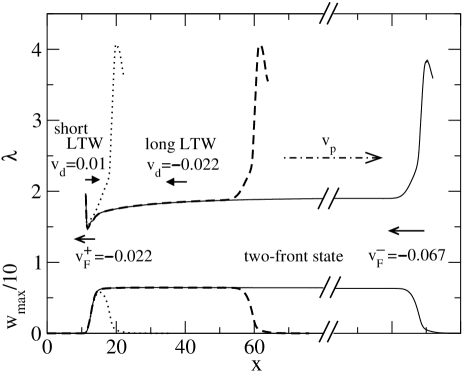
Figure 8: Evolution of the lateral profiles of the wavelength (top) and of the vertical flow amplitude $w_{max}/10$ (bottom) after starting with a very long two-front structure at $r=1.3586,\psi=-0.35$. The $+$front selects in the bulk of the initial two-front structure a saddle-node TW with wavelength $\lambda_{plateau}\sim 1.905$. With $v^{-}_{F}<v^{+}_{F}<0$ the $-$front approaches the $+$front and doing so the velocity of the former goes monotonously towards $v_{F}^{+}$. This transient process ends in a long LTW (dashed line) of constant length $l\simeq 47$ with a plateau wavelength of $1.873$. Its drift and frequency is effectively the same as the respective values of the $+$front which remain unchanged all the time. For comparison the profiles of a short LTW at the same $\psi$ but smaller $r=1.3220$ are shown with dotted lines.

In addition to expanding two-front structures we simulated also shrinking ones for a particular parameter combination ($\psi=-0.35,r=1.3586$, for which $v_{F}^{+}=-0.022>v_{F}^{-}=-0.067$) that is located in Fig. 3(a) at $r<r^{F}_{eq}$. As an example consider the large two-front structure as in Fig. 8. The $+$front selects in the bulk of this initial two-front structure a saddle node TW with wavelength $\lambda_{plateau}\sim 1.905$. In the course of time the velocity $v_{F}^{-}$ of the $-$front approaches that of the $+$front and a stationary LTW forms with length $l\simeq 47$ that drifts with the velocity $v_{d}=v_{F}^{+}=-0.022$ and oscillates with the frequency of the $+$front. These values of the $+$front remain practically unchanged in the whole process.

III Localized traveling wave states

We produced LTW states with very large length $l$ immediately below the Rayleigh number $r^{LTW}_{\infty}=r^{F}_{eq}$. There, $l$ diverges thus marking the upper existence boundary of LTW states. And there, the velocities $v_{F}^{+}$ and $v_{F}^{-}$ of the $+$ and $-$front states, respectively, become equal. See Figs. 2 and 3 for the corresponding results in the range of $-0.4\leq\psi\leq-0.25$ that we have investigated in this paper. Upon decreasing $r$ below the threshold $r^{LTW}_{\infty}(\psi)$ one finds uniquely selected LTW states. Depending on parameters they can coexist stably with front states, extended TW states, and the quiescent basic state.

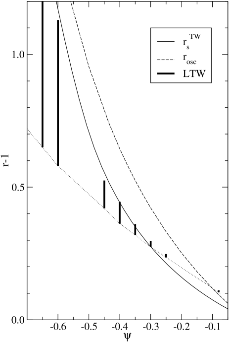
Figure 9: Phase diagram in the $\psi-r$ plane. The vertical bars indicate the range of stable existence of those LTWs that we have numerically simulated. Full and dashed lines refer to the saddle node location $r_{s}^{TW}$ of extended TWs and to their oscillatory Hopf bifurcation threshold $r_{osc}$, respectively; both for a wave number $k=\pi$ . For $\psi\leq-0.25$ the upper existence boundary of LTWs was determined by the requirement that $l$ remained below about 120 in our numerical set-up. The dotted line guides the eye along the lower band limit $r^{LTW}_{min}$ of LTWs. Parameters are $L=0.01,\sigma=10$.

For completeness we include here in Fig. 9 a phase diagram of the $\psi-r$ plane where all the LTWs that we have numerically obtained in the range $-0.65\leq\psi\leq-0.08$ are shown by vertical bars together with the saddle-node location $r_{s}^{TW}(k=\pi)$ of extended TWs (full line) and the oscillatory Hopf bifurcation threshold $r_{osc}(k=\pi)$ for TWs (dashed line). But in this work we focus on the range $-0.4\leq\psi\leq-0.25$.

We should like to emphasize again that we found LTWs for $-0.4\leq\psi\leq-0.25$ only in the parameter regime below $r^{LTW}_{\infty}(\psi)$, i.e., to the left of the crossing points in Figs. 2(a) and 3(a) where the velocities of independent single fronts become equal. Thus, LTWs exist at these $\psi$ only for parameters for which $v_{F}^{+}>v_{F}^{-}$, i.e., for which independent fronts would approach each other: eventually any convective region between them would shrink to zero and the quiescent conductive state would result if this interface motion would continue without change. However, the stabilization effects that allow in such a situation a uniquely selected stable and robust LTW are easily understood with the help of the investigations in the following subsections. On the other hand, for $r>r^{F}_{eq}$ the front velocities are such that a two-front structure expands.

III.1 Transient dynamics towards the selected LTW

A typical transient dynamics towards the uniquely selected LTW is shown in Fig. 6 for $\psi=-0.35$. Here the initial condition was a very broad two-front structure that was prepared at $r=1.3586$ where it shrinks with $v_{F}^{+}>v_{F}^{-}$ [Fig. 3(a)]. In fact, the $-$front moves to the left with a speed that is about three times higher than that of the $+$front.

In the following shrinking process where the $-$front closes up to the $+$front the latter does not change its velocity at all and the former keeps its velocity as long as the bulk TW part between the two fronts is effectively asymptotic, i.e., without lateral variation. This behavior reflects the fact that in such broad two-front structures there is practically no interaction between the fronts when their distance is so large that an asymptotic TW part is realized between the interfaces to conduction. However, the situation changes when the convective region between the interfaces becomes less extended since it requires a finite ’downstream’ growth length behind a $+$interface over which the convection properties still vary with small gradients before the asymptotic TW is reached. The slow lateral variation is best seen in the mixing number $M(x)$ in Fig. 1(e) reflecting the slow variation of the concentration distribution and in the related convective contribution $\langle b\rangle$ [Fig. 1(g)] to the local buoyancy.

When the front separation comes to the order of this length one cannot speak any more of a two-front structure with two independent fronts: For the parameters of Fig. 6 the velocity of the formerly independent $-$front changes continuously from $v_{F}^{-}=-0.067$ to $-0.022$, i.e, to the velocity of the preceeding $+$front and a coherent and robust LTW forms which moves with a drift velocity that is determined by the $+$front, $v_{d}=v_{F}^{+}=-0.022$. During this slowing-down process of the $-$interface its structure changes to that of the characteristic decay interface to conduction of a LTW. Therein the two interfaces, i.e., the former $+$ and $-$fronts, respectively, are in a robust equilibrium with each other at a uniquely selected fixed distance $l$ that depends on $r,\psi$ as shown in Fig. 3(b).

So the $-$interfaces of LTWs and front states do not influence significantly the upstream part of these stuctures. Hence, the local concentration ’barrier’ ahead of the $-$interface does not select the drift velocity of LTWs as speculated previously Barten95II . It is rather the $+$interface that is the more important one.

III.2 Stabilization via front repulsion

Note that it is the ’downstream wake’ in the concentration field of the preceeding $+$front that effectively slows down the $-$front: When the latter reaches the region where the mixing number $M(x)$ [Fig. 1(e)] starts to decrease towards the preceeding $+$front, i.e., when the convective contribution $\langle b\rangle$ [Fig. 1(g)] to the local buoyancy starts to increase then the speed of the approaching $-$interface has to slow down. This distance over which the $+$front influences the $-$front in a two-front structure grows when the Soret coupling becomes stronger. For example at $\psi>-0.3$ a separation of about 160 rolls between the two interfaces is not sufficient to ensure independence.

The sensitive dependence of the velocity of the $-$interface on the concentration-induced buoyancy variation in the ’wake’ behind the $+$front is the main reason for the robust localization mechanism of (long) LTWs. The invasion of conduction into the convective region via the trailing $-$interface is stopped at just that well defined distance from the $+$front where the concentration-induced convective buoyancy $\langle b\rangle$ has become sufficiently large. The latter increases monotonously towards the well mixed region under the $+$interface since this degree of advective mixing decreases gradually in the ’wake’ behind the $+$interface. See, e.g., ref. Jung02 for an explanation of the associated interplay of diffusion and advection which both reduce concentration gradients and the Soret effect which generates them. Of course, the effect of stopping the approaching $-$interface at a particular distance from the $+$interface can be interpreted as an effective repulsive interaction between them.

III.3 Long LTWs

The structural similarity between long LTWs and fronts is documented in Fig. 1. Differences between the full lines (fronts) and the dashed ones (LTW) are visible only in the case of the $-$front in Fig. 1(d,f,h). Here the bulk asymptotic TW that is realized to the left of the $-$front differs slightly from the plateau TW in the LTW.

The above mentioned $\delta C$ redistribution via $<{\bf J}>$ enhances the buoyancy at the $+$interface and leads there to a self-consistent stabilization of convection against invasion of conduction at the $+$front. This mixing effect makes stable LTWs possible even for low heating rates $r$ where neither extended TW convection nor fronts exist.

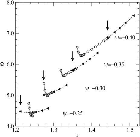
Figure 10: Frequency $\omega$ of $+$fronts (dashed lines with triangles) and of LTWs (full lines with circles) in the respective comoving frame versus $r$ for different $\psi$. Open and shaded circles refer to long and short LTWs, respectively. The frequencies of the former are the same as those of the fronts while short LTWs differ. Arrows indicate the lower limit of existence of the fronts at $r^{F}_{min}=r^{TW}_{s}(k\simeq\pi)$.

Long LTWs are characterized by a wide TW part with a well developed plateau with almost no lateral variation in the convection properties like, e.g., $v_{p}(x)$ or $M(x)$ Jung02 . The TW plateau separates the growth and the decay part of convection at the $+$ and $-$interface, respectively and it provides a communication mechanism favoring one direction: The first region is shielded from the second one by the fast ’downstream’ phase propagation. Like in a single $-$front state the $-$interface of the LTW does not influence the ’upstream’ TW; it only manages the decay transition of the TW vortices into the quiesent fluid. Thus, the $+$front character at the $+$interface is also present in the LTW. And the properties of long LTWs are dominated by and similar to those of the single $+$front at the same $r$ if the latter exists. For example, the drift velocities of long LTWs agree with the values of the corresponding $+$fronts in Figs. 2, 3, 4, 5, 8, 10. Furthermore, they continue to show the same linear variation with $r$ as the $+$fronts even where the latter cease to exist at smaller $r$, cf., the open circles in Fig. 3(a) for the cases of $\psi=-0.35$ and $\psi=-0.4$. Similarly, the variation $\omega(r)$ of long LTWs follows the corresponding one of $+$fronts, cf., open circles and filled triangles in Fig. 10.

A comparison of LTW plateau values with extended TWs and front TWs is presented in Fig. 2(b,c) for $\psi=-0.25$, in Fig. 5 for $\psi=-0.4$, and in Fig. 4 for for all examined $\psi$. At $r^{LTW}_{\infty}=r^{F}_{eq}$ (arrows) there is no difference between the fronts, the diverging LTWs, and the extended saddle TWs.

For decreasing $r$ convection is less stable, the disintegration of the traveling rolls sets in earlier, and the LTW length $l$ is therefore reduced, cf., the inset of Fig. 2 and Fig. 3(b). The smallest plateau wave numbers of LTWs are realized for diverging lengths at $r^{LTW}_{\infty}(\psi)$. With decreasing $r$ one finds a slight increase of $k_{plateau}$ while the wave number selected by a single $+$front remains close to that of the saddle TW.

So this is the LTW bifurcation scenario that we found in the range $-0.4\leq\psi\leq-0.25$ (for a discussion of the scenario at smaller Soret coupling strength cf. Sec. IV.1): Approaching $r^{LTW}_{\infty}$ from below LTWs become indistinguishable from front states when $l\to\infty$. But further below $r^{LTW}_{\infty}$ LTWs differ more and more in particular with respect to the bulk wave numbers as can be seen in Figs. 4 and 5. However, for long enough LTWs with a well developed spatial bulk plateau behavior the frequencies $\omega(r,\psi)$ and drift velocities $v_{d}(r,\psi)$ vary like the corresponding quantities of $+$fronts. This confirms the fact Jung02 that it is the $+$front-like growth interface that selects the properties of a long LTW. Shorter LTWs behave also with respect to the variation of $\omega(r,\psi)$ and $v_{d}(r,\psi)$ somewhat differently.

III.4 Short LTWs

Reducing $r$ one eventually arrives for any $\psi$ at the regime of short LTWs that are marked in Figs 2, 3, and 10 by shaded circles and that are located close to the dotted line in Fig. 9. Here, the dominant influence of the $+$front vanishes eventually in the regime of short LTW pulses. No convection plateau can be identified any more in these structures, cf. the dotted curves in Fig. 6. The prototype of a short LTW consists of a growth interface which is followed directly by the decay of convection so that the whole pulse has to be seen now as one integrated structure that no longer contains front-like independent $+$ and $-$interfaces. Hence, short LTWs show a strong lateral variation of their properties. The shape of their amplitudes superficially resemble the pulse solutions of the complex Ginzburg-Landau equation Niemela90 ; Steinberg91 ; Kolodner91c ; Thual8890 ; Malomed90 ; Hakim90 ; vSaarloos9092 .

Like for long LTWs the stable existence of short pulses below any heating that is necessary to sustain extended TWs is caused by a lateral $\delta C$ redistribution over the pulse. Also its frequency $\omega$ is constant in the frame that comoves with the drift velocity $v_{d}$ of the pulse like for a long LTW. However, compared to long LTWs short LTWs provide a qualitatively new convection structure. They are independent of and cannot even be compared with extended TWs because there is no characteristic wavelength or phase velocity. The special character of short pulses compared with long LTWs or fronts is reflected in the change of the $r$-variation of $v_{d},l,w_{max},\omega$ that can be seen in Figs. 2, 3, and 10 by comparing the dashed circles with the open ones and the filled triangles.

We observed the shortest possible LTWs at the lower end, $r^{LTW}_{min}$, of the $r$ band of LTWs. There they seem to end via a saddle node bifurcation for pulses Hakim90 . These minimal pulses always contained about 5 convection rolls for all Soret couplings $-0.65\leq\psi\leq-0.08$ that we have investigated. This surprising universality of $l_{min}\simeq 5$, i.e., its insensitivity to the values of the actual heating rate $r^{LTW}_{min}$ and the Soret coupling $\psi$ is still unexplained.

Approaching the lower band limit of LTWs their flow intensity steeply drops [Fig. 3(c)] and consequently their frequency increases [Fig. 10] as the degree of advective mixing of the fluid decreases.

III.5 Comparison with LTW models

Several attempts have been made to describe LTWs by simple model equations. Stable pulse solutions of the complex Ginzburg-Landau equation (CGLE) were proposed as a model for confined binary mixture convection Thual8890 . The nonlinear interaction between the local amplitude and frequency seems to be the essential localization mechanism in this approximation. Indeed, one could find localized solutions of increasing length up to the limit of an infinitely long two-front state Malomed90 ; Hakim90 ; vSaarloos9092 . But some basical problems remained: Within the CGLE all pulses drift with the same velocity. This is the critical linear group velocity $v_{g}$ if the coefficients are derived from an asymptotic reduction of the full hydrodynamic field equations. But $v_{g}$ is too fast by a factor of about 20-40 compared with the LTW drift velocity in experiments or simulations Cross88Knobloch88 ; Zimmermann8993 ; Surko87 ; Barten91 ; Luecke92 ; Barten95II ; Jung02 ; Kolodner91a ; Kolodner94 . Brand and Deissler Brand8990 introduced asymmetry in the pulse properties by adding nonlinear gradient terms to the CGLE. A similar extension was given by Bestehorn et al. Bestehorn89 ; Bestehorn888991 within their framework of order parameter equations. Both could produce a very slow drift, even opposite to the phase direction Bestehorn90 . But this kind of nonlinear modification of the linear group velocity involves a balance which seems to be too fragile to explain the occurrence of small pulse velocities over a whole range of $\psi$ and $r$ RieckeL92 .

Another problem was mentioned by van Saarloos and Hohenberg vSaarloos9092 . According to their model of a quintic CGLE nonlinear wide pulses are expected by counting arguments to exist only in a codimension-2 submanifold of the parameter space. Provided there are no hidden symmetries this seems to be incompatible with the robust occurrence of LTWs in experiments. Furthermore, stable pulse solutions seem to exist only in the bistable regime whereas LTWs are known to persist well above the linear onset of extended convection for weakly negative $\psi$ Niemela90 ; Behringer9091 ; Kolodner9091 ; Kolodner91a ; Kolodner91c ; Kolodner91d ; Barten91 ; Barten95II ; Luecke98 . Furthermore, coexisting small stable and wide unstable LTWs were never seen in the CGLE but found in experiments by Kolodner Kolodner94 . Instead, stable broad pulse solutions are found in the model to arise in a saddle node bifurcation together with an unstable branch of smaller ’critical droplets’ near the basic state Hakim90 . Finally, numerical solutions of the field equations show the existence of stable LTWs even below the lowest TW saddle node Jung02 . This makes clear that LTWs are influenced by a localization mechanism that is not contained in the CGLE.

Inspired by simulation results of Barten et al. Barten91 ; Luecke92 which showed the important role of the concentration field for a LTW Riecke RieckeL92 ; RieckeD92 proposed an extension of the Ginzburg-Landau equations. Within a weakly nonlinear expansion he coupled into the standard CGLE as an additional slow variable the amplitude ${\mathcal{C}}$ of an advected mean large-scale concentration mode that influences the growth of the critical modes. A similar idea was advanced already by Glazier et al. Kolodner9091 . The extension can induce an additional amplitude-intability of phase winding solutions to modulated waves. It may be considered as the origin for pulse formation in this ansatz Riecke01 . Riecke showed that the influence of the real ${\mathcal{C}}$-mode alone on the local growth rate (without dispersion) suffices to generate slowly drifting stable pulse solutions even below a supercritical TW-bifurcation RieckeD92 . In this way he modelled a new localization mechanism to explain the robust occurrence of LTWs in binary mixture convection. The amplitude ${\mathcal{C}}$ can be interpreted as a measure for the local mixing state or the mean convection-induced deviation of the vertical concentration gradient from the conductive one. In this way his extended complex Ginzburg-Landau equation (ECGLE) contains in a sketchy way physical effects like the mixing influence on the growth rate and the large-scale concentration redistribution.

Riecke characterized within his model short and long LTWs as dispersion-dominated pulses Riecke96 and states of two fronts that are bounded by the ${\mathcal{C}}$ dynamics RieckeD95 , respectively. He proposed an explanation for their coexistence in stable and unstable form, respectively, by the competition between dispersion-dominated and ${\mathcal{C}}$-dominated localization RieckeD95 ; RieckeL95 .

Note, however, that in contrast to the model used by Riecke our results show stable long LTWs that drift either in or opposite to the direction of phase propagation depending on paramters. It would be interesting to check whether adding a term of the form $v|{\mathcal{A}}|^{2}\partial_{x}{\mathcal{C}}$ to the ${\mathcal{C}}$-equation can stabilize forward drifting long pulses within the model since it models the concentration ’wake’, i.e., the transport of the local mixing state in phase direction by the traveling rolls of amplitude ${\mathcal{A}}$.

Numerical and analytical investigations of the ECGLE predict a hysteretic transition from slow to fast drifting pulses or the existence of oscillatory moving ones Riecke96 . But both were never seen in experiments or simulations. Thus, despite their capability in elucidating some essential mechanisms CGLE type models have the drawback so far that they reproduce only single aspects of LTWs in a qualitative manner. Their range of validity and their predictive power is not well known. And since a satisfactory relation with the full field equations has not been established these models remain somewhat arbitrary.

It appears questionable that weakly nonlinear expansions with spatially slowly varying mode amplitudes are approriate at all in view of the very large Péclet numbers, $\cal O$(1000), measuring the strength of the nonlinearity in the concentration balance. Thus, so far numerical simulations of the full field equations seem to be the appropriate tool besides careful experiments to gather insight into the specific physical mechanisms for LTW formation in binary mixture convection.

IV Comparison with experiments and discussion

IV.1 Small Soret coupling strength

An inspection of Figs. 2, 3, and 9 shows that the lower band limit $r^{LTW}_{min}$ for the existence of short LTWs and the crossing value, $r^{F}_{eq}=r^{LTW}_{\infty}$, where the velocities of free fronts become equal approach each other when $|\psi|$ decreases. Thus, one can foresee an interval of moderately negative $\psi$ where short and long LTWs can be found close to $r^{LTW}_{\infty}$. In this case the upper band limit for the existence of stable LTWs should be defined by a backward saddle-node bifurcation at $r_{s}^{LTW}$ where the branches of stable short and unstable long LTWs annihilate each other.

Hence, we expect that the upper parts of the bifurcation diagrams of $l$ versus $r$ in the inset of Figs. 2 and in Fig. 3(b) curve backwards towards smaller $r$ when $|\psi|$ decreases further below the values of the two figures. In this way the shape of the curve $l(r)$ would change continuously from the form shown in Fig. 11(b) to the one in Fig. 11(a). The former shows schematically the bifurcation behavior of $l(r)$ that we have determined numerically for $\psi\lesssim-0.25$. In fact, at $\psi$ slightly larger than -0.25 we expect the appearence of the saddle-node in the curves $l(r)$. Fig. 11(a) is a schematic representation of experimental results of Kolodner Kolodner94 for $\psi=-0.127$ as presented in his Fig. 5. He stabilized by an adaptive heating mechanism long unstable LTWs in coexistence with short stable ones. Thus, the unstable LTW solution branch [dashed line in Fig. 11(a)] forms for $r^{LTW}_{\infty}\leq r\leq r_{s}^{LTW}$ a separatrix between the domains of attraction of expanding two-front structures to the right of the dashed line in Fig. 11(a) and the domain to the left of the dashed line leading to stable narrow pulses or the basic state. Furthermore, small LTWs that are prepared at $r<r_{s}^{LTW}$ will evolve into expanding two-front structures when $r$ is increased above $r_{s}^{LTW}$.

Note that in Kolodner’s experiment Kolodner94 done at $\psi=-0.127$ the upper band limit $r_{s}^{LTW}$ of LTWs lies above the Hopf bifurcation threshold $r_{osc}$ for extended TWs where perturbations of the quiescent fluid can grow. Therefore, one has to address there questions related to linear and nonlinear convective versus absolute instability Chomaz92 ; Bu99 , to linearly selected so-called pulled fronts versus nonlinearly selected so-called pushed fronts vSaarloos9092 ; vSaarloos03 , and to the robustness and stability of nonlinear fronts under emission or absorption of TW perturbations that can grow in the region occupied by the quiescent fluid.

IV.2 Strong Soret coupling strength

For stronger negative $\psi$ the measured LTW properties agree qualitatively well with our results. For example, the ’arbitrary-width confined states’ found in experiments Kolodner93II for $\psi=-0.253$ at a single Rayleigh number are to be identified as two-front structures. A quantitative comparison is difficult due to the difference in the boundary conditions: We simulated two-dimensional convection assuming translational symmetry in $y$-direction while the narrow experimental convection channels impose no-slip conditions at the walls perpendicular to the roll axes. There are three effects that account for the difference beteen experiments and simulations.

First, the characteristic Rayleigh numbers in the experiments are higher. This is already known from the suppression of oscillatory or steady convection instabilities in narrow channels Platten84 ; CJT97 ; AlBa04 . The no-slip conditions at the side-walls generate a nontrivial $y$-variation of the velocity field that introduces additional internal friction and that has to be compensated by a higher heating rate Catton72 ; Ohlsen90 ; Bensimon90 .

Second, the LTW drift velocities in the experiment have the global tendency to lie below those of the simulations. For example, for $\psi=-0.253$ the experimental LTWs Kolodner93II ; Kolodner94 move opposite to the phase velocity whereas according to our calculations $v_{d}$ should be around $0.05$. Again, we attribute this difference to the fact that we neglect gradients in $y$-direction. They change the concentration redistribution dynamics in particular at the $+$interface of the LTW which determines the drift velocity. In this context one has to note that already weak inhomogeneities in a convection cell can slow down and even pin the LTW movement Kolodner91a ; Kolodner91c ; Kolodner93II . Finally, the influence of the different boundaries on the frequencies, phase velocities, and wave numbers of confined states are totally unknown.

Also when comparing quantitatively our results for fronts with experiments one should take into account the above discussed points.

Extrapolating our results for the front velocities to more negative $\psi$ beyond $\psi=-0.4$ we see that already at the lowest TW saddle location $r_{min}^{TW}$ two-front stuctures would expand with $v_{F}^{-}>v_{F}^{+}$. In other words, the velocity crossing point $r^{F}_{eq}$ is no longer above $r_{min}^{TW}$ but has virtually moved below the lowest TW saddle location where in fact no fronts exist. On the other hand, LTWs still exist in this $r$-range with length increasing with $r$. However, $l(r)$ does not seem to diverge anymore as for $-0.4\lesssim\psi$ which is compatible with the absence of fronts moving with the same velocity.

IV.3 Wall-attached confined structures

Laterally confined convection patches of traveling rolls were found in the early experiments Moses87Heinrichs87 ; Fineberg88Steinberg89 ; Niemela90 ; Kolodner91b that were done in narrow rectangular convection channels in the form of so-called wall-attached confined structures (WACS). They were localized near one of the short end walls closing the channel.

These WACS can be understood with our knowledge of fronts and free LTWs. For example, for the weakly negative $\psi$ used in the early experiments the phase velocity of the WACS was directed towards the wall to which they were attached. Indeed, for such parameters mainly short LTWs occur with drift velocities in phase direction so that they would end as WACS of the above described type in finite length channels. Furthermore, the measured WACS profiles of phase velocity $v_{p}(x)$, of wavelength $\lambda(x)$, and their decrease of frequency with increasing $r$ Fineberg88Steinberg89 ; Steinberg91 ; Kolodner91b agree qualitatively with the typical behavior of free short LTWs.

The connection between WACS and free LTWs was more explicitly demonstrated by Kolodner Kolodner90 for more negative separation ratios $\psi=-0.24$ and $-0.408$: He prepared a free LTW pulse with large phase velocity (a ’fast confined state’ in his terminology) which drifted slowly opposite to the direction of phase propagation towards an end wall of the convection channel and became there a WACS (a ’slow confined state’ in his terminology) with lower phase velocity being directed away from the wall. In this WACS the phase generating ’trailing front’, i.e., the analogue of the $+$interface is pinned at the wall and therefore without solutal gradients to the quiescent fluid as in a free LTW. The absence of these concentration variations at the $+$interface implies and allows a lateral concentration redistribution over the whole state at lower levels of the mixing number $M$ in WACS as compared to free LTWs. Consequently, the phase velocities and frequencies of WACS are smaller than those of the respective free LTWs. A less dramatic drop of frequency was observed also between forward drifting LTWs and short WACS at $\psi=-0.047$ Steinberg91 .

Due to their better mixing capability, i.e., smaller $M$ it is very probable that short WACS can exist for heating rates below the lower band limit $r^{LTW}_{min}$ of stable LTW pulses — at least in the case where the phase velocity is directed away from the wall. It would be very interesting to test this conjecture experimentally, in particular for strongly negative $\psi$. There $r^{LTW}_{min}$ itself lies already well below the range of stable TWs Jung02 and so the WACS would lie even lower. An inportant hint that this conjecture is right is given by Ning et al. Ning96 . They have performed two-dimensional simulations of a finite-length convection channel with realistic boundary conditions for $\psi=-0.47,\sigma=13.8$, and $L=0.01$. Neglecting the slight difference in $\sigma$ their results should be comparable with our work. They found short WACS at $r=1.35$ which is according to our results far below the TW saddle nodes for this separation ratio and also below the lower band limit $r^{LTW}_{min}$ of free LTWs for $\psi=-0.40$. However, these authors claim — we think, incorrectly — that their WACS lie above the saddle-node location $r_{s}^{TW}$ of extended TWs.

IV.4 LTW and front stability

In the previous section we have shown that the $+$interface where the convection rolls grow in ’downstream’ direction out of the quiescent fluid plays the dominant role for the stability of LTWs. While the $-$interface where the decaying rolls are advected into the quiescent fluid does not play a decisive role. This is clearly confirmed in pulse collision experiments Kolodner9091 .

Fast TW pulses — linear ones with small amplitude as well as nonlinear ones with larger amplitude — were completely absorbed by a LTW when the pulses hit the $-$interface of the LTW, i.e., when the pulse velocity is directed opposite to and towards the phase velocity of the LTW. Then the collision with the pulse affects only the $-$interface itself and perturbations are quickly advected out of the LTW and do not propagate upstream towards the $+$interface. For the same reason double-LTW states of two counter propagating waves can persist over a long time Kolodner9091 or even be stable Kolodner91d . Moreover, a pair of LTWs that have their phase propagation directed towards each other and that interact with each other via their decay interfaces is seen to be stable over a substantially wider $r$-range than two LTW pulses which are connected at their growth interfaces Kolodner91d . Obviously the latter case is more critical for the structural integrity of the involved LTWs.

A LTW is most likely destroyed when another wave with the same direction of phase propagation infiltrates its phaseflow at the growth region. Then, while growing the perturbations can be transmitted into the strongly nonlinear bulk part of the LTW and can destroy its coherence.

The different selection and stability properties of the $+$ and $-$interfaces were already observed in transient convection behavior in various experiments (see for example Kolodner88 ; Bensimon90 ), however without further investigation.

IV.5 Defected confined states

The fact that ($i$) different $-$fronts with different bulk TW parts are possible as stable coexisting states and that ($ii$) a $+$front interface is in general stable against downflow perturbations opens the possibility for another kind of stable long confined TWs: Therein rolls with low wavelength grow out of the quiescent fluid in a ’normal’ growth part. In the bulk an incoherent phase front connects this fast wave that is coming from the $+$interface with a slow wave of higher wavelength and larger amplitude via spatiotemporal dislocations as, e.g., in Fig. 7. The transition could take place via one or more intermediate convection states. Eventually this slow TW convection undergoes a decay transition into the basic state via a coherent $-$interface. Such ’defected confined states’ are indeed observed in annular containers Bensimon90 ; Behringer9091 and were studied by Kolodner Kolodner94 . He found such structures only for $\psi\leq-0.21$. One may speculate that for these separation ratios the bulk TW that is selected by and behind the $+$interface is absolutely unstable against the slow wave in the further ’downstream’ part. This could explain the existence of persistent roll pair annihilations without the need of fluctuations.

We finally mention that the occurrence of phase annihilating dislocations between a growth part and the downstream convection was observed for moderately negative $\psi$ already in narrow rectangular containers Kolodner91b . Furthermore, end-wall induced Eckhaus instabilities of downstream TW states have been seen in simulations BuLu99 .

V Conclusion

For parameters where the conductive quiescent fluid is stable and where spatially extended TW solutions bifurcate subcritically out of it we have investigated in quantitative detail relaxed, strongly nonlinear oscillatory convection structures with one or two interfaces to the quiescent fluid, i.e, fronts and LTWs, respectively. They are time-periodic global nonlinear modes: in the frame that is comoving with the respective front velocity $v_{F}$ or with the LTW drift velocity $v_{d}$ the oscillations have everywhere the same period.

Fronts come in two varieties. In a $+$front state the quiescent fluid is located ’upstream’, i.e., phase propagates out of it into convection. In a $-$front the quiescent fluid is located in ’downstream’ direction and phase moves out of convection into conduction.

The lowest Rayleigh number for the existence of fronts is the lowest saddle-node location of extended TWs, $r^{F}_{min}=r^{TW}_{min}$: below it there are no TWs to which the interface from conduction can connect. However, LTWs of finite length $l$ can coexist bistably together with the conductive state well below the lowest TW saddle when the Soret coupling is sufficiently negative, $r^{LTW}_{min}<r^{TW}_{min}$. Furthermore, we have arguments that WACS at end walls of rectangular channels can exist even at smaller $r$ than LTWs.

Central for understanding fronts and LTWs is a large-scale concentration redistribution that influences the buoyancy at the interfaces to conduction in different ways than in the bulk TW parts. For example, at the $+$interfaces of fronts and LTWs alike there is a buoyancy overshoot which is sufficiently large to sustain local convection growth there and that can cause even invasion of convection into the stable quiescent fluid. At the $-$interface the lateral buoyancy variation is such as to induce the decay of the approaching convection rolls into the conductive state.

Front velocities as well as LTW drift velocities are much smaller than the phase velocities of the carrier waves for reasons that are related to the concentration redistribution dynamics. The velocities of $+$fronts decrease with growing $r$ while those of $-$fronts increase. At some $r^{F}_{eq}$ they become equal so that both fronts move with the same velocity. At this Rayleigh number the length $l$ of the LTWs diverges and there, and strictly speaking only there, the limiting LTW can be seen as a state consisting of two fronts. However, $+$fronts and long LTWs have almost identical propagation velocities and frequencies. Furthermore, they select a similar bulk wave number. The selected frequencies and bulk wave numbers are close to those of a saddle-node TW. In fact, it is the $+$front-like growth interface that selects the properties of long LTWs.

Small amplitude extended TW perturbations of the conductive state oscillate with the large Hopf frequency. But the global-mode oscillation is restrained by the requirement that its frequency has to allow stable developed bulk TW convection. It is interesting to note that the $+$interface connecting conduction with convection selects the largest possible frequency eigenvalue that meets this requirement, namely the TW saddle-node frequency. All our $+$fronts select bulk TW wave numbers close to the large-$k$ branch of the TW saddle-node curve, i.e., wave numbers that are too large to be Eckhaus stable. However, these TWs are only convectively unstable: perturbations can grow but while doing so they are advected sufficiently fast downstream in the direction of the TW phase propagation so that they cannot influence the upstream part of the $+$front state in a persistent way.

While $+$front states seem to be uniquely selected we could produce for a fixed $r$ different coherent $-$fronts that were characterized in the bulk part by different wave numbers and frequencies close to the TW saddles. The decay interface adjusts itself to the respective bulk TW part but does not exert an influence in ’upstream’ direction on the bulk convection within a coherent $-$front. In contrast, the growth under a $+$interface induces in downstream direction a long concentration ’wake’ that is characteristic for $+$fronts and long LTWs and of special importance for the latter.

Here it is interesting to notice that all the interfaces of fronts and LTWs consist typically only of about 3-4 convection rolls. We furthermore should like to mention that $+$interfaces of fronts and LTWs always locate a minimal wavelength. Its value, $\lambda_{min}\sim 1.4$, is remarkably universal for all $r$ and $\psi$ that we have simulated. This is unexplained so far.

We have also prepared initial two-front stuctures by connecting a $+$front and a $-$front with a common long bulk TW. When $r>r^{F}_{eq}$ they expand. But at $r<r^{F}_{eq}$ they shrink towards a uniquely selected LTW of fixed length $l$. Here the ’downstream wake’ in the concentration field of the preceeding $+$front exerts an effective repulsion on the approaching $-$interface: the invasion of conduction via the latter is stopped at a well defined distance $l$ that is determined by the concentration-induced buoyancy levels in the ’wake’ of the $+$front.

LTWs shortly below $r^{F}_{eq}$ (where LTW with diverging $l$ are possible) are very long. Their drift velocities, frequencies, and many stuctural properties are similar to those of $+$fronts. Decreasing $r$ the LTW length decreases and one eventually arrives for any $\psi$ at the regime of short LTWs that lies for strongly negative $\psi$ well below the TW saddle-nodes. These short LTWs without a convection plateau are qualitatively different structures. This is also reflected by their drift velocities and frequencies showing a variation with $r$ that differs from those of long LTWs. The shortest possible LTWs are realized at the lower end of the $r$ band of LTWs. These minimal pulses always contained about 5 convection rolls for all Soret couplings that we have investigated. This surprising universality of $l_{min}\simeq 5$ remains to be explained.

Figure 1: Typical structures of a coherent $+$front (left) and of a $-$front (right) with nearly the same asymptotic wavelength $\lambda=1.90$. Only the vicinity of the respective interfaces between convection and conduction is shown. Both fronts propagate to the left ($v^{+}_{F}=-0.022,v_{F}^{-}=-0.067$), i.e., opposite to the direction of the phase velocity $v_{p}$. (a, b) Color coded snapshot of concentration deviation $\delta C$ from its global mean in a vertical cross section of the layer. The color code is shown at the right end of (b). (c, d) Instantaneous lateral wave profile at midheight, $z=0$, of $\delta C$ (green), vertical velocity $w$ (blue), and its envelope. Arrows mark the positions where $w$ has grown up to $v_{p}$. (e, f) Mixing number $M$ (green), Eq. (3), and phase velocity $v_{p}$ (black) of the nodes of $w$ in the comoving frames. The variation of $\lambda(x)=2\pi v_{p}(x)/\omega$ is the same since the frequency $\omega$ is a global constant. (g, h) Time averaged deviations from the conductive state at $z=-0.25$ for concentration (green), temperature (red), and their sum ($<b>$) measuring the convective contribution to the buoyancy. (i, j) Streamlines of the averaged concentration current $<{\bf J}>$ (green) and velocity field $<{\bf u}>$ (blue). The latter results from $<b>$ and documents roll shaped contributions of $<{\bf u}><\delta C>$ to $<{\bf J}>$ at the interfaces. Thick blue and green arrows indicate $<{\bf u}>$ and transport of positive $\delta C$ (alcohol surplus), respectively. Temporal averaging is always performed in the frame comoving with the respective front velocity. Dashed lines show the decay part of the long LTW that coexists at the same parameters ($r=1.3586,\psi=-0.35,L=0.01$) with the fronts. Differences between the interfaces of the $+$front and the corresponding LTW interface are not visible on the scale of the above plots.

Figure 6: Typical spatio-temporal evolution of a $+$front. Shown are the extrema positions of the vertical velocity field $w$. The initial condition at time $t=-5$ (not visible) consisted of an extended TW for $x>8$ with wavelength $\lambda=1.85$ and phase velocity $v_{p}=1.032$ and quiescent fluid for $x<8$. Boundary conditions are conduction at $x=0$ and $f(x=160)=f(x=160-1.85)$ that imposes at $x=160$ a wavelength of $\lambda=1.85$. First, a pulse that causes a quite regular sequence of roll-pair annihilation events (lower line of defects) propagates to the right with velocity greater than $v_{p}$. The intermediate wave pattern resulting from this primary sequence of defects is then transformed via further, somewhat erratically occurring phase defects into the fast asymptotic TW with $\lambda=1.80,v_{p}=1.258$ that is favoured by the $+$front. The boundary condition at $x=160$ that imposes a ’wrong’ wavelength there does not influence the bulk behavior which is selected by the front. Parameters are $r=1.237,\psi=-0.25$.

Figure 7: Spatio-temporal dynamics of a front-selected TW pattern that is convectively Eckhaus unstable. Shown are the extrema positions of the vertical velocity field $w$. The front selects a bulk TW with wavelength $\lambda\sim 1.72$ that is strongly Eckhaus unstable: While beeing advected ’downstream’ phase deformations (that are caused, e.g., by computer ’noise’) grow sufficiently fast to reach a critical amplitude within the system length. Then two neighboring rolls are annihilated. That increases the wavelength and decreases the phase velocity towards Eckhaus stable values. Parameters are $r=1.26,\psi=-0.25$.

Figure 11: Schematic bifurcation diagrams of LTW length $l$ versus $r$. (a) experimental results Kolodner94 obtained for $\psi=-0.127$ with dashed line denoting unstable states (cf., text for further explanation); (b) numerically obtained bifurcation behavior for $-0.4\leq\psi\leq-0.25$.

References

- (1) M. C. Cross and P. C. Hohenberg, Rev. Mod. Phys. 65, 851 (1993).
- (2) For 5 weight percent of ethanol mixed into water at the separation ratio measuring the Soret coupling strength CH93 is ; see P. Kolodner, H. L. Williams, and C. Moe, J. Chem. Phys. 88, 6512 (1988).
- (3) R. W. Walden, P. Kolodner, A. Passner, and C. M. Surko, Phys. Rev. Lett. 55, 496 (1985).
- (4) E. Moses, J. Fineberg, and V. Steinberg, Phys. Rev. A 35, R2757 (1987); R. Heinrichs, G. Ahlers, D. S. Cannell, ibid. 35, R2761 (1987).
- (5) K. E. Anderson and R. P. Behringer, Phys. Lett. A 145, 323 (1990); K. E. Anderson and R. P. Behringer, Physica D 51, 444 (1991).
- (6) B. I. Winkler and P. Kolodner, J. Fluid Mech. 240, 31 (1992).
- (7) P. Kolodner, Phys. Rev. E 50, 2731 (1994).
- (8) H. Touiri, J. K. Platten, and G. Chavepeyer, Eur. J. Mech. B 15, 241 (1996).
- (9) E. Kaplan, E. Kuznetsov, and V. Steinberg, Phys. Rev. E 50, 3712 (1994).
- (10) C. M. Surko, D. R. Ohlsen, S. Y. Yamamoto, and P. Kolodner, Phys. Rev. A 43, R7101 (1991).
- (11) C. M. Aegerter and C. M. Surko, Phys. Rev. E 63, 46301 (2001).
- (12) L. Ning, Y. Harada, and H. Yahata, Prog. Theor. Phys. 98, 551 (1997).
- (13) O. Batiste, E. Knobloch, I. Mercader, and M. Net, Phys. Rev. E 65, 016303 (2001).
- (14) D. Jung and M. Lücke, Phys. Rev. Lett. 89, 054502 (2002).
- (15) C. Fütterer and M. Lücke, Phys. Rev. E 65, 036315 (2002).
- (16) D. Jung, P. Matura, and M. Lücke, Eur. Phys. J. E. 15, 293 (2004).
- (17) P. Matura, D. Jung, and M. Lücke, Phys. Rev. Lett. 92, 254501 (2004).
- (18) D. Bensimon, P. Kolodner, C. M. Surko, H. Williams, and V. Croquette, J. Fluid Mech. 217, 441 (1990).
- (19) P. Kolodner, Phys. Rev. A 46, 6452 (1992).
- (20) P. Büchel, Ph.D. thesis, Universität des Saarlandes, 1999.
- (21) C. M. Surko and P. Kolodner, Phys. Rev. Lett. 58, 2055 (1987).
- (22) A. Alonso and O. Batiste, Theoret. Comput. Fluid Dynamics 18, 239 (2004).
- (23) P. Kolodner, J. A. Glazier, and H. Williams, Phys. Rev. Lett. 65, 1579 (1990); J. A. Glazier, P. Kolodner, and H. Williams, J. Stat. Phys. 64, 945 (1991).
- (24) M. Lücke, W. Barten, P. Büchel, C. Fütterer, St. Hollinger, and Ch. Jung, in Evolution of Structures in Dissipative Continuous Systems, edited by F. H. Busse and S. C. Müller, (Springer, Berlin, 1998), p. 127.
- (25) W. Barten, M. Lücke, M. Kamps, and R. Schmitz, Phys. Rev. E 51, 5636 (1995).
- (26) W. Barten, M. Lücke, M. Kamps, and R. Schmitz, Phys. Rev. E 51, 5662 (1995).
- (27) P. Kolodner, D. Bensimon, and C. M. Surko, Phys. Rev. Lett. 60, 1723 (1988).
- (28) P. Kolodner, Phys. Rev. Lett. 66, 1165 (1991)
- (29) V. Steinberg and E. Kaplan, in Spontaneous Formation of Space-Time Structures and Criticallit, edited by T. Riste and D. Sherrington (Kluwer, Boston, 1991), p. 207.
- (30) J. J. Niemela, G. Ahlers, and D. S. Cannell, Phys. Rev. Lett. 64, 1365 (1990).
- (31) P. Kolodner and J. A. Glazier, Phys. Rev. A 42, R7504 (1990); J. A. Glazier and P. Kolodner, ibid. 43, 4269 (1991).
- (32) P. Kolodner, Phys. Rev. A 44, 6448 (1991).
- (33) P. Kolodner, Phys. Rev. A 44, 6466 (1991).
- (34) P. Kolodner, Phys. Rev. E 48, R4187 (1993).
- (35) W. Barten, M. Lücke, and M. Kamps, Phys. Rev. Lett. 66, 2621 (1991).
- (36) M. C. Cross, Phys. Rev. Lett. 57, 2935 (1986); Phys. Rev. A 38, 3593 (1988); Physica D 37, 315 (1989).
- (37) H. R. Brand, P. S. Lomdahl, and A. C. Newell, Phys. Lett. A 118, 67 (1986); Physica D 23, 345 (1986).
- (38) J. Fineberg, V. Steinberg, and P. Kolodner, Phys. Rev. A 41, R5743 (1990).
- (39) P. Kolodner and C. M. Surko, Phys. Rev. Lett. 61, 842 (1988); P. Kolodner, C. M. Surko, and H. L. Williams, Physica D 37, 319 (1989).
- (40) J. Fineberg, E. Moses, and V. Steinberg, Phys. Rev. Lett. 61, 838 (1988); Phys. Rev. A 38, R4939 (1988); V. Steinberg, J. Fineberg, E. Moses, and I. Rehberg, Physica D 37, 359 (1989).
- (41) M. Bestehorn, R. Friedrich, and H. Haken, Z. Phys. B 77, 151 (1989).
- (42) P. Kolodner, Phys. Rev. E 47, 1038 (1993).
- (43) P. Kolodner, A. Passner, C. M. Surko, and R. W. Walden, Phys. Rev. Lett. 56, 2621 (1986).
- (44) P. Kolodner, C. M. Surko, A. Passner, and H. L. Williams, Phys. Rev. A 36, R2499 (1987).
- (45) E. Moses and V. Steinberg, Phys. Rev. A 34, R693 (1986).
- (46) P. Kolodner, Phys. Rev. A 42, R2475 (1990).
- (47) P. Kolodner, Phys. Rev. A 43, 2827 (1991).
- (48) H. Yahata, Prog. Theor. Phys. 85, 933 (1991).
- (49) L. Ning, Y. Harada, and H. Yahata, Prog. Theor. Phys. 96, 669 (1996).
- (50) L. Ning, Y. Harada, and H. Yahata, Prog. Theor. Phys. 97, 831 (1997).
- (51) L. D. Landau and E. M. Lifschitz, Course of Theoretical Physics, (Pergamon Press, Oxford, 1993), Vol. 6.
- (52) J. K. Platten and J. C. Legros, Convection in Liquids, (Springer, Berlin, 1984).
- (53) W. Hort, S. J. Linz, and M. Lücke, Phys. Rev. A 45, 3737 (1992).
- (54) St. Hollinger and M. Lücke, Phys. Rev. E 52, 642 (1995).
- (55) J. L. Liu and G. Ahlers, Phys. Rev. Lett. 77, 3126 (1996).
- (56) G. W. T. Lee, P. Lucas, and A. Tyler, J. Fluid Mech. 135, 235 (1983).
- (57) F. H. Harlow and J. E. Welch, Phys. Fluids 8, 2183 (1965); J. E. Welch, F. H. Harlow, J. P. Shannon, and B. J. Daly, Los Alamos Scientific Laboratory of the University of California, Report No. LA-3425, 1966 (unpublished); C. W. Hirt, B. D. Nichols, and N. C. Romero, ibid. Report No. LA-5852, 1975 (unpublished).
- (58) R. Peyret and T. D. Taylor, Computational Methods in Fluid Flow (Springer, Berlin, 1983).
- (59) W. van Saarloos and P. C. Hohenberg, Phys. Rev. Lett. 64, 749 (1990); Physica D 56, 303 (1992).
- (60) W. van Saarloos, Phys. Rep. 386, 29 (2003); and references therein.
- (61) M. van Hecke, W. van Saarloos, and P. C. Hohenberg, Phys. Rev. Lett. 71, 2162 (1993).
- (62) P. Colet, D. Walgraef, and M. San Miguel, Eur. Phys. J. B 11, 517 (1999).
- (63) A. Couairon and J. M. Chomaz, Physica (Amsterdam) 158D, 129 (2001).
- (64) A. Szprynger and M. Lücke, Phys. Rev. E 67, 046301 (2003).
- (65) L. Meignin, P. Gondret, C. Ruyer-Quil, and M. Rabaud, Phys. Rev. Lett. 90, 234502 (2003).
- (66) P. Büchel and M. Lücke, Phys. Rev. E 63, 016307 (2000).
- (67) St. Hollinger, P. Büchel, and M. Lücke, Phys. Rev. Lett. 78, 235 (1997).
- (68) S. J. Linz, M. Lücke, H. W. Müller, and J. Niederländer, Phys. Rev. A38, 5727 (1988).
- (69) W. Barten, M. Lücke, W. Hort, and M. Kamps, Phys. Rev. Lett. 63, 376 (1989).
- (70) G. W. Baxter, K. D. Eaton, and C. M. Surko, Phys. Rev. A 46, R1735 (1992).
- (71) P. Kolodner, Phys. Rev. A 46, R1739 (1992); ibid. 46, 6431 (1992).
- (72) I. Mercader, A. Alonso, and O. Batiste, Eur. Phys. J. E. 15, 311 (2004).
- (73) O. Thual and S. Fauve, J. Phys. France 49, 1829 (1988); S. Fauve and O. Thual, Phys. Rev. Lett. 64, 282 (1990).
- (74) V. Hakim, P. Jakobsen, and Y. Pomeau, Europhys. Lett. 11, 19 (1990).
- (75) B. A. Malomed and A. A. Nepomnyashchy, Phys. Rev. A 42, 6009 (1990).
- (76) M. Lücke, W. Barten, and M. Kamps, Physica D 61, 183 (1992).
- (77) M. C. Cross and K. Kim, Phys. Rev. A 37, 3909 (1988); E. Knobloch and D. R. Moore, ibid. 37, 860 (1988).
- (78) W. Schöpf and W. Zimmermann, Europhys. Lett. 8, 41 (1989); Phys. Rev. E 47, 1739 (1993).
- (79) H. R. Brand and R. J. Deissler, Phys. Rev. Lett. 63, 2801 (1989); R. J. Deissler and H. R. Brand, Phys. Lett. A 146, 252 (1990).
- (80) M. Bestehorn, R. Friedrich, and H. Haken, Z. Phys. B 72, 265 (1988); 75, 265 (1989); Physica D 37, 295 (1989); M. Bestehorn, Europhys. Lett. 15, 473 (1991).
- (81) M. Bestehorn and H. Haken, Phys. Rev. A 42, 7195 (1990).
- (82) H. Riecke, Phys. Rev. Lett. 68, 301 (1992).
- (83) H. Riecke, Physica D 61, 253 (1992).
- (84) A. Roxin and H. Riecke, Physica D 156, 19 (2001).
- (85) H. Riecke, Physica D 92, 69 (1996).
- (86) H. Herrero and H. Riecke, Physica D 85, 79 (1995).
- (87) H. Riecke and W. J. Rappel, Phys. Rev. Lett. 75, 4035 (1995).
- (88) J. M. Chomaz, Phys. Rev. Lett. 69, 1931 (1992).
- (89) Ch. Jung, Numerische Simulationen dreidimensionaler Konvektionsstrukturen in binären Fluiden mit positiver Soretkopplung, Ph.D. thesis, Universität des Saarlandes, 1997.
- (90) I. Catton, J. Heat Mass Transfer 15, 665 (1972).
- (91) D. R. Ohlsen, S. Y. Yamamoto, C. M. Surko, and P. Kolodner, Phys. Rev. Lett. 65, 1431 (1990).
- (92) P. Büchel and M. Lücke, Entropie 218, 22 (1999).