Singularities of Hele-Shaw Flow and Shock Waves in Dispersive Media

Abstract

We show that singularities developed in the Hele-Shaw problem have a structure identical to shock waves in dissipativeless dispersive media. We propose an experimental set-up where the cell is permeable to a non-viscous fluid and study continuation of the flow through singularities. We show that a singular flow in this, non-traditional cell is described by the Whitham equations identical to Gurevich-Pitaevski solution for a regularization of shock waves in Korteveg-de-Vriez equation. This solution describes regularization of singularities through creation of disconnected bubbles.

1. Introduction. A broad class of non-equilibrium growth processes in two dimensions are characterized by a common law: the velocity of the growing interface is determined by the gradient of a harmonic field (often referred to as Laplacian growth) review .

Growth processes determined by a harmonic field, where no cut-off scale is introduced, are important. The theory of this kind of growth is deeply related to fundamental aspects of conformal maps, integrable systems, 2D quantum gravity and random matrices ourpapers . However, singularities makes this problem ill-defined and thus not achieved experimentally.

The goal of this Letter is two-fold. One is to suggest an experimentally achievable set-up, where a high-rate flow can continue through singularities, without being curbed by dissipative forces. Another is to stress a deep and important parallel between the singularities of growing interface and “gradient catastrophes” known in the theory of shock waves in dispersive media. The Korteveg-de-Vriez (KdV) and other nonlinear waves equations feature this phenomenon. This relation allows one to effectively study complicated singular processes.

The relation between the Hele-Shaw problem and dispersive nonlinear waves suggests a unique regularization, namely one which plays a similar role as dispersion of nonlinear waves. There, dispersion, (no matter how small it is) becomes crucial near a singularity, converting shock waves to oscillatory structures singular .

2. The Hele-Shaw flow. The Hele-Shaw cell is a narrow space between two plates filled by incompressible viscous liquid (say oil). Air (regarded as inviscid and incompressible) occupies a part of the cell forming one or several bubbles. Traditionally air is pumped into one bubble, while oil is extracted from the cell at a constant rate $Q>0$ through the edges placed at infinity. Without surface tension, the interface may develop singular cusps at a finite time review . At this moment the problem becomes ill-posed.

We suggest a novel set up where the upper plate is permeable to air and is connected to a reservoir of air. Neither plates are permeable to oil. This set-up may be achieved by sticking a Gortex-like material to glass plates having small perforations (Fig.1). We thus assume that all air bubbles are kept at the same atmospheric pressure. We also consider a retraction problem, where oil is extracted from the cell, i.e. $Q<0$.

In both cells the flow obeys the same local equations (D’Arcy’s law): The local velocity of oil, averaged over the gap between the plates, is proportional to a gradient of pressure $p$. In an incompressible fluid pressure is a harmonic function. Thus the normal velocity of the interface, $v_{n}$, is proportional to the normal derivative of pressure, and in proper units $v_{n}=-\,\partial_{n}p$. If in addition surface tension is ignored, the pressure is continuous across the interface, and may be set to $p=0$ within each bubble. Thus the pressure solves the exterior Dirichlet boundary value problem: $\Delta p=0$, with $p=0$ on the boundary, and $p\to-Q\log|z|$ at infinity.

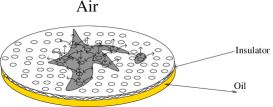
Figure 1: Schematic Hele-Shaw experimental set up. Shaded region represents a small bubble of air in the ambient oil. The insulator is permeable to air but not to oil.

3. Bubble break-off and merging. Let us now describe an air retraction process in our experimental set up. A typical local evolution of an air bubble consists of few phases illustrated in Fig. 2: (i) As oil is injected, the air bubble contracts; (ii) The air bubble forms a singular narrow neck and breaks-up into one or several disconnected bubbles; (iii) All bubbles subsequentially contract, while loosing air through the upper plate.

As we show in this Letter, the method of regularization of shock waves provides a detailed description of retraction evolution in the limit of zero surface tension. This is in contrast with the injection process in a traditional Hele-Shaw cell where solutions at the zero surface tension limit are valid only until a cusp is formed. This difference, suggests that surface tension is a non-singular perturbation in our new experimental setup.

4. Dispersive regularization of shock waves. The term shock wave is usually used to describe nonlinear waves in presence of dissipation. In the absence of dissipation the shock-wave behavior is different. It is resolved by converting to oscillations. The method to study this complicated behavior was suggested by Gurevich and Pitaevskii (GP) GP , and refined in later works DN ; F ; singular . They GP studied solutions to the KdV equation

$$\partial_{t_{3}}u=\frac{3}{2}u\,\partial_{t_{1}}u+\varepsilon\partial_{t_{1}}^{3}u,$$ (1)

with step-like boundary conditions: $u(t_{1}\to-\infty)=u_{0}$ and $u(t_{1}\to+\infty)=0$. Initially the function $u(t_{3},t_{1})$ is smooth ($t_{3}=1$ of Fig.3), so the dispersion term $\partial_{t_{1}}^{3}u$ may be neglected. However, the Hopf-Burgers equation $\partial_{t_{3}}u=\frac{3}{2}u\partial_{t_{1}}u$, thus obtained, always develops a shock wave, a singularity with an infinite slope ($t_{3}=0$ of Fig. 3) followed by an unphysical overhang ($t_{3}=-1$ of Fig. 3). This signals that the limit $\varepsilon\to 0$ is singular.

In fact the solution with finite $\varepsilon$ never develops a shock wave. Before the singularity occurs the wave breaks into fast oscillations (see Fig. 3), of a period scaling with $\varepsilon$.

When $\varepsilon\ll 1$, the oscillatory regime can be described by slowly modulated periodic solutions of the KdV equation. These are given by the elliptic function

$$u(t_{3},t_{1})\approx 2\alpha\cdot\rm{dn}^{2}\left(\frac{5\sqrt{\alpha}}{12\sqrt{6}\varepsilon}(t_{1}+Vt_{3}),m\right)+\gamma,$$ (2)

which moduli $\alpha,\,m,\,V$, $\gamma$ (i.e. frequency, amplitude etc.) depend on the times $t_{3},\,t_{1}$. This dependence is described by the Whitham equations Witham . These equations appear below in (11,12) to describe the Hele-Shaw flow.

A similar situation takes place in our problem. We will show that a typical flow is identical to averaging the solution (2) over fast oscillations, and is, essentially, described by the same Whitham equations.

5. Correspondence between interface dynamics and shock-wave solutions. In order to establish a link between modulated periodic solutions of the KdV equation and growth of planar domains let us recall the notion of the spectral curve book . The spectral curve (or Riemann surface) encodes periodic solutions of nonlinear integrable equations. In the KdV case it is a hyperelliptic curve

$$y^{2}=R_{m}(z),\quad m=2\ell+1,$$ (3)

where $y$ and $z$ are complex variables, and $R_{m}$ is a polynomial of an odd degree, such that its roots are real. The spectral curve of solution (2) is given by a polynomial of degree $m=5$ and eq. (10). A non-periodic solution at small $\varepsilon$ is described by a slowly varying spectral curves.

A shock wave indicates a singular evolution when the curve changes its genus. We will show that for the interface dynamics an increase of the genus implies a bubble break-off, since the interface is a real section of the curve when the coordinates $z$ and $y$ are realKM-WWZ -footnote .

6. The critical flow. Once injecting air into Hele-Show cell, the bubble develops a “finger”. Its tip is pushed away with increasing velocity that eventually may result in a cusp-like singularity (Fig. 2).

Let us choose the origin at the point where a cusp would form, and simplify the argument assuming that the finger is symmetric with respect to its $x$-axis. In dimensionless units, where the size of the entire droplet is of order 1 we have $|y|\ll|x|\ll 1$. Let us denote the distance between the tip and the origin by $u(t)\ll 1$. It sets the only (time dependent) scale of the critical flow.

A critical flow of an isolated finger is conveniently formulated as the time evolution of the Cauchy transform of air bubbles:

$$h^{(\pm)}(z)=\frac{1}{2\pi i}\oint_{\gamma}\frac{y^{\prime}dz^{\prime}}{z-z^{\prime}},\quad z=x+iy.$$ (4)

This integral defines analytic functions $h^{\pm}(z)$ for $z$ inside and outside air respectively. A direct calculation shows that D’Arcy law is equivalent to

$$\partial_{t}h^{(+)}(z)=0,\quad\partial_{t}h^{(-)}(z)=-2i\partial_{z}p(z,\bar{z})$$ (5)

The first equality implies an infinite series of conserved quantities first observed in R .

A generic form of the critical finger (insets $\gamma$ and $\alpha$ in Fig. 2) is given by a curve (3), $y^{2}=R_{m}(x)$, such that all the coefficients of the polynomial $R_{m}(x)$ are real and it has at least one real root $x=u$ at the tip of the finger. In the critical regime the coefficients of the polynomial $u^{m}R_{m}(x/u)$ are of order 1, while $u\to 0$ as time approaches the critical time $t_{c}$. There a finger becomes the $(2,2\ell+1)$ cusp $y^{2}\sim|x|^{2\ell+1}$.

The critical flow is conveniently described in terms of the height function TWZ . The height function $y(z)=\sqrt{R_{m}(z)}$ is defined on a hyperelliptic Riemann surface, and is an analytic function outside the finger, having boundary value $y(x)$ on the boundary of the finger. In TWZ it was proved that: (i) the finger remains self-similar, i.e., remains of the form of polynomial of a fixed degree, only if all its simple roots are real. In this case branch points other than $u$ correspond to additional finite size droplets, if any. As a consequence, a sole finger is described by a degenerate curve $\sqrt{R_{m}(z)}=\sqrt{z-u}\,P_{\ell}(z)$, where $P_{\ell}$ is a polynomial of degree $\ell$; (ii) The coefficients $t_{3},\ldots,t_{2\ell+3}$ (called deformation parameters) in front of all positive fractional powers of $z$ in the expansion of

$$y(z)=\sqrt{R_{m}(z)}=\sum_{k=0}^{\ell+1}(k+\frac{1}{2})\,t_{2k+1}z^{k-\frac{1}{2}}+O(z^{-3/2})$$ (6)

do not depend on time. Furthermore, the coefficient in front of the first negative power, $z^{-1/2}$, is proportional to time $t_{1}\sim Q(t-t_{c})$. The negative tail of the series (6) depends on time in a non-trivial way.

For simplicity let us consider a single finger and study the behavior of $h^{\pm}(z)$ in the domain $|u|\ll|z|\ll 1$, far from the tip but around the finger, where details of the tip are not seen. The Cauchy integral (4) for $z>u$ on the positive real axis contains only regular terms (i.e. positive integer powers of $z$). Therefore, $h^{(+)}$ extends analytically as a regular function to the whole domain of interest. The singular part of the function $h^{(-)}$ (containing also fractional powers of $z$) then provides all necessary information. It has a cut inside the finger drawn along the $x$-axis (see Fig.2).

In order to compute the Cauchy integral (4), we expand the function $y(x)$ in a series in half-integer powers of $x$ and evaluate $h^{(-)}(z)$ term by term. The function $h^{(-)}(z)$ has a cut along the finger axis from $u$ to infinity and takes opposite real values on the two sides of the cut. Conventionally, we choose a single-valued branch such that $y(x+i0)>0$. For real negative $z=x$ we find $h^{(-)}(x)=y(x)$. Therefore, the singular part of $h^{(-)}(z)$ is to be identified with the height function

$$h^{(-)}(z)=y(z)=\sqrt{R_{m}(z)}$$ (7)

Now consider the evolution of the finger (or the curve (3)) encoded by Eq.(5). The leading behavior of pressure around the finger follows from solution to the Dirichlet boundary value problem around a slit (since $|y|\ll|x|$, the finger roughly looks like a cut): $p(z,\bar{z})\propto{\rm Re}\,\sqrt{-z}$. This proves that higher terms in the expansion of the height function (6) are conserved.

7. Dispersionless KdV hierarchy. We have reformulated the Hele-Shaw flow as an evolution of a hyperelliptic curve. Notably, the spectral curve of KdV equation (1) evolves exactly in the same way. In particular, it follows from (5-7) that before the break-off the scale $u$ evolves with time and other deformation parameters according to the dispersionless KdV hierarchy TWZ

$${2^{n}n!}\partial_{t_{2n+1}}u+{(2n+1)!!}u^{n}\partial_{t_{1}}u=0.$$

Figure 2: Graph of numerical solution for branch points $u_{i}(t_{1})$ compared to the hodograph for $u(t_{1})$. Finger shapes at early ($\gamma$), singular ($\beta$) and late ($\alpha$) stages of evolution.

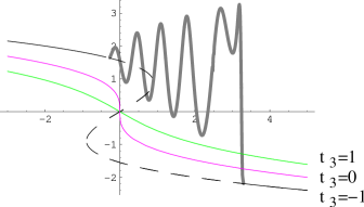
Figure 3: Solutions of the hodograph for $t_{3}=-1$ (green), $0$ (red) and $1$ (black). Unphysical multivalued region (in dashed line) of the $t_{3}=-1$-graph is replaced by an oscillatory solution in heavy gray line (numerical).

8. (2,5) critical finger. A generic flow is represented by a family of critical fingers of the form (3) with $2\ell+1=5$

$$y^{2}=(x-u)(x-d_{+})^{2}(x-d_{-})^{2}.$$ (8)

The $x^{4}$-term, and therefore $t_{5}$ in (6), can always be eliminated by a shift ($2d_{+}+2d_{-}+u=0$), leaving $t_{3}$ as the only deformation parameter. Substituting this to (6) we obtain the hodograph solution hodograph ; hodographnote

$$\frac{5}{8}\,u^{3}+\frac{3}{2}\,ut_{3}+t_{1}=0,$$ (9)

implicitly giving the branch point $u$ in terms of $t_{1}$, $t_{3}$.
A singularity occurs when $u$ merges with one or two double points $d_{\pm}=\frac{1}{4}(-u\pm\sqrt{-24t_{3}-5u^{2}})$.

The features of finger’s evolution crucially depend on the sign of $t_{3}$ (Fig. 3). If $t_{3}>0$, then the double points never reach the real axis. The function $u(t_{1})$ is single-valued and in both extraction and injection processes the finger never becomes singular (inset $\alpha$ in Fig.2).

In the case $t_{3}=0$ the solution is $u(t)\propto-(Q(t-t_{c}))^{1/3}$. This corresponds to a finger which evolves into the $(2,5)$-cusp $y^{2}=x^{5}$. At $t=t_{c}$, all the three roots coincide: $u=d_{+}=d_{-}=0$. An interesting feature of the (2,5) cusp (and of all cusps $(2,2\ell+1)$ at even $\ell$) first noted in Howison is that the evolution can be extended beyond the cusp by means of the same hodograph equation (9).

The most interesting case is $t_{3}<0$. A formal solution in the injection case leads to the (2,3)-cusp, $y^{2}\propto x^{3}$, which can not be continued. The plot in Fig. 3 becomes multi-valued in the region $t_{1}^{2}<\frac{4}{5}(-t_{3})^{3}$.

9. Air extraction – bubble break-off. We treat air extraction, where $Q<0$, and the physical time is $-t_{1}$. At an early stage, the finger tip is far to the left ($u$ is large negative and $t_{1}$ is large positive). Extracting air from the bubble results in a tip motion from left to right and a changing shape of the finger in accordance with the hodograph solution. The evolution follows the branch of the plot from $t_{1}=-\infty$ until the point $A$ in Fig. 2. At this stage, the double points $d_{\pm}$ of the curve (8) are complex. At $t_{1}=t_{A}\equiv\sqrt{{54}/{5}}\,(-t_{3})^{3/2}$ they approach the real axis and merge. As $t_{1}\to t_{A}$, the finger develops a thin neck around the point $-u/4$, which breaks at $t_{1}=t_{A}$ through the (2,4) cusp $y^{2}\propto x^{4}$. At the break-off the curve is $y^{2}=(x-u)(x+\frac{1}{4}u)^{4}$ ($u$ is negative). The bubble which breaks off from the main one has area $\frac{25\sqrt{5}}{84}(-u)^{7/2}$. After this singular point, the evolution according to the hodograph solution (9) is unphysical. It leads to an interface with a self-intersection point.

The actual evolution at $t_{1}<t_{A}$ does not follow the cubic parabola (9) in Fig.3. The correct extension of the solution beyond the singularity describes a small bubble breaking off from the finger tip. A physical solution describes the interface (or a spectral curve) $y^{2}=R_{5}(x)$ with $R_{5}(x)$ having only one rather than two double roots:

$$y^{2}=(x-u_{1})(x-u_{2})(x-u_{3})(x-d_{0})^{2},$$ (10)

where $d_{0}=V=\frac{1}{2}(u_{1}+u_{2}+u_{3})$. Now the height function $y(z)$ has two cuts: one small cut inside the small bubble and an infinite cut inside the finger (inset $\beta$ in Fig.2). The double point $d_{0}$ moves between them. Mathematically, this means that the complex curve is of genus 1 (an elliptic curve). Similarly to the genus-0 case (8), a substitution (10) into (6) we obtain

$$12t_{1}=U_{1}^{3}-4U_{3}\,,\quad-12t_{3}=U_{1}^{2}+2U_{2},$$ (11)

where $U_{k}=u_{1}^{k}+u_{2}^{k}+u_{3}^{k}$.

In case of two bubbles, $t_{1}$, $t_{3}$ are not enough to fix the dynamics. An additional conserved quantity follows from the condition on pressure. Since air is under the same pressure in both bubbles, we write $\int_{u_{2}}^{u_{3}}dp=2{\rm Re}\,\int_{u_{2}}^{u_{3}}\partial_{z}p\,dz=0$, or, using (5), ${\rm Im}\,\int_{u_{2}}^{u_{3}}\partial_{t}h^{(-)}dz=0$. Since $h^{(-)}(u_{i})=y(u_{i})=0$, we rewrite this condition as $\partial_{t}\left({\rm Im}\,\int_{u_{2}}^{u_{3}}\sqrt{R_{5}(x)}\,\,dx\right)=0$. The quantity under the integral is purely imaginary and vanishes at $t_{1}=t_{A}$, hence

$$\int_{u_{2}}^{u_{3}}\sqrt{R_{5}(x)}\,\,dx=0.$$ (12)

This condition closes the system of equations (11) after the break-off. However, unlike the algebraic equations for $t_{k}$, this condition is transcendental. A solution is available through elliptic functions. It gives the time dependence of functions $u_{1},\,u_{2},\,u_{3}$ plotted in Fig.2. After the break-off, the small bubble starts to evaporate and eventually disappears at $t_{1}=t_{C}=-\,\sqrt{{2}/{27}}\,(-t_{3})^{3/2}$ corresponding to the point $C$ on the plot. After that the solution switches back to the cubic parabola. The finger proceeds further without obstacles.

10. Discussion. Below we highlight our major results. We propose a novel, experimentally accessible modification of the Hele-Shaw cell, where the flow proceeds through singularities without being curbed by a surface tension. In this cell singularities of the flow are resolved by creation of new bubbles, all kept at the same constant pressure. This behavior can be seen experimentally.

The flow in such an air-permeable cell can be studied with the help of mathematical tools of soliton theory. We identified bubble break-off with the shock wave behavior of the KdV equation.

We are grateful to A.Marshakov, S.Nagel, R.Teodorescu and H.Swinney for discussions. We are particularly grateful to I.Krichever for help and contributions. P.W. and E.B. were supported by the NSF MRSEC Program under DMR-0213745 and NSF DMR-0220198. A.Z. was also supported in part by grants RFBR 03-02-17373, INTAS 03-51-6346, NSh-1999.2003.2. O.A. acknowledges support from the Israel Science Foundation (ISF) and from the German Israel Foundation (GIF).

References

- (1) For a review see D. Bensimon et al., Rev. Mod. Phys. 58 977 (1986), B. Gustafsson and A. Vasil’ev, http://www.math.kth.se/ gbjorn/BOOK2.pdf
- (2) R. Teodorescu, E. Bettelheim, O. Agam, A. Zabrodin and P. Wiegmann, Nucl. Phys. B 700 (2004) 521; Nucl. Phys. B 704 (2005) 407.
- (3) Gurevich, A. V. and Pitaevskiǐ, L. P., Sov. Phys. JETP, 38 (2), 291-297, 1974
- (4) Dubrovin B. A. and Novikov S. P., Russ. Math. Surveys 44 (6): 35-98 (1989), Potemin G. V., Russ. Math. Surveys 43 (5): 252-253 (1988).
- (5) Flaschka, H. Forest, M. G. and McLaughlin, D. W., Comm. Pure. Appl. Math., 33, 739-784, 1980
- (6) Singular Limit of Dispersive Waves, eds. N.M.Ercolani et al, Plenum Press, New York (1994)
- (7) Whitham, G. B., Nonlinear Dispersive Waves, SIAM Journal Appl. Math, 14 (4), 956–958, 1966
- (8) I. Krichever, M. Mineev-Weinstein, P. Wiegmann and A. Zabrodin, Physica D 198 1-28 (2004)
- (9) R. Teodorescu, A. Zabrodin and P. Wiegmann, Phys. Rev. Lett. Phys. Rev. Lett. 95 044502 (2005)
- (10) The concept of an evolving Riemann surface can be traced back to Richardson R , who related the Hele-Shaw problem to quadrature domains. The latter were then related to algebraic Riemann surfaces Quadratures1 ; Quadratures2 , while a direct application of this theory was made in Quadratures3
- (11) S. Richardson, J. Fluid Mech. 56 609 (1972)
- (12) D. Aharonov and H. S. Shapiro, J. Anal. Math. 30 (1976), 39
- (13) B. Gustafsson, Acta Appl. Math. 1 (1983), 209
- (14) D. Crowdy and H. Kang , Journal of NonLinear Science, 11 (2001), 279
- (15) Novikov, S., Manakov, S. V. and Pitaevskiǐ, L. P. and Zakharov, V.E,Theory of Solitons: The Inverse Scattering Method, Consultants Bureau, New-York and London, 1984
- (16) S. P. Tsarev, Soviet Math. Dokl., 31, 488, 1985, Krichever, I. M., Functional Analysis and its Applications, 22 (3), 200-213, 1988
- (17) The general hodograph equation reads .
- (18) S. Howison, SIAM J. Appl. Math. 46 20 (1986)