Dynamic characterisers of spatiotemporal intermittency

Abstract

We study spatiotemporal intermittency in a system of coupled sine circle maps. The phase diagram of the system shows parameter regimes where the STI lies in the directed percolation class, as well as regimes which show pure spatial intermittency (where the temporal behaviour is regular) which do not belong to the DP class. Thus, both DP and non-DP behaviour can be seen in the same system. The signature of DP and non-DP behaviour can be seen in the dynamic characterisers, viz. the spectrum of eigenvalues of the linear stability matrix of the evolution equation, as well as in the multifractal spectrum of the eigenvalue distribution. The eigenvalue spectrum of the system in the DP regimes is continuous, whereas it shows evidence of level repulsion in the form of gaps in the spectrum in the non-DP regime. The multifractal spectrum of the eigenvalue distribution also shows the signature of DP and non-DP behaviour. These results have implications for the manner in which correlations build up in extended systems.

I Introduction

The phenomenon of spatiotemporal intermittency (STI), which is characterized by the coexistence of laminar states of regular dynamics, and burst states of irregular dynamics, is ubiquitous in natural and experimental systems. Such behaviour has been seen in experiments on convection cili ; daviaud , counterrotating Taylor-Couette flow colo , oscillating ferro-fluidic spikes rupp , and experimental and numerical studies of rheological fluids sriram ; fielding . In theoretical studies, STI has been seen in PDEs such as the damped Kuramoto-Sivashinsky equation kschate and the one-dimensional Ginzburg Landau equation glchate , coupled map lattices kaneko such as the Chaté-Manneville CML Chate , the inhomogeneously coupled logistic map lattice ash , and in cellular automata studies Chate .
A variety of scaling laws have been observed in these systems. However, there are no definite conclusions about their universal behaviour. Many of the observed phenomena have been seen in experimental systems where no simple model is available. There has been much discussion about the nature of spatiotemporal intermittency and its analogy with systems which undergo phase transitions. It has been argued that the transition to spatiotemporal intermittency with absorbing laminar states is a second order phase transition, and that this transition falls in the same universality class as directed percolation Pomeau with the laminar states being identified with the ‘inactive’ states and the turbulent states being identified as the ‘active’ or percolating states. This conjecture has become the central issue in a long-standing debate Rolf ; Chate ; Houlrik ; Grassberger ; Janaki , which is still not completely resolved. Thus, the analysis of spatiotemporal intermittency remains a challenging theoretical problem.

In this paper, we study spatiotemporal intermittency in the coupled sine circle map lattice Nandini , a popular model for the behaviour of mode-locked oscillators. Spatiotemporal intermittency has been reported to exist for several points in the parameter space of this model and a full set of directed percolation exponents has been found at these points Janaki ; Zahera . The detailed phase diagram of this model shows that these points lie on, or near, the bifurcation boundary where the synchronized fixed points of the model lose stability. We now find that spatiotemporal intermittency can be found all along the bifurcation boundary of this region. Interestingly, while some points of this boundary show spatiotemporal intermittency where synchronized laminar regions coexist with turbulent regions, with associated directed percolation exponents (DP), other points of the boundary show pure spatial intermittency where the synchronized laminar regions are interspersed with bursts of temporally periodic or quasi-periodic behaviour which are not associated with DP exponents.Thus, both DP and non-DP regimes can be seen in this model. The distinct signatures of these two types of behaviour can be found in the eigenvalue distribution of the stability matrix calculated at one time step. The eigenvalue spectrum of the system in the DP regimes is continuous, whereas distinct gaps can be seen in the spectrum in the non-DP regime. The multifractal analysis of the eigenvalue distribution of the two cases also shows the signature of this behaviour. Thus, the signature of the DP and non-DP behaviour of the model can be found in the dynamic characterisers of the system. In the case of low dimensional systems, intermittency of different types has been observed to contribute characteristic signatures to the distribution of finite time Lyapunov exponents Ram . The present study indicates the presence of a similar phenomenon in high-dimensional systems as well.

The organisation of this paper is as follows. The details of the model are given in section II. The phase diagram of this CML is discussed in the same section and the various types of STI observed are described therein. In section III, the universality classes are identified and the differences between the STI belonging to the DP class and non-DP classes are quantified. Section IV describes dynamic characterisers which can pick up these distinct classes. The paper ends with a discussion of these results.

II The Model and the phase diagram

The coupled sine circle map lattice has been known to model the mode-locking behaviour gauri2 seen commonly in coupled oscillators, Josephson Junction arrays, etc, and is also found to be amenable to analytical studies Nandini . The model is defined by the evolution equations

$$x_{i}^{t+1}=(1-\epsilon)f(x_{i}^{t})+\frac{\epsilon}{2}[f(x_{i-1}^{t})+f(x_{i+1}^{t})]\pmod{1}$$ (1)

where $i$ and $t$ are the discrete site and time indices respectively and $\epsilon$ is the strength of the coupling between the site $i$ and its two nearest neighbours. The local on-site map, $f(x)$ is the sine circle map defined as

$$f(x)=x+\Omega-\frac{K}{2\pi}\sin(2\pi x)$$ (2)

Here, $K$ is the strength of the nonlinearity and $\Omega$ is the winding number of the single sine circle map in the absence of the nonlinearity. We study the system with periodic boundary conditions in the parameter regime $0<\Omega<\frac{1}{2\pi}$ (where the single circle map has temporal period 1 solutions), $0<\epsilon<1$ and $K=1.0$. The phase diagram of the system is highly sensitive to initial conditions due to the presence of many degrees of freedom and has been studied extensively for several classes of initial conditions Nandini ; gauri2 , which result in rich phase diagrams with many distinct types of attractors. In particular, this system has regimes of spatiotemporal intermittency (STI) when evolved in parallel with random initial conditions Janaki . An earlier study of the inhomogeneous logistic map lattice had shown that the bifurcation curves corresponding to bifurcations from the synchronized fixed point, can form rough guide-lines to the regions in parameter space where STI can be found ash . It is therefore worthwhile to investigate the detailed phase-diagram of the present system, identify various types of dynamical behaviour, and correlate the observed behaviour, especially the spatiotemporally intermittent behaviour, with the known bifurcations that occur in the system.

II.1 The Phase Diagram

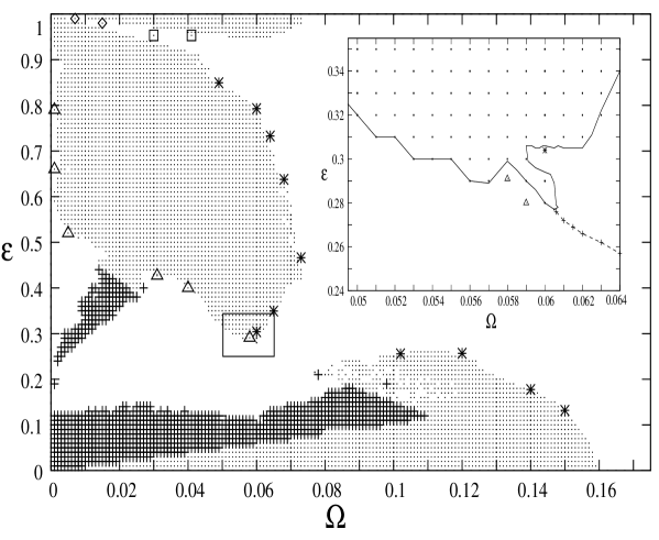
Figure 1: shows the phase diagram obtained at $K=1.0$ for a lattice of size $N=1000$. A transient of 15000 iterates has been discarded. The dots represent the synchronized fixed point solutions. Plus ($+$) signs represent the cluster solutions. The diamonds ($\Diamond$) represent STI with traveling (TW) wave laminar states and turbulent bursts whereas boxes ($\Box$) represent STI with TW laminar state and turbulent bursts containing solitons. The asterisks ($\ast$) represent STI belonging to the DP class, and spatial intermittency is represented by triangles ($\triangle$). The crossover regime from spatial intermittency to DP is magnified in the inset figure. SI with frozen bursts are seen below the dashed line. Above this line, the bursts start spreading on the lattice.

The phase diagram of the system of Eqs. 1 and 2 for the parameter region mentioned above is shown in Fig. 1. Many types of solution can be seen in the phase diagram. Stable, synchronized, fixed point solutions, where the variables $x_{i}$ take the value, $x_{i}^{t}=\frac{1}{2\pi}\sin^{-1}(\frac{2\pi\Omega}{K})=x^{\star}$ for all $i=1,\ldots N$ for all $t$, are indicated by dots. These solutions, which are very robust against perturbations, can be seen in large regions of the phase diagram. Cluster solutions, in which $x_{i}^{t}=x_{j}^{t}$ for $i,j$ belonging to the same cluster are also seen in the phase diagram, and are indicated by $+$ signs in Fig. 1. The synchronized solution is, in fact, a single cluster solution where the size of the cluster is the lattice itself. Spatiotemporally intermittent solutions are seen near the bifurcation boundaries where these synchronized solutions lose stability. Several distinct kinds of STI are seen in the phase diagram. These are:

(a)	(b)
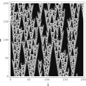
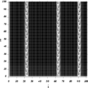
(c)	(d)

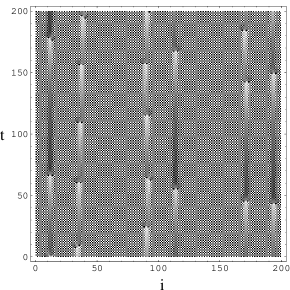
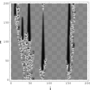
Figure 2: shows the space time plots of the different types of STI observed in the phase diagram. The lattice index $i$ is along the x-axis and the time index $t$ is along the y-axis. The space time plots show (a) STI with synchronized laminar state interspersed with turbulent bursts seen at $\Omega=0.06,\epsilon=0.7928$. (b) SI with synchronized laminar state with quasiperiodic and periodic bursts seen at $\Omega=0.031,\epsilon=0.42$. (c) STI with TW laminar state and turbulent bursts observed at $\Omega=0.007,\epsilon=0.99$. (d) STI with TW laminar state and turbulent bursts containing solitons at $\Omega=0.03,\epsilon=0.954$.

1. STI where the synchronized laminar state is interspersed with turbulent bursts is seen along the bifurcation boundary starting from $\Omega=0.0457,\epsilon=0.89$ to $\Omega=0.06,\epsilon=0.30396$. Some of the points where this kind of STI is seen are shown by asterisks ($\ast$) in the phase diagram. The laminar state corresponds to the synchronized fixed point $x^{\star}$ defined earlier. The turbulent state takes all values other than $x^{\star}$ in the [0,1] interval. The space-time plot of these solutions is shown in Fig. 2(a).

2. Spatial intermittency (SI) with a synchronized laminar state interspersed with quasi-periodic and periodic bursts is seen along the boundary marked by triangles ($\triangle$) in the phase diagram. (The triangles indicate specific locations where the SI has been studied). The laminar state is the synchronized fixed point $x^{\star}$ and the burst state is a mixture of quasi-periodic and periodic bursts. (See Fig. 2(b)).

3. The locations where STI with travelling wave laminar states and turbulent bursts can be seen are marked by diamonds ($\Diamond$) in the phase diagram (Fig. 2(c)). As can be seen from the space-time plot, the burst states are localized and do not spread through the lattice.

4. Parameter values which show spatiotemporal intermittency with travelling wave laminar states and turbulent bursts are shown by boxes ($\Box$) in the phase diagram. The space-time plot of such states can be seen in Fig. 2(d). These states differ from those seen in Fig. 2(c) in that apart from the turbulent bursts, soliton-like structures which are turbulence of a coherent nature traveling in space and time, are also seen in this type of STI. Such coherent structures have also been seen in the Chaté-Manneville class of CMLs Grassberger ; bohr .

We concentrate on STI with the simplest version of the laminar state, viz. the synchronized state. Two types of intermittent behaviour are associated with this laminar state, viz. spatiotemporal intermittency with spreading turbulent bursts, and spatial intermittency with localised periodic and quasi-periodic bursts. These two types of behaviour can be seen in contiguous regions of the boundary, but belong to different universality classes. We discuss this behaviour below, as well as the cross-over region between the two types of behaviour. STI with other types of laminar states, as well as STI in the presence of solitons will be dealt with elsewhere. The blank regions of the phase diagram show solutions of varying degrees of spatiotemporal irregularity which will also be discussed elsewhere.

III Universality classes in Spatiotemporal Intermittency

We contrast the two types of intermittency and identify their universality classes in this section. It is seen that spatiotemporal intermittency with spreading bursts belongs to the directed percolation class, whereas spatial intermittency with periodic/quasi-periodic bursts does not belong to the directed percolation class. The signature of this behaviour can be seen in the dynamic characterisers of the system, viz. the distribution of eigenvalues of the linear stability matrix.

III.1 STI of the Directed Percolation class

The phase diagram shows STI with synchronized laminar state interspersed with turbulent bursts along the upper boundary of the leaf shaped region where synchronized solutions are stable (the boundary on which asterisks are seen). These solutions show spreading and infective behaviour similar to that seen in directed percolation models stauffer . In this type of STI, the spontaneous creation of turbulent bursts does not take place as can be seen in the space-time plot of this STI (Fig. 2(a)). A laminar site becomes turbulent only if it has been infected by a neighbouring turbulent site at the previous time-step. The turbulence either spreads to the whole lattice, or dies down completely to the laminar state depending on the coupling strength, $\epsilon$. Once all the sites in the lattice relax to the laminar state, it remains in this state forever. Hence, the synchronized laminar state is the absorbing state. Importantly, this type of STI, as seen in this model, is free of solitons which could bring in long-range correlations. Hence, a straightforward analogy with the DP class can be drawn in this case, where the burst states are identified with the ’wet’ sites, the laminar states are the ’dry’ sites and the time axis acts as the directed axis.

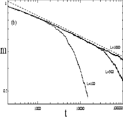
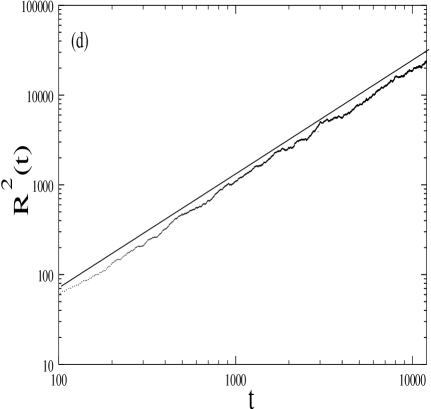
Figure 3: (a) shows the log-log plot of the escape time, $\tau$ vs lattice size $L$ at $\Omega=0.049$ and $\epsilon=0.852,0.8498,0.8495,0.8492,0.849$ from top to bottom. At $\epsilon_{c}=0.8495$, $\tau$ scales with $L$ with $z=1.60\pm 0.01$. (b) shows the log-log plot of order parameter, $m$ vs $t$ at $\Omega=0.073,\epsilon=0.4664$. The exponent $\beta/{\nu z}=0.157$. (c) shows the log-log plot of the correlation function $C_{j}(t)$ vs $j$ at $\Omega=0.049,\epsilon=0.8495$ at timesteps $t=65000,35000,15000$ shown as $\Diamond,+,\times$ respectively. The exponent $\eta^{\prime}-1=0.51$ (d) shows the log-log plot of the radius of gyration, $R^{2}(t)$ vs $t$ at $\Omega=0.073,\epsilon=0.4664$. $z_{s}=1.268$. All logarithms are to base 10.

The DP transition is characterised by a set of static critical exponents associated with physical quantities of interest such as the escape time, the order parameter which is defined as the fraction of turbulent sites in the lattice at time $t$, the distribution of laminar lengths, and the pair correlation function. In addition, a set of dynamic critical exponents can be obtained by considering temporal evolution from initial conditions which correspond to an absorbing background with a localised disturbance, i.e. a few contiguous sites which are different from an absorbing background. The quantities of interest are, the time dependence of $N(t)$, the number of active sites at time $t$ averaged over all runs, $P(t)$, the survival probability, or the fraction of initial conditions which show a non-zero number of active sites (or a propagating disturbance) at time $t$ and the radius of gyration $R^{2}(t)$, which is defined as the mean squared deviation of position of the active sites from the original sites of the turbulent activity, averaged over the surviving runs alone. The detailed definition of the full set of DP exponents is given in the appendix and typical behaviour is shown in Fig. 3. This complete set of DP exponents has been calculated at the points marked by asterisks in the phase diagram (Fig. 1). (The exponents at two of these points viz. at parameters $\Omega=0.068,\epsilon=0.63775$, $K=1.0$, and $\Omega=0.064,\epsilon=0.73277$, $K=1.0$ were found in an earlier work Janaki ).

$\Omega$	$\epsilon_{c}(\Omega)$	Bulk exponents
		$z$	$\beta/{\nu z}$	$\beta$	$\nu$	$\eta^{\prime}$	$\zeta$	$\zeta^{\prime}$
0.049	0.8495	1.60$\pm$.01	0.16$\pm$0.01	0.271	1.1	1.51$\pm$0.0	1.68$\pm$0.01	0.87$\pm$0.01
0.06	0.7928	1.59$\pm$0.02	0.17$\pm$0.02	0.293	1.1	1.51$\pm$0.01	1.68$\pm$0.01	0.78$\pm$0.01
0.073	0.4664	1.58$\pm$0.02	0.16$\pm$0.01	0.273	1.1	1.5$\pm$0.01	1.65$\pm$0.01	0.72$\pm$0.01
0.065	0.34949	1.59$\pm$0.03	0.16$\pm$0.01	0.273	1.1	1.5$\pm$0.01	1.66$\pm$0.01	0.75$\pm$0.01
0.06	0.30396	1.6$\pm$0.02	0.16$\pm$0.01	0.27	1.05	1.5$\pm$0.01	1.61$\pm$0.01	0.70$\pm$0.01
0.102	0.25554	1.6$\pm$0.01	0.16$\pm$0.00	0.277	1.1	1.52$\pm$0.01	1.67$\pm$0.01	0.73$\pm$0.01
0.12	0.257	1.60$\pm$0.01	0.15$\pm$0.01	0.264	1.1	1.51$\pm$0.01	1.64$\pm$0.01	0.71$\pm$0.01
DP		1.58	0.16	0.28	1.1	1.51	1.67	0.748

Table 1: The static exponents obtained at the critical $\epsilon_{c}$ are shown in the above table. The universal DP exponents are listed in the last row. These exponents have been obtained after averaging over 1000 initial conditions.

$\Omega$	$\epsilon_{c}$	Spreading Exponents
		$\eta$	$\delta$	$z_{s}$
0.049	0.8495	0.308$\pm$0.002	0.17$\pm$0.02	1.26$\pm$0.01
0.06	0.7928	0.315$\pm$0.007	0.16$\pm$0.01	1.26$\pm$0.01
0.073	0.4664	0.308$\pm$0.001	0.17$\pm$0.01	1.27$\pm$0.00
0.065	0.34949	0.303$\pm$0.001	0.16$\pm$0.01	1.27$\pm$0.01
0.06	0.30396	0.317$\pm$0.001	0.17$\pm$0.01	1.26$\pm$0.0
0.102	0.25554	0.315$\pm$0.001	0.16$\pm$0.00	1.25$\pm$0.01
0.12	0.257	0.305$\pm$0.00	0.16$\pm$0.00	1.27$\pm$0.03
DP		0.313	0.16	1.26

Table 2: The spreading exponents obtained at $\epsilon_{c}$ are shown in the above table. The last row lists the DP exponents.

All these points are located near the bifurcation boundary of the spatiotemporally synchronized solutions. The static and dynamic exponents obtained after averaging over $10^{3}$ initial conditions at these parameter values have been listed in Table 1 and 2 respectively. The agreement between these exponents and the universal DP exponents is complete.

III.2 Spatial intermittency shows non-DP behaviour

Spatial intermittency with synchronized laminar state, and quasi-periodic or periodic bursts, is also seen in the vicinity of the bifurcation boundary at the locations indicated by triangles. The laminar state is the synchronized fixed point $x^{\star}$ defined earlier. The bursts observed are quasi-periodic in nature. Fig. 2(b) shows the space-time plot of SI. We can see the absence of spreading dynamics or infective behaviour on the lattice. The bursts are spatially localized which is unlike the dynamics seen in directed percolation systems. The spatially intermittent solutions have zero velocity components in the spatial direction, and modes which travel along the lattice do not appear. In addition to the solutions with quasiperiodic bursts seen in the space-time plot, solutions which have strictly periodic bursts can also be seen.

Figure 4: shows the $\log-\log$ (base 10) plot of the laminar length distribution for (a) STI with synchronized laminar state obtained at $\Omega=0.06,\epsilon=0.7928$. The exponent obtained is 1.681. (b) SI obtained at $\Omega=0.04,\epsilon=0.4$. The exponent $\zeta$ is 1.12.

The scaling exponent $\zeta$ for the laminar length distribution $P(\ell)\sim\ell^{-\zeta}$, is found to have the value $1.1$ in the case of SI which is very different from the corresponding DP exponent ($\zeta_{DP}=1.67$) (Fig. 4). Hence, SI does not belong to the DP universality class. We note that this exponent, however, has been seen for the inhomogenously coupled logistic map lattice ash where similar spatial intermittency is seen.

III.3 Cross-over Regime

It is clear from the phase diagram that the regimes of spatial intermittency and spatiotemporal intermittency are contiguous to each other on the lower part of the bifurcation boundary of the synchronized solutions ( in the neighbourhood of $\Omega=0.06$ and $\epsilon=0.3$ ), and cross-over effects can be expected in this parameter regime. This cross-over region is magnified in the inset to Fig. 1. The transition takes place through an intermediate stage wherein apart from periodic and quasi-periodic bursts, frozen bursts are also seen. This regime is found just below the dashed line shown in the inset, e.g. at $\Omega=0.0608$, $\epsilon=0.273$. Here, the laminar length distribution is exponential in nature (See Fig. 5). Above the dashed line (e.g. at $\Omega=0.061$ and $\epsilon=0.273$), the crossover starts with the appearance of bursts which spread on the lattice. As $\epsilon$ is increased further, the bursts lose their localised nature and STI with synchronized laminar state is seen. At the point marked by an asterisk ($\ast$) in the figure, DP exponents are obtained.

(a)	(c)
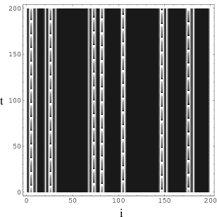
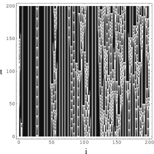
(b)	(d)

Figure 5: shows the behaviour on either side of the crossover line shown in Fig. 1 (inset). Fig 5(a) shows the space-time plot of SI seen at $\Omega=0.0608,\epsilon=0.273$. Frozen bursts can be seen in the space-time plot. The laminar length distribution is plotted on a semi-log plot (base 10) in Fig 5(b) . The fit to this distribution is $13.0~{}\exp~{}(-0.05x)$ Fig 5(c) shows the space-time plot obtained at $\Omega=0.061,\epsilon=0.273$. The laminar length distribution is shown in Fig 5(d). The fit is $12.06~{}\exp~{}(-0.043x)$

The distinction between the DP and non-DP regimes lies in the extent to which the burst solutions are able to spread into the laminar regions, i.e. the extent to which they are able to infect the laminar regions. While the spreading exponents are the obvious signature to this problem, their non-universal nature, and strong dependence on the initial configuration makes their use problematic. However, the dynamic signature of the extent to which burst solutions can spread and mix into the laminar regions, is contained in the spectrum of the eigenvalue distribution of the one-step stability matrix and also in the multifractal spectrum of the eigenvalue distribution. The eigenvalue spectrum of the DP class is continuous whereas the non-DP class contains distinct gaps in the spectrum indicating regions where the eigenvalues are repelled, corresponding to stretching rates which are excluded. These gaps appear to lead to the strong spatial localisation and temporally regular/quasi-regular behaviour for the burst solutions characteristic of spatial intermittency. The multifractal spectrum of the eigenvalues also contains the signature of this behaviour. Thus, the eigenvalue spectrum and the multifractal spectrum of the eigenvalues, constitute dynamic characterisers of spatiotemporal intermittency. We elaborate on these characterisers in the next section.

IV Dynamic signatures of DP and non-DP class

IV.1 The eigenvalue distribution of the stability matrix

The linear stability matrix of the evolution equation 1 at one time-step about the solution of interest is given by the $N\times N$ dimensional matrix, $M_{t}^{N}$, given below

$$\mathbf{M_{t}^{N}}=\left(\begin{array}[]{ccccc}\epsilon_{s}f^{\prime}(x_{1}^{t})&\epsilon_{n}f^{\prime}(x_{2}^{t})&0&\ldots&\epsilon_{n}f^{\prime}(x_{N}^{t})\\ \epsilon_{n}f^{\prime}(x_{1}^{t})&\epsilon_{s}f^{\prime}(x_{2}^{t})&\epsilon_{n}f^{\prime}(x_{3}^{t})&\ldots&0\\ 0&\epsilon_{n}f^{\prime}(x_{2}^{t})&\epsilon_{s}f^{\prime}(x_{3}^{t})&\epsilon_{n}f^{\prime}(x_{4}^{t})&\ldots\\ \vdots&\vdots&\vdots&\vdots&\vdots\\ \epsilon_{n}f^{\prime}(x_{1}^{t})&0&\ldots&\epsilon_{n}f^{\prime}(x_{N-1}^{t})&\epsilon_{s}f^{\prime}(x_{N}^{t})\\ \end{array}\right)$$

where, $\epsilon_{s}=1-\epsilon$, $\epsilon_{n}=\epsilon/2$, and $f^{\prime}(x_{i}^{t})=1-K\cos(2\pi x_{i}^{t})$. $x_{i}^{t}$ is the state variable at site $i$ at time $t$, and a lattice of $N$ sites is considered.

The diagonalisation of $M^{N}_{t}$ gives the $N$ eigenvalues of the stability matrix. The eigenvalues of the stability matrix were calculated for spatiotemporally intermittent solutions which result from bifurcations from the spatiotemporally synchronized solutions. The eigenvalue distribution for the STI belonging to the DP universality class and SI was calculated by averaging over 50 initial conditions.

The eigenvalue distributions for STI belonging to the DP class can be seen in the Fig. 6(a), and that for spatial intermittency can be seen in Fig. 6(b). It is clear from the insets, the eigenvalue spectrum of the SI case shows distinct gaps. No such gaps are seen in the eigenvalue spectrum of the STI belonging to the DP class and the spectrum is continuous. Thus, a form of level repulsion is seen in the eigenvalue distribution for parameter values which show spatial intermittency. We note that such gaps are seen at all the parameter values studied where spatial intermittency is seen, and that no gaps are seen for any of the parameter values where DP is seen FN . It can be seen that 6(c) shows power-law scaling (with power $-1.254$) in the range $0.1$ to $1$ unlike Fig. 6(d). The gaps in the spectrum can also be seen in Fig. 6(d). Thus, the gaps in the spectrum are associated with temporally quasi-periodic or periodic bursts in a synchronized fixed point laminar background. The bursts have no velocity component along the lattice, and hence do not travel in space, nor do they infect their laminar neighbours. On the other hand, when the spectrum is continuous the bursts are temporally turbulent and show the infective behaviour characteristic of

Figure 6: shows the eigenvalue distribution for (a) STI belonging to the DP class at $\Omega=0.06,\epsilon=0.7928$ and (b) Spatial intermittency at $\Omega=0.04,\epsilon=0.4$. A section of the eigenvalue distribution is magnified in the inset figures. Gaps are seen in the spatial intermittency eigenvalue distribution whereas the eigenvalue distribution for STI does not show any such gaps. The logarithmic plots (base 10) of $P(\lambda)$ versus $\lambda$ can be seen in Fig. 6(c) for the DP class (for the positive part of the spectrum) and Fig. 6(d) for the spatial intermittency.

directed percolation problems. Since the eigenvalue spectrum of the SI case has zero probability regions, they are strongly picked up by multifractal analysis. However, it is interesting to note that the multifractal analysis of this case, with gaps excluded, also carries the signature of spatial intermittency. We discuss these signatures in the next section.

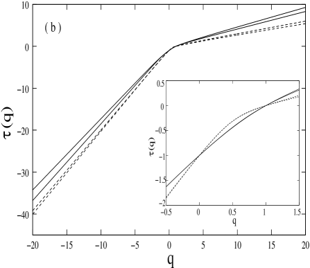
Figure 7: (a) shows the $\tau(q)$ vs $q$ curves for $\Omega=0.058,\epsilon=0.291$ including the gaps (solid line) and excluding the gaps (dashed line); (b) shows the $\tau(q)$ vs $q$ curves (with gaps excluded) for $\Omega=0.073,\epsilon=0.4664$; $\Omega=0.06,\epsilon=0.30396$; $\Omega=0.058,\epsilon=0.291$ and $\Omega=0.04,\epsilon=0.4$ from top to bottom. The first two curves represent STI belonging to the DP class (shown by solid lines) and the last two represent spatial intermittency. The difference in the curvatures of $\tau(q)$ for the DP and the non-DP class can be seen in the inset figure in which the region near $q=0.0$ has been magnified.

IV.2 Multifractal Analysis

The eigenvalue distributions obtained at different parameter values were analysed using the multifractal framework halsey ; rang . Given a probability distribution whose support is covered by equal lengths, the generalized dimensions, $D_{q}$, are defined by the relation

$$D_{q}=\frac{1}{q-1}~{}\lim_{l\rightarrow 0}~{}~{}\frac{\log\sum_{i}p_{i}^{q}}{\log l}$$ (3)

where $p_{i}$ is the probability associated with the $i^{th}$ bin and $l$ is the bin-size. Clearly, $D_{q}$ picks out the effect of larger probabilities at large positive $q$’s and smaller probabilities at large negative $q$’s. The quantity $\tau(q)$ is defined as

$$\tau(q)=D_{q}(q-1)$$ (4)

The $\tau(q)$ vs $q$ spectrum for the STI and SI cases are shown in Fig. 7. Fig. 7(a) has been plotted for the parameter values $\Omega=0.058,\epsilon=0.291$, where spatial intermittency is seen, and there are gaps in the spectrum. The solid line is the plot of $\tau$ versus $q$ for the case where the entire support of the distribution is covered with equal lengths of $s=0.005$. It is clear that $\tau(q)$ diverges to $-\infty$ for negative values of $q$, due to the presence of gaps in the spectrum where the distribution takes zero values.

The dotted line in Fig. 7(a) corresponds to the $\tau$ versus $q$ curve obtained for the same distribution without including the contribution of the gaps. While the $\tau(q)$ now no longer diverges, its behaviour is still distinct from that obtained from the distributions which correspond to DP regimes. This can be seen in Fig. 7(b). We see that the $\tau(q)$ curves show different behaviour in the neighbourhood of $q=0$ for the DP(solid lines) and non-DP (dotted lines) cases. The behaviour in the vicinity of the knee of the curve is magnified and shown in the inset. The dotted lines corresponding to the SI case fall on the same curve here, and are distinct from the curve on which the solid lines of the DP case fall (although both sets of curves separate out for large values of $|q|$). It is clear that the curvature of the $\tau$ versus $q$ curve in this region is different near $q=0$ for the DP and non-DP cases. The curvature of $\tau(q)$, $\frac{d^{2}\tau(q)}{dq^{2}}$ for the two types of STI is shown in Fig. 8. The negative and positive parts of the y-axis have been interchanged for ease of representation. A twin peak is seen in the curvature of $\tau(q)$ of STI belonging to the DP class (Fig. 8(a)) whereas a single peak is seen in the case of spatial intermittency (Fig.8(b)). Fig. 8(c) shows the curvature of the SI case, for $q$ positive, with gaps included (solid line), and gaps excluded ($\Diamond$). A jump is seen in the spectrum at $q=0.0$ due to the contribution of the gaps, and the two curvatures coincide completely for $q$ positive.
The signatures of the $DP$ versus non-DP behaviour can also be seen in the $f-\alpha$ curves of the distribution. The $\alpha(q)$, the scaling exponent of the probabilities, and $f(\alpha)$, the fractal dimension of the set which supports the probability which scales with the exponent $\alpha$, are obtained from the relations $\alpha(q)=\frac{d\tau(q)}{dq}$ and $f(\alpha)=q\alpha(q)-\tau(q)$. The $f(\alpha)$ vs $\alpha$ spectra of the STI and SI cases are plotted in Figs 9(a) and 9(b) respectively (where the SI regime has been analysed omitting the gaps in the spectrum). It is clear that STI of the DP class shows $f-\alpha$ behaviour distinct from the SI class. The SI curves are more asymmetric and peak at higher values of $\alpha$. It is also interesting to note that STI of the DP class at distinct parameter values collapse quite closely on the same $f-\alpha$ curve for positive $q$ (since $\frac{df}{d\alpha}=q$, this is the part of the curve with positive slope), but separate out for negative $q-s$, whereas the data for the SI case does not fall on the same curve for either regime.

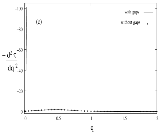
Figure 8: shows $-\frac{d^{2}\tau(q)}{dq^{2}}$ plotted against $q$ for (a) STI belonging to DP class calculated at (i) $\Omega=0.073,\epsilon=0.4664$ and (ii) $\Omega=0.06,\epsilon=0.30396$; and for (b) spatial intermittency at parameters (i) $\Omega=0.058,\epsilon=0.291$ and (ii) $\Omega=0.031,\epsilon=0.42$. Twin peaks are seen for STI belonging to the DP class; (c) shows $-\frac{d^{2}\tau(q)}{dq^{2}}$ obtained for SI including gaps and excluding gaps. A sharp change is seen near $q=0.0$ when gaps are included.

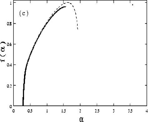
Figure 9: shows the $f(\alpha)$ vs $\alpha$ curves for (a) STI belonging to the DP class at parameters ($\Omega=0.06,\epsilon=0.7928$), ($\Omega=0.064,\epsilon=0.73277$), ( $\Omega=0.073,\epsilon=0.4664$) labelled as 1,2,3 respectively in Fig. (a) and; (b) Spatial Intermittency at parameters ($\Omega=0.031,\epsilon=0.42$), ( $\Omega=0.04,\epsilon=0.4$) and ($\Omega=0.058,\epsilon=.291$) labelled as 1, 2, and 3 respectively in Fig.(b). The $f(\alpha)$ spectrum for the DP class (Fig.(a) overlap with each other for small positive $q$’s whereas the $f(\alpha)$ curves for SI class (Fig.(b)) do not coincide with those of the DP class; (c) shows the $f(\alpha)$ curve obtained with gaps ($\Diamond$) and without gaps (line).

Fig. 9(c) shows the comparison between the $f-\alpha$ spectrum of the SI distribution with gaps excluded (dotted line), and that where the gaps are included (diamonds, plotted for positive $q-s$, only). The contribution of the gaps can be very clearly seen. We also note that cross-over effects can be seen in the dynamical characterisers as well, and the distributions cross over from those characteristic of DP behaviour, to those characteristic of non-DP behaviour.

Thus, the absence or presence of the gaps in the eigenvalue spectrum constitutes the primary signature of DP and non-DP behaviour in this system. The leading signature of DP or non-DP behaviour in the multifractal spectrum is the divergence of the $\tau$ versus $q$ curve for negative $q-s$, as well as corresponding behaviour in the $f-\alpha$ spectrum. However, the secondary signatures of DP versus non-DP behaviour can be found even when the $\tau$ versus $q$ for SI is obtained excluding the gaps which contribute to the divergence in the curvature of the $\tau$ versus $q$ curve. Thus, the distribution of eigenvalues of the stability matrix and the multifractal spectrum of the distribution constitute the dynamic characterisers of DP and non DP behaviour.

V Discussion

To summarise, the phase diagram of the coupled sine circle map shows regimes of spatiotemporal intermittency of different types. The regimes of spatiotemporal intermittency with synchronized laminar states and turbulent bursts are characterised by a complete set of DP exponents. Regimes of spatial intermittency, where the bursts have regular temporal behaviour, do not show infective behaviour, and do not belong to the DP class. Thus the same model can show DP and non-DP behaviour in different regions of the parameter space. The signature of the DP and non-DP behaviour can be seen in the dynamical characterisers of the system, viz. the distribution of eigenvalues and the multifractal spectrum of this distribution. Gaps in the eigenvalue spectrum are characteristic of spatial intermittency, i.e. of spatially localised, temporally regular or quasi-regular bursts with associated non-DP exponents. The eigenvalue spectrum is continuous for regimes of regular spatiotemporal intermittency with spreading bursts and characteristic DP exponents. The model also shows spatiotemporally intermittent regimes with other types of laminar and burst states. The scaling behaviour in these regimes, and the identification of their universality classes is being pursued further. In order to gain insight into the way in which correlations build up in this system, it may be useful to set up probabilistic cellular automata which exhibit similar regimes and to examine their associated spin Hamiltonians Domany . The comparison of the scaling exponents seen in this model with those seen in absorbing phase transitions which do not belong to the DP class chatepmpm ; chatepmpm1 ; chatejk ; hinrich1 ; odor1 is also of interest. We hope to examine some of these questions in future work.

VI Acknowledgement

NG thanks BRNS, India for partial support. ZJ thanks CSIR for financial support.

Appendix A The definition of dp exponents

The DP transition is characterised by a set of static and dynamic critical exponents associated with various quantities of physical interest.

A.1 Static exponents

1. We first consider the escape time $\tau(\Omega,\epsilon,L)$, which is defined as the time taken for the system starting from random initial conditions to relax to a completely laminar state. It is expected from finite-size scaling arguments that $\tau$ varies with the system size $L$ such that

   $$\tau(\Omega,\epsilon)=\left\{\begin{array}[]{ll}\log L&\textrm{Laminar phase}\\ L^{z}&\textrm{Critical phase}\\ \exp L^{c}&\textrm{Turbulent phase}\end{array}\right.$$

   Hence, at the critical value of the coupling strength, $\epsilon_{c}$, the escape time $\tau$ shows a power law behaviour, $z$ being the associated exponent.

2. The order parameter $m(t)$, associated with this transition is defined as the fraction of turbulent sites in the lattice at time $t$. At $\epsilon_{c}$, the order parameter scales as

   $$m\sim(\epsilon-\epsilon_{c})^{\beta},~{}~{}~{}\epsilon\rightarrow\epsilon^{+}$$ (5)

   At $t<<\tau$, $m(t)$ scales with $t$ as $m(\epsilon_{c},t)\sim t^{-\beta/{\nu z}}$, where $\nu$ is exponent associated with the spatial correlation length.

   The exponent $\nu$ is obtained by using the scaling relation

   $$\tau(L,\epsilon_{c})\sim\phi^{z}f(L/\phi)$$ (6)

   where, $\phi$ is the correlation length which diverges as $\phi\sim\delta^{-\nu}$ and $\delta$ is given by $(\epsilon$ - $\epsilon_{c})$. Hence, $\nu$ is adjusted until the scaled variables $L\delta^{\nu}$ and $\tau\delta^{\nu z}$ collapse onto a single curve.

3. The correlation function in space is defined as

   $$C_{j}(t)=\frac{1}{L}\sum_{i=1}^{L}<x_{i}^{t}x_{i+j}^{t}>-<x_{i}^{t}>^{2}$$ (7)

   At $\epsilon_{c}$, $C_{j}(t)$ scales as $C_{j}(t)\sim j^{1-\eta^{\prime}}$.
   

4. The distribution of laminar lengths, $P(l)$ is an important characteriser of the universality class Chate . The laminar lengths, $l$ are defined as the number of laminar sites between two turbulent sites. At criticality, the laminar length distribution shows a power-law behaviour of the form

   $$P(l)\sim l^{-\zeta}$$ (8)

   $\zeta$ is the associated exponent, $\zeta_{DP}$ being 1.67. Another characteriser is the distribution of the laminar lengths which are $\geq l$ Grassberger .This distribution shows a power-law behaviour of the form

   $$\mathcal{P}(l)\sim l^{-\zeta^{\prime}}$$ (9)

A.2 The dynamical exponents

To extract the dynamical exponents, two turbulent seeds are placed in an absorbing lattice and the spreading of the turbulence in the lattice is studied. The quantities associated with critical exponents at $\epsilon_{c}$ are

1. the number of active sites, $N(t)$ at time $t$, which scales as $N(t)\sim t^{\eta}$

2. the survival probability, $P(t)$ defined as the fraction of initial conditions which show a non-zero number of active sites at time $t$. This scales as $P(t)\sim t^{-\delta}$, and

3. the radius of gyration $R^{2}(t)$, which is defined as the mean squared deviation of the position of active sites from the original sites of turbulent activity. This scales as $R^{2}(t)\sim t^{z_{s}}$.

References

- (1) S. Ciliberto and P. Bigazzi, Phys. Rev. Lett. 60, 286 (1988).
- (2) F. Daviaud, M. Bonetti, M. Dubois, Phys. Rev. A, 42, 3388 (1990).
- (3) P. W. Colovas and C. D. Andereck, Phys. Rev. E 55, 2736 (1997).
- (4) P. Rupp, R. Richter and I. Rehberg, Phys. Rev. E 67, 036209 (2003).
- (5) S. M. Fielding and P. D. Olmsted, Phys. Rev. Lett. 92, 084502 (2004).
- (6) M. Das, B. Chakrabarti, C. Dasgupta, S. Ramaswamy and A. K. Sood, e-print arxiv:cond-mat/0408282 (2004).
- (7) H. Chaté and P. Manneville, Phys. Rev. Lett. 58, 112 (1987).
- (8) H. Chaté, Nonlinearity 7, 185 (1994).
- (9) Theory and Applications of Coupled Map Lattices, edited by K. Kaneko (Wiley, New York, 1993).
- (10) H. Chaté and P. Manneville, Physica D 32, 409 (1988).
- (11) A. Sharma and N. Gupte, Phys. Rev. E 66, 36210 (2002).
- (12) Y. Pomeau, Physica D 23, 3 (1986).
- (13) J. Rolf, T. Bohr, and M. H. Jensen, Phys. Rev. E 57, R2503 (1998).
- (14) J. M. Houlrik and M. H. Jensen, Phys. Lett. A 163, 275 (1992).
- (15) P. Grassberger and T. Schreiber, Physica D, 50, 177 (1991).
- (16) T. M. Janaki, S. Sinha and N. Gupte, Phys. Rev. E 67, 056218 (2003).
- (17) N. Chatterjee and N. Gupte, Phys. Rev. E 53, 4457 (1996).
- (18) Z. Jabeen and N. Gupte, NCNSD, IIT-Kharagpur, 101 (2003), arxiv:nlin.CD/0502053.
- (19) A. Prasad and R. Ramaswamy, Phys. Rev. E 60, 2761 (1999).
- (20) G. R. Pradhan and N. Gupte, Int. J. Bifurcation Chaos 11, 2501 (2001); G. R. Pradhan, N. Chatterjee, and N. Gupte, Phys. Rev. E 65, 46227 (2002).
- (21) T. Bohr, M. van Hecke, R. Mikkelsen, and M. Ipsen, Phys. Rev. Lett. 86, 5482 (2001).
- (22) D. Stauffer and A. Aharony in Introduction to Percolation Theory (Taylor and Francis, London), (1992).
- (23) The eigenvalue spectrum shown in Fig. 6(a) shows that a tangent-period doubling bifurcation has occurred since the eigenvalues have crossed both and . While we see this behaviour for some points where DP is observed, the more usual behaviour is where all the eigenvalues are positive and several eigenvalues have crossed , indicating that tangent-tangent bifurcations have occurred.
- (24) T. C. Halsey, M. H. Jensen, L. P. Kadanoff, I. Procaccia and B. Shraiman, Phys. Rev. A 33, 1141 (1986).
- (25) R. E. Amritkar and N. Gupte in Experimental study and characterization of chaos, Page no. 227, edited by Hao Bai-lin ( World Scientific Pub. Co., 1990).
- (26) E. Domany and W.Kinzel, Phys. Rev. Lett. 53, 311 (1984).
- (27) P. Marcq, H. Chaté, P. Manneville, Phys. Rev. Lett, 77, 4003 (1996).
- (28) P. Marcq, H. Chaté, P. Manneville, Phys. Rev. E, 55, 2606 (1997).
- (29) J. Kockelkoren and H Chaté, Phys. Rev. Lett, 90, 125701 (2004).
- (30) H. Hinrichsen, arxiv:cond-mat/0501075 (2005).
- (31) G. Ódor, Rev. of Mod. Phys, 76, 663 (2004); G. Ódor, Phys. Rev. E, 70, 066122 (2004).