Synchrony of limit-cycle oscillators induced by random external impulses

Abstract

The mechanism of phase synchronization between uncoupled limit-cycle oscillators induced by common external impulsive forcing is analyzed. By reducing the dynamics of the oscillator to a random phase map, it is shown that phase synchronization generally occurs when the oscillator is driven by weak external impulses in the limit of large inter-impulse intervals. The case where the inter-impulse intervals are finite is also analyzed perturbatively for small impulse intensity. For weak Poissonian impulses, it is shown that the phase synchronization persists up to the first order approximation.

I Introduction

When a limit-cycle oscillator is driven weakly by the same temporal sequence of a fluctuating input, its phase tends to exhibit the same dynamics repetitively among different realizations even if small external disturbances distinguish each realization. For example, a cortical neuron generates spikes more reproducibly when it receives a fluctuating input current rather than a constant input current Mainen ; Steveninck ; Tsubo . This fluctuation-induced reproducibility of a single oscillator can be interpreted as phase synchronization between uncoupled oscillators driven by common external forcing, because repeated measurements on a single oscillator using the same input is equivalent to a single measurement on multiple identical oscillators. It indicates the existence of a physical mechanism that statistically stabilizes the limit-cycle orbit in the phase direction by a fluctuating input.

There have been a variety of studies regarding this phenomenon Jensen ; Kosmidis ; Pakdaman ; Gutkin ; Ritt ; Casado ; Teramae ; Nagai ; Goldobin . Among them, Teramae and Tanaka Teramae made significant progress in understanding its universality from the viewpoint of nonlinear dynamics. Using the Stratonovich-Langevin equation resulting from the phase reduction method Winfree ; Kuramoto ; Pikovsky2 , they generally proved that limit-cycle oscillators always synchronize in phase when they are driven by a vanishingly weak Gaussian-white forcing (see also Goldobin and Pikovsky Goldobin ). Independently, we also analyzed this phenomenon in a different setting Nagai . We assumed a simple random telegraphic forcing to the oscillator that switches between two values randomly, which is not necessarily vanishingly small. We reduced the dynamics of the system to a pair of random maps, and generally showed that the oscillators always synchronize in phase when the phase map is monotonic.

In this paper, we consider yet another model of fluctuation-induced phase synchronization. Specifically, we assume the external forcing to be random impulses. Such a model has wide applications to various natural phenomena, since impulsive noises are abundant in nature Snyder . For example, a cortical neuron interacts with other neurons via spike trains, which are modeled as impulses in the simplest approximation Koch . Within this model, we can generally prove that the oscillators actually undergo fluctuation-induced phase synchronization in the limit of large inter-impulse intervals. In addition, we can also discuss the case where the inter-impulse interval is finite within this model. Both of the previous analyses in Refs. Teramae ; Nagai assumed that the phase distribution of the oscillator is completely uniform on the limit cycle, which corresponds to the assumption of vanishingly weak or infinitely slow-switching external forcing. However, in practical situations, such assumptions may not be valid, and the phase distribution would generally be non-uniform. Thus, the effect of non-uniform phase distribution on the phase synchronization should be assessed. By developing a perturbation theory for weak impulse intensity, we discuss the effect of slight non-uniformity of the phase distribution on the phase synchronization. Especially, we will show that the phase synchronization persists even if the phase distribution becomes slightly non-uniform for the Poissonian impulses.

Our analysis presented in this paper will extend the class of fluctuation-driven limit-cycle oscillators that exhibit phase synchronization, and will provide deeper insight into this phenomenon.

This paper is organized as follows. In section II, a general model of impulse-driven limit-cycle oscillators is introduced, and phase synchronization is demonstrated using two typical limit-cycle oscillators. In section III, reduction of the dynamics of impulse-driven oscillators to a random phase map is presented. In section IV, stability in the phase direction is analyzed in the case where the phase distribution is uniform. In section V, effect of non-uniformity of the phase distribution is analyzed perturbatively for small impulse intensity. Finally, Section VI gives the summary.

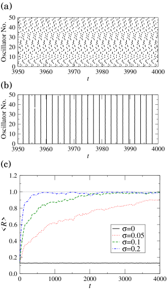
Figure 1: Synchronization of 50 Stuart-Landau oscillators driven by external impulses. (a) Zero-crossing events at $\sigma=0$ and (b) at $\sigma=0.1$. (c) Time sequence of the averaged modulus $\langle R\rangle$ of the order parameter calculated at $\sigma=0,0.05,0.1$ and $0.2$.

II Phase synchronization induced by external impulses

We first present a general model of limit-cycle oscillators driven by a common external impulsive forcing, which we will analyze in later sections. Then, before going into a general theory, we numerically demonstrate phase synchronization induced by external impulses using two typical models of limit-cycle oscillators, and briefly comment on its mechanism.

II.1 General Model

We consider an ensemble of $N$ identical limit-cycle oscillators subject to a common external impulsive forcing in the following general form:

$${\dot{\bf X}_{i}}(t)={\bf F}({\bf X}_{i})+{\bf I}(t)$$ (1)

for $i=1,\cdots,N$, where ${\bf X}_{i}(t)$ represents the internal state of the $i$-th oscillator at time $t$ and ${\bf F}$ its dynamics. We assume that Eq.(1) has a single stable limit-cycle solution ${\bf X}_{0}(t)$ in the absence of external impulsive forcing ${\bf I}(t)$, whose basin of attraction is the entire phase space except some unstable fixed points. External impulsive forcing ${\bf I}(t)$ is given by

$${\bf I}(t)=\sum_{n=1}^{\infty}{\bf e}_{n}\delta(t-t_{n}),$$ (2)

where $t_{1},t_{2},\cdots$ are occurrence times of the impulses, and ${\bf e}_{1},{\bf e}_{2},\cdots$ are random vectors representing the “direction” of the impulses. When the oscillator receives an impulse at $t=t_{n}$, its state ${\bf X}_{i}$ is suddenly kicked by a random displacement ${\bf e}_{n}$ to a new state ${\bf X}_{i}+{\bf e}_{n}$.

We assume that the direction of the impulse ${\bf e}$ is mutually independent and identically distributed. We denote its probability density by $Q({\bf e})$, which is normalized as $\int d{\bf e}Q({\bf e})=1$. We also assume the interval $T$ between two successive impulses to be independent and identically distributed. We denote its probability density function by $P(T)$, which is normalized as $\int_{0}^{\infty}dTP(T)=1$. We further assume the intervals to be sufficiently long, so that the orbit kicked away from the limit cycle by an impulse can return to the limit cycle before the next impulse. This is the necessary condition for the phase description of the oscillator, which we adopt in the following discussion. The time needed for this process of course depends on the characteristic of the oscillator and on the intensity of the impulses, which is very roughly of the order of the period of the limit cycle.

In this paper, we mainly consider impulses generated by a Poissonian process. Then Eqs.(1) and (2) describe a Poisson-driven Markov process Snyder ; Hanggi . In the Poissonian process, an impulse is generated with probability $\nu$ in an infinitesimal time interval $\Delta t$. The probability density $P(T)$ of the inter-impulse interval $T$ is given by the exponential distribution

$$P(T)=\frac{1}{\tau}\exp\left(-\frac{T}{\tau}\right),$$ (3)

where $\tau=\nu^{-1}$ determines the mean inter-impulse interval. Of course, in this Poissonian case, there exists a certain probability that the generated interval becomes shorter than the above-mentioned return time of a kicked orbit to the limit cycle. In such a case, the phase description fails to approximate the true dynamics precisely. However, when $\tau$ is sufficiently large, such probability becomes small, and the phase description would be a good approximation statistically.

The probability density of the impulse direction $Q({\bf e})$ should be chosen properly depending on the problem under consideration. For example, when we consider neural oscillators, usually only the membrane potential can be stimulated experimentally by a current injection. Therefore, the random vector ${\bf e}$ has only one non-zero element corresponding to the voltage component of ${\bf X}$, and we only need to consider one-dimensional probability density $Q(\sigma)$, where $\sigma$ is the intensity of the current impulse. In the following examples, we only treat the cases where the stimulus can take a single fixed direction and intensity ${\bf e}_{0}$, namely $Q({\bf e})=\delta({\bf e}-{\bf e}_{0})$, but we present our theory in a general form so that it is also applicable to the case where the stimulus takes various direction and intensity.

II.2 Examples

II.2.1 Stuart-Landau oscillator

Our first example is an ensemble of noisy Stuart-Landau oscillators Kuramoto driven by a common sequence of Poissonian random impulses with fixed intensity. The Stuart-Landau oscillator is the simplest limit-cycle oscillator, which is derived as a normal form of the super-critical Hopf bifurcation Kuramoto . The model is described by

$$\dot{C_{i}}(t) = (1+ic_{0})C_{i}-(1+ic_{2})|C_{i}|^{2}C_{i}+I(t)+\zeta_{i}(t)$$ (4)

for $i=1,\cdots,N$, where $C_{i}$ is the complex amplitude of the $i$-th oscillator, $c_{0}$ and $c_{2}$ are real parameters, $I(t)$ represents a sequence of external impulses, and $\zeta_{i}(t)$ is a mutually independent complex Gaussian-white noise additionally introduced to represent small external disturbances. For simplicity, we drive only the real part of $C_{i}$ by the external impulsive forcing $I(t)$, which is given by

$$I(t)=\sigma\sum_{n=1}^{\infty}\delta(t-t_{n}),$$ (5)

where the real parameter $\sigma$ represents the intensity of the impulses, $t_{n}$ the time of occurrence of the impulse, and $\delta$ the Dirac’s delta function. The impulses are generated by a Poisson process with mean inter-impulse interval $\tau$. When the oscillator receives an impulse, its real component $\mbox{Re}C_{i}$ suddenly jumps by an amount $\sigma$. It is assumed that the complex Gaussian-white noise $\zeta_{i}(t)$ has zero-mean, and whose variance is given by

$$\langle\mbox{Re}\zeta_{i}(t)\mbox{Re}\zeta_{j}(t^{\prime})\rangle = D\delta_{i,j}\delta(t-t^{\prime}),$$ (6)

$$\langle\mbox{Im}\zeta_{i}(t)\mbox{Im}\zeta_{j}(t^{\prime})\rangle = D\delta_{i,j}\delta(t-t^{\prime}),$$ (7)

$$\langle\mbox{Re}\zeta_{i}(t)\mbox{Im}\zeta_{j}(t^{\prime})\rangle = 0,$$ (8)

where $D$ determines the noise intensity. We fix the parameters at $c_{0}=2$, $c_{2}=-1$, $\tau=2$, and the noise strength at $\sqrt{D}=10^{-3}$.

We initially set the phase $\theta_{i}$ of each oscillator uniformly and randomly on $[0,1]$ (see the next section for the precise definition of the “phase”), where the zero-crossing point of $C_{i}$ from $\mbox{Im}C_{i}<0$ to $\mbox{Im}C_{i}>0$ is chosen as the origin of phase, $\theta_{i}=0$. We then evolve the oscillators under the influence of the Poissonian impulses and the weak Gaussian-white noise. Figures 1(a) and (b) plot zero-crossing events of $C_{i}$ of $N=50$ Stuart-Landau oscillators by bars (so-called raster plot) after transient for the cases $\sigma=0$ and $\sigma=0.1$. It can be seen that the oscillators synchronize in phase when $\sigma=0.1$, whereas they do not synchronize at all when $\sigma=0$. To quantify the degree of synchronization, we introduce an order parameter Kuramoto

$$R\exp(2\pi i\Theta)=\frac{1}{N}\sum_{i=1}^{N}\exp(2\pi i\theta_{i})$$ (9)

using phase $\theta_{i}$ of each oscillator. The modulus $R$ of this order parameter takes $R=1$ for complete synchronization and $R=0$ for complete desynchronization. Figure 1(c) displays temporal evolution of the modulus $\langle R\rangle$ averaged over 50 realizations from different initial conditions. It gradually increases from a small value to $1$ when $\sigma=0.05$ and $\sigma=0.1$, while it constantly takes a small value when $\sigma=0$. Thus, the uncoupled Stuart-Landau oscillators driven by a common sequence of Poissonian impulses synchronize in phase even if small external disturbances exist.

II.2.2 Hodgkin-Huxley model

Our second example is an ensemble of the Hodgkin-Huxley neural oscillators Koch driven by a common sequence of Poissonian random impulses with fixed intensity. It is given by the following set of equations Koch :

$$C_{m}\dot{V_{i}}(t) = G_{Na}m_{i}^{3}h_{i}(E_{Na}-V_{i})+G_{K}n_{i}^{4}(E_{K}-V_{i})+G_{m}(V_{rest}-V_{i})+I_{0}+I(t)+\xi_{i}(t),$$ (10)

$$\dot{m_{i}}(t) = \alpha_{m}(1-m_{i})-\beta_{m}m_{i},$$ (11)

$$\dot{h_{i}}(t) = \alpha_{h}(1-h_{i})-\beta_{h}h_{i},$$ (12)

$$\dot{n_{i}}(t) = \alpha_{n}(1-n_{i})-\beta_{n}n_{i},$$ (13)

for $i=1,\cdots,N$, where $V_{i}$ represents the membrane potential of the $i$-th neural oscillator, $m_{i}$ and $h_{i}$ the activation of its sodium channel, and $n_{i}$ the activation of the potassium channel, $I_{0}$ the constant input current, $I(t)$ the external impulsive forcing, and $\xi_{i}(t)$ the additional external disturbances. Parameters $G_{Na}$, $G_{K}$, and $G_{m}$ represent conductances of the channels, $E_{Na}$, and $E_{K}$ represent their reversal potentials, and $V_{rest}$ represents the rest voltage. $\alpha_{x}$ and $\beta_{x}$ ($x=m,h,n$) are rate constants that are given by the following equations:

$$\alpha_{m} = \frac{0.1(25-v)}{\exp(\frac{25-v}{10})-1},\;\;\;\beta_{m}=4\exp(-\frac{v}{18}),$$ (14)

$$\alpha_{h} = 0.07\exp(-\frac{v}{20}),\;\;\;\beta_{h}=\frac{1}{\exp(\frac{30-v}{10}+1)},$$ (15)

$$\alpha_{n} = \frac{0.01(10-v)}{\exp(\frac{10-v}{10})-1},\;\;\;\beta_{n}=0.125\exp(-\frac{v}{80}).$$ (16)

The parameters are fixed at the standard values presented in the textbook Koch , i.e., $G_{Na}=120$, $E_{Na}=115$, $G_{K}=36$, $E_{K}=-12$, $G_{m}=0.3$, $V_{rest}=10.613$ and $C_{m}=1$. We fix the constant input at $I_{0}=11$. When the external impulsive forcing $I(t)$ is absent, this model exhibits stable limit-cycle oscillation. The external impulsive forcing is given by

$$I(t)=\sigma\sum_{n=1}^{\infty}\delta(t-t_{n}),$$ (17)

where $\sigma$ determines its intensity. The impulses are generated by a Poissonian process with mean inter-impulse interval $\tau=100$. The external disturbance $\xi_{i}(t)$ is represented by a Gaussian-white noise of mean $0$ and variance $D$. We fix the noise strength at $\sqrt{D}=10^{-3}$ hereafter. We define the zero-crossing event (“firing event”) of this Hodgkin-Huxley neural oscillator as the moment at which the variable $V_{i}$ changes its sign from $V_{i}<0$ to $V_{i}>0$. We take this point as the origin, and define a phase along the limit cycle Winfree ; Kuramoto .

As in the previous case, we set the initial phases of the Hodgkin-Huxley oscillators randomly, and evolve them under the effect of Poissonian impulses and Gaussian-white noises. Figures 2(a),(b) show zero-crossing events of an ensemble of 50 Hodgkin-Huxley neural oscillators without or with external impulses ($\sigma=0$ or $\sigma=2$) after the initial transient. The zero-crossing event well coincides with each other when $\sigma=2$, i.e. the oscillators synchronize in phase after the initial transient. Of course, they do not synchronize at all when $\sigma=0$. Figure 2(c) shows temporal evolution of the modulus $\langle R\rangle$ of the order parameter averaged over 20 independent realizations at several values of the impulse intensity $\sigma$. When $\sigma$ takes $1$, $2$, or $4$, phase synchronization occurs and $\langle R\rangle$ gradually increases from a small value to $1$.

It is also possible to observe impulse-induced desynchronization by choosing the impulse intensity appropriately as shown in Fig. 3(a), where the zero-crossing events of 50 Hodgkin-Huxley neural oscillators are plotted. In this case, the external constant input is set at $I_{0}=9.8$, the intensity of the external impulse at $\sigma=6$, and the inter-impulse interval at $\tau=50$. The phase of each oscillator is initially set at roughly the same value, except tiny additional fluctuations of order $0.1$. To avoid spurious complete synchronization due to numerical cutoff, small external Gaussian-white noise with $\sqrt{D}=10^{-3}$ is additionally applied. The phases of the oscillators scatter occasionally, and correspondingly the order parameter drops as shown in Fig. 3(b). Thus, initial tiny phase differences among the oscillators can also be enhanced by the external impulses.

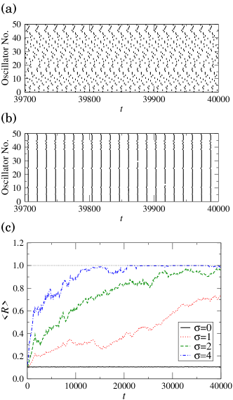
Figure 2: Synchronization of 50 Hodgkin-Huxley neural oscillators driven by external impulses. (a) Zero-crossing events at $\sigma=0$ and (b) at $\sigma=2$. (c) Time sequence of the averaged modulus $\langle R\rangle$ of the order parameter calculated at $\sigma=0,1,2$ and $4$.

Figure 3: Desynchronization of 50 Hodgkin-Huxley neural oscillators induced by external impulses. (a) Zero-crossing events. (b) Temporal sequence of the modulus $R$ of the corresponding order parameter.

II.3 Some comments on the mechanism of impulse-induced phase synchronization

The mechanism of phase synchronization induced by common external input is basically a single-oscillator problem, though we consider an ensemble of oscillators in the above examples. The origin of the phase synchronization is the local stabilization of each limit cycle in the phase direction due to the external impulses. Namely, small phase disturbances of a single oscillator shrink statistically, as we formulate in the following sections by reducing the dynamics of each oscillator to a random phase map. At the same time, it indicates the suppression of small difference in phase between any pair of oscillators. Due to random impulses, the phase of each oscillator diffuses on the limit cycle in addition to the constant rotation. Once two phases of any pair of the oscillators come close accidentally, their difference can no longer grow but shrinks statistically due to the local stability, leading to the synchrony of the entire ensemble. This mechanism has certain similarity to that of chaos synchronization induced by common random forcing Pecora ; Pikovsky ; Khoury ; Toral .

In the second example, we demonstrated that external impulses do not only lead to phase synchronization but can also cause phase desynchronization. Though we mainly focus on phase synchronization in this paper, this fact is important in understanding that fluctuation-induced phase synchronization is not a trivial phenomenon but has some subtleties.

III Reduction to a random phase map

In order to analyze the stability against phase disturbances, we first reduce the dynamics of our impulse-driven limit-cycle oscillator to a random phase map.

III.1 Random phase map

Following the standard procedure Winfree ; Kuramoto , we define a phase $\theta=\theta({\bf X}_{0})$ along the limit cycle orbit ${\bf X}_{0}(t)$ in such a way that $\theta$ increases with a constant angular velocity $\omega$. The phase $\theta$ is normalized by the period of the limit cycle, so that its range is $[0,1]$ where $0$ and $1$ represent the same phase. This definition of phase can be extended to the entire phase space except at phase-singular points, yielding a phase field $\theta({\bf X})$. It is achieved by identifying a point $P$ in the phase space with a point $Q$ right on the limit cycle in such a way that the two orbits started from $P$ and $Q$ asymptotically coincide. A set of points that have equal phase is called an isochron. The entire phase space is composed of isochrons with various phases.

In the absence of external impulses, the phase $\theta(t)=\theta({\bf X}(t))$ obeys

$$\dot{\theta}(t)=\omega$$ (18)

on the entire phase space (except at phase-singular points). When the external impulses are given, the orbit is perturbed. Let us assume that the orbit is on the limit-cycle at time $t=t_{n}-0$ , i.e. immediately before the $n$-th impulse (we say the orbit is “on” the limit cycle when it is sufficiently close to the limit cycle.) We denote its location by ${\bf X}_{0}(t_{n}-0)$ and its phase by $\theta_{n}=\theta(t_{n}-0)$. We also denote the interval between the $n$-th impulse and the next $(n+1)$-th impulse by $T_{n}=t_{n+1}-t_{n}$. When the oscillator receives an impulse ${\bf e}_{n}\delta(t-t_{n})$ at $t=t_{n}$, the orbit is kicked off the limit cycle and jumps to a new phase-space point as

$${\bf X}(t_{n}+0)={\bf X}_{0}(t_{n}-0)+{\bf e}_{n}.$$ (19)

This new phase-space point ${\bf X}(t_{n}+0)$ is on a certain isochron of the limit cycle, whose phase we denote by $\phi_{n}$ (unless it is kicked exactly onto the phase-singular point, which rarely occurs). We represent this mapping from $\theta_{n}$ to $\phi_{n}$ by

$$\phi_{n}=F(\theta_{n},{\bf e}_{n})=\theta_{n}+G(\theta_{n},{\bf e}_{n}),$$ (20)

which we call a “phase map” hereafter. In the second expression, we split $F(\theta_{n},{\bf e}_{n})$ into the trivial part $\theta_{n}$ that exists even without any impulses, and the non-trivial part $G(\theta_{n},{\bf e}_{n})$ arising from the impulse. Since $F(\theta,{\bf e})$ is a phase map, it is a periodic function on $[0,1]$. Therefore, $F(1,{\bf e})=F(0,{\bf e})$ and $G(0,{\bf e})=G(1,{\bf e})$ should hold (we should treat them in modulo $1$). As we discuss later, the above rule gives rise to an impulse-driven phase equation of the Ito-type Snyder ; Hanggi .

After the arrival of the $n$-th impulse, the oscillator evolves freely with no external impulses from $t=t_{n}+0$ to $t=t_{n+1}-0$ for an interval of $T_{n}=t_{n+1}-t_{n}$, and the phase changes from $\phi_{n}$ to $\phi_{n}+\omega T_{n}$ during this interval. If $T_{n}$ is sufficiently large, the orbit evolves from ${\bf X}(t_{n}+0)$ to a new point ${\bf X}_{0}(t_{n+1}-0)$ on the limit cycle.

Thus, corresponding to the evolution of the variable ${\bf X}_{0}(t_{n}-0)\to{\bf X}(t_{n}+0)\to{\bf X}_{0}(t_{n+1}-0)$ from $t=t_{n}-0$ to $t=t_{n+1}-0$, the phase evolves as $\theta_{n}\to\phi_{n}\to\phi_{n}+\omega T_{n}$. Hence we obtain the following evolution equation of the phase:

$$\theta_{n+1}=\omega T_{n}+F(\theta_{n},{\bf e}_{n})=\theta_{n}+\omega T_{n}+G(\theta_{n},{\bf e}_{n}).$$ (21)

Since $T_{n}$ and ${\bf e}_{n}$ are random variables whose probability density functions are given by $P(T)$ and $Q({\bf e})$ respectively, this equation describes a random map. When we consider Poissonian random impulses, the time step $n$ roughly corresponds to the real time $t$ as $n\simeq t/\tau$, because the mean inter-impulse interval is $\tau$.

If we go back to the continuous description, the dynamics of the phase $\theta$ can be written as

$$\dot{\theta}(t)=\omega+\sum_{n=1}^{\infty}G(\theta_{n},{\bf e}_{n})\delta(t-t_{n}).$$ (22)

The external impulse is now explicitly multiplicative in this equation. This impulse-driven phase equation is of Ito type Snyder ; Hanggi , namely, $G(\theta_{n},{\bf e}_{n})$ depends only on the phase $\theta_{n}$ before the $n$-th impulse, which stems from the rule we have assumed for the phase jump caused by an impulse.

III.2 Relation to the phase response function

According to the standard theory of phase reduction Winfree ; Kuramoto , when the orbit on the limit-cycle ${\bf X}_{0}$ at phase $\theta$ is kicked by a weak impulsive force ${\bf p}$ to another isochron, its new phase $\phi$ is given by a linear projection of the perturbation ${\bf p}$ on the gradient of the phase field $\theta({\bf X})$ as

$$\phi=\theta+{\bf Z}(\theta)\cdot{\bf p},$$ (23)

where

$${\bf Z}(\theta)=\nabla_{\bf X}\theta({\bf X})|_{{\bf X}_{0}(\theta)}$$ (24)

is the conventional phase response function representing the gradient of $\theta({\bf X})$ on the limit cycle orbit ${\bf X}_{0}(t)$. Comparing this equation with Eqs.(20) and (21), we obtain

$$F(\theta_{n},{\bf e}_{n})=\theta_{n}+{\bf Z}(\theta_{n})\cdot{\bf e}_{n},\;\;\;G(\theta_{n},{\bf e}_{n})={\bf Z}(\theta_{n})\cdot{\bf e}_{n},$$ (25)

so that the phase dynamics can be described by

$$\theta_{n+1}=\theta_{n}+\omega T_{n}+{\bf Z}(\theta_{n})\cdot{\bf e}_{n}.$$ (26)

Thus, for sufficiently small ${\bf e}_{n}$, the phase map can simply be represented using the inner product of the conventional phase response function ${\bf Z}(\theta)$ and the direction of the impulse ${\bf e}_{n}$.

III.3 Generalized Frobenius-Perron equation

Temporal evolution of the probability density function (PDF) $\rho(\theta,n)$ of the phase $\theta$ at time step $n$ is described by a generalized Frobenius-Perron equation Lasota , which is convoluted with a transition kernel $W(\theta)$ that represents random shifting on the limit cycle for a random duration $T$ drawn from $P(T)$, and is also averaged by the probability density $Q({\bf e})$ of impulse directions ${\bf e}$,

$$\rho(\theta,n+1)=\int_{0}^{1}d\phi W(\theta-\phi)\int d{\bf e}Q({\bf e})\int_{0}^{1}d\psi\delta(\phi-F(\psi,{\bf e}))\rho(\psi,n),$$ (27)

where the argument $\theta-\phi$ of $W(\theta-\phi)$ should be interpreted in modulo $1$. In deriving this equation, we utilized the fact that $\theta_{n}$, ${\bf e}_{n}$, and $T_{n}$ are mutually independent ($\theta_{n}$ depends only on ${\bf e}_{1},\cdots,{\bf e}_{n-1}$ and $T_{1},\cdots,T_{n-1}$) Lasota .

For Poissonian impulses, the explicit form of the transition kernel $W(\theta)$ can be calculated from Eq.(3) by taking into account the periodicity in $\theta$ and the Jacobian of the transformation, which is given by

$$W(\theta)=\frac{1}{\omega}\sum_{j=0}^{\infty}P(\frac{\theta+j}{\omega})=\frac{e^{-\theta/(\omega\tau)}}{\omega\tau\left(1-e^{-1/\omega\tau}\right)}=\frac{A}{1-e^{-A}}e^{-A\phi}\;\;\;(0\leq\theta\leq 1),$$ (28)

where we defined $A=1/\omega\tau$. Of course, it is normalized as $\int_{0}^{1}d\theta W(\theta)=1$.

Sufficiently after the initial transient, the PDF $\rho(\theta,n)$ is expected to reach a stationary state $\rho(\theta)$, but it is generally difficult to calculate this stationary PDF analytically even if the map $F(\theta,{\bf e})$ has a simple functional form. In the following, we first analyze the limit of large inter-impulse interval $\tau$ where the stationary PDF becomes uniform, and then analyze the deviation of the stationary PDF from the uniform density perturbatively for small impulse intensity.

III.4 Examples of phase maps

III.4.1 Stuart-Landau oscillator

Figure 4(a) plots numerically calculated phase maps $F(\theta,\sigma)$ of the Stuart-Landau oscillator at several values of the impulse intensity $\sigma$. As $|\sigma|$ becomes larger, the phase map deforms from the trivial identity map noticeably, and finally becomes non-monotonic when $\sigma\simeq\pm 0.8$. Figure 4(b) displays the phase response normalized by the impulse intensity $\left[F(\theta,\sigma)-\theta\right]/\sigma=G(\theta,\sigma)/\sigma$ at several values of $\sigma$. If $\sigma$ is sufficiently small, Eq.(25) should hold, and the different curves corresponding to different values of $\sigma$ should collapse. The limiting curve at $\sigma\to 0$ gives the real component of the phase response function ${\bf Z}(\theta)$. It can be analytically calculated for the Stuart-Landau oscillator as $Z_{\mbox{Re}}(\theta)=\sin(2\pi\theta+3\pi/4)/3\sqrt{2}$ Kuramoto , which is also shown in the figure.

III.4.2 Hodgkin-Huxley model

Figure 5(a) shows numerically calculated phase maps $F(\theta,\sigma)$ of a Hodgkin-Huxley neural oscillator at several values of the impulse intensity $\sigma$. As $|\sigma|$ becomes larger, the phase map deforms from the trivial identity map and finally becomes non-monotonic at $\sigma\simeq\pm 5$. Figure 5(b) shows normalized phase response $\left[F(\theta,\sigma)-\theta\right]/\sigma=G(\theta,\sigma)/\sigma$ at several values of $\sigma$. It can be seen that the curves actually collapse at small $\sigma$, and deviates at larger $\sigma$. The liming curve at $\sigma\to 0$ gives the $V$-component of the phase response function $Z_{V}(\theta)$. The curve corresponding to $\sigma=0.1$ in Fig. 5(b) gives an approximation to the phase response function.

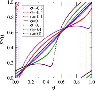
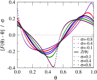
Figure 4: (a)Phase maps $F(\theta,\sigma)$ of the Stuart-Landau oscillator at several values of the impulse intensity $\sigma$. (b) Normalized phase response $\left[F(\theta)-\theta\right]/\sigma$ at several values of the impulse intensity $\sigma$. Theoretical phase response function $Z_{\mbox{Re}}(\theta)=\sin(2\pi\theta+3\pi/4)/3\sqrt{2}$ that corresponds to the limit of $\sigma\to 0$ is also shown.

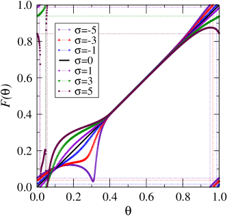
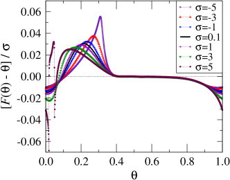
Figure 5: (a) Phase map $F(\theta,\sigma)$ of the Hodgkin-Huxley neural oscillator at several values of the impulse intensity $\sigma$. (b) Normalized phase response $\left[F(\theta)-\theta\right]/\sigma$ at several values of the impulse intensity $\sigma$. The curve corresponding to $\sigma=0.1$ gives an approximation to the phase response function $Z_{V}(\theta)$ of the Hodgkin-Huxley neural oscillator.

IV Stability in the phase direction

Synchrony of uncoupled oscillators induced by external impulses is the result of statistical stabilization of each oscillator against phase disturbances. Such stability is characterized by the Lyapunov exponent of the random phase map Eq. (21).

IV.1 Lyapunov exponent

Let us consider the temporal evolution of a small deviation $\Delta\theta_{n}$ from the original orbit $\theta_{n}$. The linearized evolution equation of this small deviation is given by

$$\Delta\theta_{n+1}=F^{\prime}(\theta_{n},{\bf e}_{n})\Delta\theta_{n},$$ (29)

where $F^{\prime}(\theta_{n},{\bf e})=\left(dF(\theta,{\bf e})/d\theta\right)_{\theta=\theta_{n}}$. At large time step $n$, $\Delta\theta_{n}$ expands as

$$\left|\frac{\Delta\theta_{n}}{\Delta\theta_{0}}\right| = \prod_{m=0}^{n-1}|F^{\prime}(\theta_{m},{\bf e}_{m})|$$ (30)

$$= \exp\left[\sum_{m=0}^{n-1}\log|F^{\prime}(\theta_{m},{\bf e}_{m})|\right]$$ (31)

$$\simeq \exp\left(\lambda n\right),$$ (33)

where we introduced the Lyapunov exponent $\lambda$ of the map $F(\theta,{\bf e})$ averaged over the PDFs $Q({\bf e})$ and $\rho(\theta)$,

$$\lambda=\langle\langle\log|F^{\prime}(\theta,{\bf e})|\rangle\rangle_{\theta,{\bf e}}=\int_{0}^{1}d\theta\rho(\theta)\int d{\bf e}Q({\bf e})\log|F^{\prime}(\theta,{\bf e})|.$$ (34)

If $\lambda$ is negative, $\Delta\theta_{n}$ shrinks on average, so that the deviation from the original orbit is suppressed, whereas if $\lambda$ is positive, small external disturbances will be enhanced. Thus, the value of $\lambda$ gives a (local) condition for the phase synchronization.

IV.2 Limit of large inter-impulse intervals

As we mentioned previously, it is difficult to obtain the stationary PDF $\rho(\theta)$ analytically. However, when the inter-impulse interval $\tau$ is sufficiently large, it can be approximated by a uniform density. In the limit of large $\tau$, the transition probability tends to be uniform, i.e. $W(\theta)\to 1$, which can easily be confirmed from Eq. (28) in the Poissonian case. Correspondingly, the stationary phase PDF $\rho(\theta)$ approaches a uniform density in the large $\tau$ limit:

$$\rho(\theta)\to 1.$$ (35)

In this limit, we can obtain a sufficient condition of phase synchronization for general limit-cycle oscillators: when the phase map $F(\theta,{\bf e})$ is a monotonically increasing function of $\theta$, the Lyapunov exponent $\lambda$ is always non-positive, namely, when $F^{\prime}(\theta,{\bf e})=1+G^{\prime}(\theta,{\bf e})>0$ is satisfied. We can then bound $\lambda$ from above as

$$\lambda = \int_{0}^{1}d\theta\rho(\theta)\int d{\bf e}Q({\bf e})\log F^{\prime}(\theta,{\bf e})$$ (36)

$$\leq \int_{0}^{1}d\theta\rho(\theta)\log\left[\int d{\bf e}Q({\bf e})F^{\prime}(\theta,{\bf e})\right]$$ (38)

$$= \int_{0}^{1}d\theta\rho(\theta)\log\left[1+\int d{\bf e}Q({\bf e})G^{\prime}(\theta,{\bf e})\right]$$ (40)

$$\leq \int_{0}^{1}d\theta\rho(\theta)\int d{\bf e}Q({\bf e})G^{\prime}(\theta,{\bf e}).$$ (42)

In the above transformation, we utilized Jensen’s inequality $\int d{\bf e}Q({\bf e})\log[g({\bf e})]\leq\log[\int d{\bf e}Q({\bf e})g({\bf e})]$ that holds for a concave function $\log[\cdots]$, the normalized probability density $Q({\bf e})$, and a positive scalar function $g({\bf e})$. The second inequality follows from $\log(1+x)\leq x$. By using the facts that $\rho(\theta)\equiv 1$ and $G(0,{\bf e})=G(1,{\bf e})$, the upper bound of $\lambda$ can be calculated as

$$\int_{0}^{1}d\theta\rho(\theta)\int d{\bf e}Q({\bf e})G^{\prime}(\theta,{\bf e})$$ (43)

$$= \int d{\bf e}Q({\bf e})\int_{0}^{1}d\theta G^{\prime}(\theta,{\bf e})$$ (45)

$$= \int d{\bf e}Q({\bf e})\left[G(1,{\bf e})-G(0,{\bf e})\right]=0.$$ (47)

Thus, for monotonically increasing $F(\theta,{\bf e})$, the Lyapunov exponent $\lambda$ is always non-positive. The equality $\lambda=0$ holds only when $F(\theta,{\bf e})$ is a trivial identity map for all ${\bf e}$, i.e. $F(\theta,{\bf e})=\theta$, which follows from the equality condition of Jensen’s inequality. Therefore, small deviations from the original orbit always shrink by applying random external impulses with large inter-impulse intervals, when the phase map $F(\theta,{\bf e})$ is monotonic.

As we mentioned previously, when ${\bf e}$ is small, $G(\theta,{\bf e})$ can be represented using the phase response function ${\bf Z}(\theta)$ as $G(\theta,{\bf e})\simeq{\bf Z}(\theta)\cdot{\bf e}$. Since $F(\theta,{\bf e})=\theta+G(\theta,{\bf e})$, $F(\theta,{\bf e})$ is monotonically increasing with respect to $\theta$ for sufficiently small ${\bf e}$. Therefore, when the intensity of external impulses is small and the mean interval between impulses is large, $\lambda$ always becomes negative.

IV.3 Examples

IV.3.1 Stuart-Landau oscillator

As can be seen from Fig. 4(a), the phase map $F(\theta,\sigma)$ of the Stuart-Landau oscillator is monotonic as long as $|\sigma|$ is small. Therefore, the Stuart-Landau oscillator exhibits phase synchronization induced by external impulses at such values of $|\sigma|$ for sufficiently large inter-impulse intervals, as we demonstrated previously.

IV.3.2 Hodgkin-Huxley model

Similarly, as shown in Fig. 5(a), numerically calculated phase maps $F(\theta,\sigma)$ of the Hodgkin-Huxley neural oscillator are monotonic when $|\sigma|$ is not so large. Therefore, the Hodgkin-Huxley neural oscillators also exhibit impulse-induced phase synchronization for such values of $|\sigma|$. When $|\sigma|$ becomes large, the phase map can become quite complex, which can lead to the impulse-induced phase desynchronization mentioned previously.

V Effect of non-uniform phase distribution

In the previous section, we discussed the limiting case of large inter-impulse intervals, where the stationary PDF of the phase becomes uniform. If the mean inter-impulse interval is not so large, the stationary PDF would generally become non-uniform. In this section, we first develop a perturbation theory to approximate the non-uniform PDF for weak external impulses. We then discuss the correction to the upper bound of the Lyapunov exponent caused by the non-uniformity of the PDF. In the following discussion, we assume that the intensity of external impulses is sufficiently small, and that the phase map $F(\theta,{\bf e})$ is a strictly monotonically increasing function of $\theta$, i.e. $F^{\prime}(\theta,{\bf e})>0$.

V.1 Perturbative solution to the generalized Frobenius-Perron equation

As a first step, we calculate the deviation of the stationary PDF from the uniform density perturbatively for small external impulses (up to the second order). Our starting point is the generalized Frobenius-Perron equation for the stationary PDF $\rho(\theta)$,

$$\rho(\theta)=\int_{0}^{1}d\phi W(\theta-\phi)\int d{\bf e}Q({\bf e})\int_{0}^{1}d\psi\delta(\phi-F(\psi,{\bf e}))\rho(\psi).$$ (48)

We assume that the deviation of $F(\theta,{\bf e})$ from the identity map $F(\theta,{\bf e})=\theta$ is small,

$$F(\theta,{\bf e})=\theta+\epsilon G(\theta,{\bf e}),$$ (49)

where we introduced a small parameter $\epsilon$ in order to control the magnitude of the perturbation. By using a well-known formula for the $\delta$-function, Eq.(48) can be rewritten as

$$\rho(\theta)=\int_{0}^{1}d\phi W(\theta-\phi)\int d{\bf e}Q({\bf e})\frac{\rho(\psi^{*}(\phi,{\bf e}))}{|F^{\prime}(\psi^{*}(\phi,{\bf e}),{\bf e})|},$$ (50)

where $\psi^{*}(\phi,{\bf e})$ is a solution to $F(\psi,{\bf e})=\phi$. We here used the fact that there exists only one solution, because $F(\psi,{\bf e})$ is a monotonically increasing function of $\psi$ (we do not consider the trivial case of $F(\psi,{\bf e})\equiv\psi$, where $\rho(\theta)$ always becomes uniform).

We first calculate the solution $\psi^{*}(\phi,{\bf e})$ to $F(\psi,{\bf e})=\phi$ as a power series in $\epsilon$. We assume that the solution can be expanded in terms of $\epsilon$ around the trivial solution $\psi^{*}(\phi,{\bf e})=\phi$ at $\epsilon=0$ as

$$\psi^{*}(\phi,{\bf e})=\phi+\epsilon\psi_{1}^{*}(\phi,{\bf e})+\epsilon^{2}\psi_{2}^{*}(\phi,{\bf e})+O(\epsilon^{3}).$$ (51)

By inserting this expression to $F(\psi^{*}(\phi,{\bf e}),{\bf e})=\phi$, we obtain

$$\phi = \phi\;\;\;\mbox{at}\;\;O(\epsilon^{0}),$$ (52)

$$\psi_{1}^{*}(\phi,{\bf e})+G(\phi,{\bf e}) = 0\;\;\;\mbox{at}\;\;O(\epsilon^{1}),$$ (53)

$$\psi_{2}^{*}(\phi,{\bf e})+G^{\prime}(\phi,{\bf e})\psi_{1}^{*}(\phi,{\bf e}) = 0\;\;\;\mbox{at}\;\;O(\epsilon^{2}),$$ (54)

$$\cdots$$ . (55)

Thus, to the second order in $\epsilon$, the solution $\psi^{*}(\phi,{\bf e})$ is approximated by

$$\psi^{*}(\phi,{\bf e})=\phi-\epsilon G(\phi,{\bf e})+\epsilon^{2}G^{\prime}(\phi,{\bf e})G(\phi,{\bf e})+O(\epsilon^{3}).$$ (56)

Since $F^{\prime}(\theta,{\bf e})=1+\epsilon G^{\prime}(\theta,{\bf e})$, it can be expanded as

$$F^{\prime}(\psi^{*}(\phi,{\bf e}),{\bf e})=1+\epsilon G^{\prime}(\phi,{\bf e})-\epsilon^{2}G^{\prime\prime}(\phi,{\bf e})G(\phi,{\bf e})+O(\epsilon^{3}).$$ (57)

We also expand the stationary PDF $\rho(\theta)$ in a power series of $\epsilon$ as

$$\rho(\theta)=1+\epsilon\rho_{1}(\theta)+\epsilon^{2}\rho_{2}(\theta)+O(\epsilon^{3}).$$ (58)

Since $\rho(\theta)$ is normalized to $1$, $\int_{0}^{1}d\theta\rho_{1}(\theta)=\int_{0}^{1}d\theta\rho_{2}(\theta)=0$ should hold. Inserting the above expansions into Eq.(50), we obtain

$$1+\epsilon\rho_{1}(\theta)+\epsilon^{2}\rho_{2}(\theta)+O(\epsilon^{3})$$ (59)

$$= \int_{0}^{1}d\phi W(\theta-\phi)\int d{\bf e}Q({\bf e})\frac{1+\epsilon\rho_{1}(\phi)+\epsilon^{2}\left\{\rho_{2}(\phi)-\rho_{1}^{\prime}(\phi)G(\phi,{\bf e})\right\}+O(\epsilon^{3})}{1+\epsilon G^{\prime}(\phi,{\bf e})-\epsilon^{2}G^{\prime\prime}(\phi,{\bf e})G(\phi,{\bf e})+O(\epsilon^{3})}$$ (61)

$$= \int_{0}^{1}d\phi W(\theta-\phi)\int d{\bf e}Q({\bf e})\left[1+\epsilon\left\{\rho_{1}(\phi)-G^{\prime}(\phi,{\bf e})\right\}+\epsilon^{2}\left\{\rho_{2}(\phi)-H(\phi,{\bf e})\right\}+O(\epsilon^{3})\right]$$ (63)

where we utilized the fact that $F^{\prime}(\psi^{*}(\phi,{\bf e}),{\bf e})>0$, and defined

$$H(\phi,{\bf e})=\rho_{1}(\phi)G(\phi,{\bf e})-G^{\prime}(\phi,{\bf e})G(\phi,{\bf e}).$$ (64)

Thus, the first order correction $\rho_{1}(\theta)$ to the uniform stationary PDF $\rho_{0}(\theta)\equiv 1$ satisfies

$$\rho_{1}(\theta) = \int_{0}^{1}d\phi W(\theta-\phi)\int d{\bf e}Q({\bf e})\left\{\rho_{1}(\phi)-G^{\prime}(\phi,{\bf e})\right\}$$ (65)

$$= \int_{0}^{1}d\phi W(\theta-\phi)\left\{\rho_{1}(\phi)-\langle G^{\prime}\rangle_{\bf e}(\phi)\right\},$$ (67)

and the second order correction $\rho_{2}(\theta)$ satisfies

$$\rho_{2}(\theta) = \int_{0}^{1}d\phi W(\theta-\phi)\int d{\bf e}Q({\bf e})\left\{\rho_{2}(\phi)-H^{\prime}(\phi,{\bf e})\right\}$$ (68)

$$= \int_{0}^{1}d\phi W(\theta-\phi)\left\{\rho_{2}(\phi)-\langle H^{\prime}\rangle_{\bf e}(\phi)\right\}.$$ (70)

Here and hereafter, for notational simplicity, we define an averaged function $\langle f\rangle_{\bf e}(\theta)$ of a function $f(\theta,{\bf e})$ over $Q({\bf e})$ as

$$\langle f\rangle_{\bf e}(\theta)=\int d{\bf e}Q({\bf e})f(\theta,{\bf e}),$$ (71)

such as $\langle G^{\prime}\rangle_{\bf e}(\phi)=\int d{\bf e}Q({\bf e})G^{\prime}(\phi,{\bf e})$ and $\langle H^{\prime}\rangle_{\bf e}(\phi)=\int d{\bf e}Q({\bf e})H^{\prime}(\phi,{\bf e})$. We also define the Fourier transform between a function $f(\theta)$ and its coefficient $\tilde{f}(k)$ by

$$f(\theta)=\sum_{k=-\infty}^{\infty}e^{2\pi ik\theta}\tilde{f}(k),\;\;\;\tilde{f}(k)=\int_{0}^{1}d\theta e^{-2\pi ik\theta}f(\theta).$$ (72)

For example, the Fourier coefficients of $\rho_{1}(\theta)$ and $G^{\prime}(\theta,{\bf e})$ are denoted as $\tilde{\rho_{1}}(k)$ and $\tilde{G^{\prime}}(k,{\bf e})$, respectively. The averaged Fourier coefficient $\langle\tilde{f}\rangle_{\bf e}(k)$ of $\tilde{f}(k,{\bf e})$ over $Q({\bf e})$ is similarly defined as

$$\langle\tilde{f}\rangle_{\bf e}(k)=\int d{\bf e}Q({\bf e})\tilde{f}(k,{\bf e}),$$ (73)

such as $\langle\tilde{G^{\prime}}\rangle_{\bf e}(m)=\int d{\bf e}Q({\bf e})\tilde{G^{\prime}}(m,{\bf e})$ and $\langle\tilde{H^{\prime}}\rangle_{\bf e}(m)=\int d{\bf e}Q({\bf e})\tilde{H^{\prime}}(m,{\bf e})$.

Equations (67) and (70) can be solved for $\rho_{1}(\theta)$ and $\rho_{2}(\theta)$ through the Fourier transform, which yields

$$\tilde{\rho_{1}}(m) = \int d{\bf e}Q({\bf e})\tilde{W}(m)\left\{\tilde{\rho_{1}}(m)-\tilde{G^{\prime}}(m,{\bf e})\right\}=\tilde{W}(m)\left\{\tilde{\rho_{1}}(m)-\langle\tilde{G^{\prime}}\rangle_{\bf e}(m)\right\},$$ (74)

and

$$\tilde{\rho_{2}}(m) = \int d{\bf e}Q({\bf e})\tilde{W}(m)\left\{\tilde{\rho_{2}}(m)-\tilde{H^{\prime}}(m,{\bf e})\right\}=\tilde{W}(m)\left\{\tilde{\rho_{2}}(m)-\langle\tilde{H^{\prime}}\rangle_{\bf e}(m)\right\}.$$ (75)

It can easily be shown that the equations at $m=0$ give trivial relations, which should be neglected. We thus obtain

$$\tilde{\rho_{1}}(m)=\frac{\tilde{W}(m)}{\tilde{W}(m)-1}\langle\tilde{G^{\prime}}\rangle_{\bf e}(m),\;\;\;\tilde{\rho_{2}}(m)=\frac{\tilde{W}(m)}{\tilde{W}(m)-1}\langle\tilde{H^{\prime}}\rangle_{\bf e}(m)$$ (76)

for $m\neq 0$, and the corrections $\rho_{1}(\theta)$ and $\rho_{2}(\theta)$ to the uniform density can be obtained as

$$\rho_{1}(\theta)=\sum_{m\neq 0}\frac{\tilde{W}(m)}{\tilde{W}(m)-1}\langle\tilde{G^{\prime}}\rangle_{\bf e}(m)e^{2\pi im\theta},\;\;\;\rho_{2}(\theta)=\sum_{m\neq 0}\frac{\tilde{W}(m)}{\tilde{W}(m)-1}\langle\tilde{H^{\prime}}\rangle_{\bf e}(m)e^{2\pi im\theta}.$$ (77)

For the Poissonian impulses, the transition probability $W(\theta)$ is given by Eq. (28), and its Fourier coefficient $\tilde{W}(m)$ is given by

$$\tilde{W}(m)=\int_{0}^{1}d\theta W(\theta)e^{-2\pi im\theta}=\frac{A}{A+2\pi im}$$ (78)

for integer $m$. Therefore, the coefficient in Eq.(77) is calculated as $\tilde{W}(m)/[\tilde{W}(m)-1]=-A/(2\pi im)$. Using this, we can calculate the first order correction to the phase PDF as

$$\rho_{1}(\theta) = \sum_{m\neq 0}\frac{-A}{2\pi im}\langle\tilde{G^{\prime}}\rangle_{\bf e}(m)\;e^{2\pi im\theta}=-A\sum_{m\neq 0}\langle\tilde{G}\rangle_{\bf e}(m)\;e^{2\pi im\theta}$$ (79)

$$= -A\left[\langle G\rangle_{\bf e}(\theta)-G_{0}\right],$$ (81)

where we defined $G_{0}=\langle\tilde{G}\rangle_{\bf e}(0)=\int_{0}^{1}d\theta\langle G\rangle_{\bf e}(\theta)$, and utilized the relation $\langle\tilde{G^{\prime}}\rangle_{\bf e}(m)=(2\pi im)\langle\tilde{G}\rangle_{\bf e}(m)$. Similarly, the second order correction to the PDF can be calculated as

$$\rho_{2}(\theta) = \sum_{m\neq 0}\frac{-A}{2\pi im}\langle\tilde{H^{\prime}}\rangle_{\bf e}(m)\;e^{2\pi im\theta}=-A\sum_{m\neq 0}\langle\tilde{H}\rangle_{\bf e}(m)\;e^{2\pi im\theta}$$ (82)

$$= -A\left[\langle H\rangle_{\bf e}(\theta)-\langle\tilde{H}\rangle_{\bf e}(0)\right],$$ (84)

$$= -A\left[\langle\rho_{1}(\phi)G(\phi,{\bf e})\rangle_{\bf e}-\langle G^{\prime}G\rangle_{\bf e}(\theta)\right]+const.$$ (86)

$$= A^{2}\left[\langle G\rangle_{\bf e}(\theta)\right]^{2}-A^{2}G_{0}\cdot\langle G\rangle_{\bf e}(\theta)+A\langle G^{\prime}G\rangle_{\bf e}(\theta)+const.,$$ (88)

where we defined $\langle G^{\prime}G\rangle_{\bf e}(\theta)=\langle G^{\prime}(\theta,{\bf e})G(\theta,{\bf e})\rangle_{\bf e}$. The constant can be determined from the condition $\int_{0}^{1}d\theta\rho_{2}(\theta)=0$.

Thus, in the Poissonian case, the averaged phase map $\langle G\rangle_{\bf e}(\theta)$ directly appears at the first order perturbation to the PDF, $\rho_{1}(\theta)$. Since $A=1/\omega\tau$, the amplitude of the first order perturbation scales as $\epsilon/\omega\tau$, namely, the ratio of the impulse intensity to the non-dimensional time scale determined by the period of the limit cycle and the inter-impulse intervals. The second order perturbation $\rho_{2}(\theta)$ gives lowest-order nonlinear contributions from the phase map.

V.2 Upper bound of the Lyapunov exponent

The Lyapunov exponent $\lambda$ is bounded from above as

$$\lambda = \langle\langle\log F^{\prime}(\theta,{\bf e})\rangle\rangle_{\theta,{\bf e}}$$ (89)

$$= \int_{0}^{1}d\theta\rho(\theta)\int d{\bf e}Q({\bf e})\log F^{\prime}(\theta,{\bf e})$$ (91)

$$\leq \int_{0}^{1}d\theta\rho(\theta)\log\left\{\int d{\bf e}Q({\bf e})F^{\prime}(\theta,{\bf e})\right\}$$ (93)

$$= \int_{0}^{1}d\theta\rho(\theta)\log\left\{1+\int d{\bf e}Q({\bf e})\epsilon G^{\prime}(\theta,{\bf e})\right\}$$ (95)

$$\leq \int_{0}^{1}d\theta\rho(\theta)\int d{\bf e}Q({\bf e})\left\{\epsilon G^{\prime}(\theta,{\bf e})\right\}.$$ (97)

Now, using Eq. (58), correction to the upper bound of the Lyapunov exponent can be expanded as

$$\int_{0}^{1}d\theta\rho(\theta)\int d{\bf e}Q({\bf e})\left\{\epsilon G^{\prime}(\theta,{\bf e})\right\}$$ (98)

$$= \int_{0}^{1}d\theta\left\{1+\epsilon\rho_{1}(\theta)+\epsilon\rho_{2}(\theta)+O(\epsilon^{3})\right\}\int d{\bf e}Q({\bf e})\left\{\epsilon G^{\prime}(\theta,{\bf e})\right\}$$ (100)

$$= \epsilon\int_{0}^{1}d\theta\langle G^{\prime}\rangle_{\bf e}(\theta)+\epsilon^{2}\int_{0}^{1}d\theta\rho_{1}(\theta)\langle G^{\prime}\rangle_{\bf e}(\theta)+\epsilon^{3}\int_{0}^{1}d\theta\rho_{2}(\theta)\langle G^{\prime}\rangle_{\bf e}(\theta)+O(\epsilon^{4}).$$ (102)

The first term corresponds to the (zero-th order) contribution from the uniform component of the phase PDF, which vanishes (similarly to the uniform case) irrespective of the functional form of the transition kernel $W(\theta)$,

$$\int_{0}^{1}d\theta\langle G^{\prime}\rangle_{\bf e}(\theta)=\langle G^{\prime}\rangle_{\bf e}(1)-\langle G^{\prime}\rangle_{\bf e}(0)=0.$$ (103)

For the Poissonian impulses, the first order correction to the upper bound of $\lambda$ can be calculated using Eq.(81) as

$$\int_{0}^{1}d\theta\rho_{1}(\theta)\langle G^{\prime}\rangle_{\bf e}(\theta)$$ (104)

$$= -A\int_{0}^{1}d\theta\langle G\rangle_{\bf e}\langle G^{\prime}\rangle_{\bf e}(\theta)+AG_{0}\int_{0}^{1}d\theta\langle G^{\prime}\rangle_{\bf e}(\theta)$$ (106)

$$= -A\left[\frac{\left\{\langle G\rangle_{\bf e}(\theta)\right\}^{2}}{2}\right]_{0}^{1}+AG_{0}\left[\langle G\rangle_{\bf e}(\theta)\right]_{0}^{1}$$ (108)

$$= 0.$$ (110)

Thus, the upper bound of the Lyapunov exponent $\lambda$ is still zero even if the first order correction to the uniform PDF is incorporated. The second order correction to the upper bound can similarly be calculated using Eq.(88) as

$$\int_{0}^{1}d\theta\rho_{2}(\theta)\langle G^{\prime}\rangle_{\bf e}(\theta)$$ (111)

$$= A^{2}\int_{0}^{1}d\theta\left\{\langle G\rangle_{\bf e}(\theta)\right\}^{2}\langle G^{\prime}\rangle_{\bf e}(\theta)-A^{2}G_{0}\int_{0}^{1}d\theta\left\{\langle G\rangle_{\bf e}(\theta)\right\}\langle G^{\prime}\rangle_{\bf e}(\theta)$$ (115)

$$+A\int_{0}^{1}d\theta\langle G^{\prime}G\rangle_{\bf e}(\theta)\langle G^{\prime}\rangle_{\bf e}(\theta)+const.\int_{0}^{1}d\theta\langle G^{\prime}\rangle_{\bf e}(\theta)$$

$$= \frac{A^{2}}{3}\left[\left\{\langle G^{\prime}\rangle_{\bf e}(\theta)\right\}^{3}\right]_{0}^{1}-\frac{A^{2}G_{0}}{2}\left[\left\{\langle G^{\prime}\rangle_{\bf e}(\theta)\right\}^{2}\right]_{0}^{1}$$ (119)

$$+const.\left[\left\{\langle G^{\prime}\rangle_{\bf e}(\theta)\right\}^{2}\right]_{0}^{1}+A\int_{0}^{1}d\theta\langle G^{\prime}G\rangle_{\bf e}(\theta)\langle G^{\prime}\rangle_{\bf e}(\theta)$$

$$= A\int_{0}^{1}d\theta\langle G^{\prime}G\rangle_{\bf e}(\theta)\langle G^{\prime}\rangle_{\bf e}(\theta).$$ (121)

Thus, only the term containing $\langle G^{\prime}G\rangle_{\bf e}(\theta)$ in $\rho_{2}(\theta)$ gives non-vanishing contribution. Its sign cannot be determined at this point unless the explicit functional form of $G(\theta,{\bf e})$ is given. This term could make the upper bound of the Lyapunov exponent slightly different from zero, but its effect is only of the order of $\epsilon^{3}$.

Summarizing, the first order correction to the upper bound of the Lyapunov exponent $\lambda$ by the non-uniformity of the phase PDF is generally $O(\epsilon^{2})$, but for the Poissonian impulses, it vanishes. Thus, the upper bound of $\lambda$ is still zero up to the first order approximation. The next order correction is only $O(\epsilon^{3})$, which is quite small when $\epsilon$ is small. Therefore, the impulse-induced phase synchronization will, in most cases, persist for weak Poissonian impulses even if the phase PDF becomes slightly non-uniform for small $\epsilon$.

V.3 Examples of Lyapunov exponents

V.3.1 Stuart-Landau oscillator

Stationary phase PDFs $\rho(\theta)$ of the Stuart-Landau oscillator driven by external impulses at $\sigma=0.1$ and $\tau=2$ are shown in Figure 6. The curves are obtained by (i) a direct simulation of the original model Eq.(4) without Gaussian-white noise, (ii) a direct simulation of the reduced phase model Eq.(22), (iii) a numerical calculation of the stationary solution of the corresponding Frobenius-Perron equation Eq.(48), and (iv) the perturbation theory up to the second order, respectively. All curves agree well, which confirms the validity of our approximation at least for small impulse intensity. In this case, the first order perturbation already gives a nice fit to the actual PDF, and the second order perturbation gives only a tiny correction.

Figure 7 plots the Lyapunov exponent $\lambda$ as a function of $\sigma$ at $\tau=2$, which is obtained by (i) directly using the original model Eq.(4) without Gaussian-white noise, (ii) directly using the reduced phase model Eq.(22), (iii) a calculation using numerical phase maps and uniform phase PDF, and (iv) a calculation using numerical phase maps and the approximated phase PDF. Reflecting the symmetry of the limit cycle, the graph of $\lambda$ is also symmetrical with respect to $\sigma=0$. Since the phase map is always monotonically increasing in this range of $\sigma$, the Lyapunov exponent $\lambda$ calculated assuming uniform phase PDF (iii) is always non-positive and only becomes $0$ when $\sigma=0$. The Lyapunov exponent $\lambda$ calculated using approximate phase PDF (iv) is also always non-positive. Since the correction to the uniform PDF is small, the difference between (iii) and (iv) is also small. Both curves agree well with the actual Lyapunov exponent obtained by (i) and (ii).

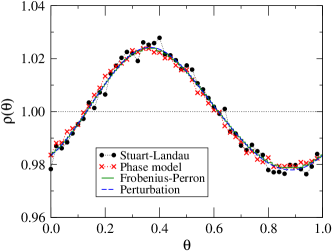
Figure 6: Stationary phase PDFs of the Stuart-Landau oscillator driven by external impulses obtained by (i) a direct simulation of the original model, (ii) a direct simulation of the corresponding phase model, (iii) numerically solving the corresponding Frobenius-Perron equation, and (iv) the perturbation theory.

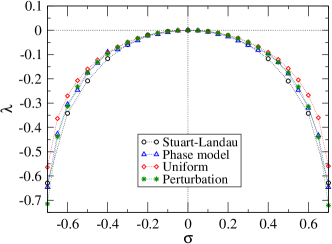
Figure 7: Dependence of the Lyapunov exponent $\lambda$ on the impulse intensity $\sigma$ obtained by (i) directly using the original model Eq.(4) without Gaussian-white noise, (ii) directly using the reduced phase model Eq.(22), (iii) a calculation using numerical phase maps assuming uniform phase PDF, and (iv) a calculation using numerical phase maps and the approximated phase PDF.

V.3.2 Hodgkin-Huxley model

Similarly, stationary PDFs of the Hodgkin-Huxley neural oscillator driven by external impulses at $\sigma=2$ and $\tau=100$ are shown in Figure 8. As previous, the curves represent the results obtained by (i) a direct simulation of the original model, (ii) a direct simulation of the reduced phase model, (iii) a numerical solution of the Frobenius-Perron equation, and (iv) the perturbation theory. Of course, the results of (ii) and (iii) give a nice fit to the actual phase PDF obtained by (i). The result of perturbation theory (iv) also gives a reasonable fit to the actual phase PDF. As in the previous case, the first order perturbation gives a good fit to the actual PDF, and the second order perturbation gives only a tiny correction.

Figure 9 plots the Lyapunov exponent $\lambda$ as a function of $\sigma$ at $\tau=100$, which is obtained by (i) directly simulating the original model without external disturbances, (ii) directly simulating the reduced phase model, (iii) calculation using numerical phase maps assuming uniform phase PDF, and (iv) calculation using numerical phase maps and the phase PDF approximated up to the second order perturbation. Since the phase map is always monotonically increasing in this range of $\sigma$, the Lyapunov exponent $\lambda$ calculated assuming uniform phase PDF (iii) is always non-positive and only becomes $0$ when $\sigma=0$. The Lyapunov exponent $\lambda$ calculated using approximate phase PDF (iv) is also always non-positive. In this case, the correction to the uniform phase PDF is even smaller than the previous Stuart-Landau case, hence the Lyapunov exponents calculated by (iii) and by (iv) are almost indistinguishable. Of course, they coincide with the results obtained by direct simulation of the original model and the phase model.

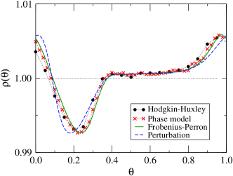
Figure 8: Stationary phase PDFs of the Hodgkin-Huxley neural oscillator driven by external impulses obtained by (i) direct simulation of the original model, (ii) direct simulation of the corresponding phase model, (iii) numerical solution of the corresponding Frobenius-Perron equation, and (iv) perturbation theory using Fourier coefficients numerically obtained from the phase map.

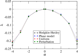
Figure 9: Lyapunov exponent $\lambda$ obtained as a function of the impulse intensity $\sigma$. by (i) directly using the original model, (ii) directly using the reduced phase model, (iii) a calculation using numerical phase maps assuming uniform phase PDF, and (iv) a calculation using numerical phase maps and the approximated phase PDF.

VI Summary

We analyzed phase synchronization of general limit-cycle oscillators subject to external impulses by reducing the dynamics of the oscillator to a random phase map. We proved that when the phase maps are strictly monotonic and the mean inter-impulse interval of the input current is sufficiently large, the Lyapunov exponent of the system always becomes negative, leading to fluctuation-induced phase synchronization. We also treated the case where the inter-impulse interval is finite perturbatively for weak Poissonian impulses, and proved that the next order correction to the upper bound of the Lyapunov exponent is also zero, hence the fluctuation-induced phase synchronization persists even if the phase distribution becomes slightly non-uniform.

Mathematically, the non-positivity of the Lyapunov exponent is a general result of the concavity of the $\log$ function and the monotonicity and periodicity of the phase map. Therefore, this result is not restricted to specific oscillators, but also holds generally for a wide variety of limit-cycle oscillators. Examining the significance of our results in practical problems would be an interesting topic.

Though we did not derive in this paper, we can reduce the phase model driven by Poissonian impulses to an Ito-Langevin phase equation in the limit of weak and frequent impulses when the net drift induced by the external impulses vanishes. It yields

$$\dot{\theta}(t)=\omega+{\bf Z}(\theta)\cdot\bm{\eta}(t),$$ (122)

where $\bm{\eta}(t)$ is a $n$-dimensional Gaussian-white noise. However, it can be shown that the phase disturbance is neutrally stable for this Ito-Langevin phase model, namely, the Lyapunov exponent is constantly zero Teramae , as a direct consequence of the Ito stochastic integral Gardiner . Therefore, if we take the Langevin limit within our phase model, fluctuation-induced phase synchronization does not occur. On the other hand, if the above Langevin phase equation is interpreted in the Stratonovich sense, which does not come out of the integration rule of the impulsive force we assumed in this paper, the phase synchronization occurs Teramae . Thus, slight difference in the treatment of the stochastic forcing leads to physically distinct results. Detailed discussions on this point, including the stochastic interpretation of impulsive forcing, will be reported in the future.

- (1) Z. F. Mainen and T. J. Sejnowski, Science 268 1503 (1995).
- (2) R. R. de Ruyter van Steveninck, G. D. Lewen, S. P. Strong, R. Koberle, W. Bialek, Science, 275 1805 (1997).
- (3) Y. Tsubo, T. Kaneko. S. Shinomoto, Neural Networks 17 165 (2004).
- (4) R. V. Jensen, Phys. Rev. E. 58 R6907 (1998).
- (5) E. K. Kosmidis and K. Pakdaman, J. Comput. Neurosci. 14 5 (2003).
- (6) K. Pakdaman, Neural Comput. 14 781 (2002).
- (7) B. Gutkin, G. B. Ermentrout, and M. Rudolph, J. Comput. Neurosci. 15 91 (2003).
- (8) J. Ritt, Phys. Rev. E 68 041915 (2003).
- (9) J. M. Casado and J. P. Baltanás, Int. J. Bif. and Chaos 14 2061 (2004).
- (10) J. N. Teramae and D. Tanaka, Phys. Rev. Lett. 93 204103 (2004).
- (11) K. Nagai, H. Nakao, and Y. Tsubo, Phys. Rev. E 71 036217 (2005).
- (12) D. S. Goldobin and A. Pikovsky, Phys. Rev. E 71 045201(R) (2005); Physica A 351 126 (2005).
- (13) A. T. Winfree, The Geometry of Biological Time (Springer-Verlag, New York, 2001, 1980).
- (14) Y. Kuramoto, Chemical Oscillations, Waves, and Turbulence (Springer-Verlag, Berlin, 1984).
- (15) A. Pikovsky, M. Rosenblum, and J. Kurths, Synchronization (Cambridge University Press, Cambridge, 2001).
- (16) D. L. Snyder, Random Point Processes (John Wiley & Sons, New York, 1975).
- (17) P. Hänggi, Z. Physik B 31, 407 (1978); Z. Physik B 36, 271 (1980).
- (18) A. Lasota and M. C. Mackey, Probabilistic properties of deterministic systems (Cambridge University Press, New York, 1985).
- (19) L. M. Pecora and T. L. Carroll, Phys. Rev. A 44 2374 (1991).
- (20) A. S. Pikovsky, Phys. Lett. A 165 33 (1992).
- (21) P. Khoury, M. A. Lieberman, and A. J. Lichtenberg, Phys. Rev. E. 54 3377 (1996).
- (22) R. Toral, C.R. Mirasso, E. Hernández-García, O. Piro, in Unsolved Problems on Noise and Fluctuations, UPoN’99, D. Abbot and L. Kiss, eds. AIP Conference Proceedings 511, 255 (2000).
- (23) C. W. Gardiner, Handbook of Stochastic Methods (Springer, Berlin, 1997).
- (24) C. Koch, Biophysics of Computation (Oxford University Press, Oxford, 1999).