Bistability in sine-Gordon: the ideal switch

Abstract

The sine-Gordon equation, used as the representative nonlinear wave equation, presents a bistable behavior resulting from nonlinearity and generating hysteresis properties. We show that the process can be understood in a comprehensive analytical formulation and that it is a generic property of nonlinear systems possessing a natural band gap. The approach allows to discover that sine-Gordon can work as an ideal switch by reaching a transmissive regime with vanishing driving amplitude.

I Introduction

A nonlinear medium submitted to wave irradiation at a frequency in a forbidden band gap can undergo bistable behavior and present hysteresis properties. This bistability has attracted much attention, e.g. in nonlinear optics as a means for a medium to switch from total reflection to partial (sometimes total) transmission winful , or in superconducting junction devices as a means to conceive amplifiers that “remain efficient in the quantum limit” dyn-bif .

We attempt to give here a comprehensive interpretation of this phenomenon in terms of both analytical description and numerical simulations, in order to unveil a particular stationary regime presenting a non-zero output for vanishing input, what we call the ideal switch and which allows for detection of (almost) vanishing signal.

To that end we consider the sine-Gordon equation on the finite interval $x\in[0,L]$

$$u_{tt}-u_{xx}+\sin u=0,$$ (1)

associated to the boundary value problem

$$u(0,t)=f(t),\quad u_{x}(L,t)=0,$$ (2)

on a vanishing initial state (with $f(0)=0$ and $f_{t}(0)=0$ for compatibility of the initial and boundary values).

This is a quite standard problem in physics of a wave equation with a forced extremity (Dirichlet boundary condition in $x=0$) and a free end (Neumann boundary condition in $x=L$), associated to Cauchy initial data at $t=0$. A related physical situation is for instance a long Josephson junction agarwal ; ustinov or an array of coupled short junctions (Josephson superlattice) remoiss ; olsen . Note that, depending on the used external driving, the boundary (2) has possibly to be replaced with $u_{x}(0,t)$.

An important subclass of boundary $f(t)$ is constant amplitude periodic driving at a frequency in the natural band gap of the system, namely

$$f(t)=B_{0}\,\cos(\Omega t),\quad\Omega<1,$$ (3)

after a convenient transient sequence where $f(t)$ grows from a vanishing amplitude to the value $B_{0}$ to avoid initial shock. While for a linear system this boundary excitation does not flow through, nonlinearity allows for energy transmission above the threshold amplitude which reads (in the semi-infinite case $L\to\infty$)

$$B_{s}=4\arctan(b_{s}),\quad b_{s}^{2}=\frac{1-\Omega^{2}}{\Omega^{2}}.$$ (4)

This is called nonlinear supratransmission geniet and happens by emission of solitons (moving breathers) that propagate in the nonlinear medium.

This process, quite generic, has been experimentally realized on a chain of coupled pendula supratrans , and applies for instance in discrete systems of coupled waveguide arrays ramaz where the forbidden gap results from discreteness, or else in Bragg media (periodic dielectric structures) under constant micro-wave irradiation in the photonic band gap bragg . In Josephson junctions arrays, submitted to microwave excitation, the boundary $u_{x}(0,t)=f(t)$ induces the threshold $B_{s}=2(1-\Omega^{2})$ supratrans .

In the finite line case considered here, we shall again find a nonlinear supratransmission threshold which tends to the value (4) for large $L$. But a property far less understood is the hysteresis loop obtained by decreasing the amplitude excitation $B_{0}$ from the threshold $B_{s}$. This property has been for instance observed on numerical simulations remoiss ; olsen in the context of Josephson superlattices, but both the analytical expression of the threshold and the very nonlinear mechanism involved have not been clarified.

We shall establish a general procedure to determine the threshold by studying the standing periodic solutions of sine-Gordon which synchronize to the driving frequency $\Omega$ and adapts to the driving amplitude $B_{0}$. Although these two conditions are sufficient to determine completely the solution, it is not uniquely defined. Indeed we shall prove that a fixed set of physical parameters $\{L,\ \Omega,\ B_{0}\}$ may be related to more than one solution. This is the principle that leads to bistability when $B_{0}<B_{s}$.

As an interesting consequence we obtain that there exists a regime where a vanishing input amplitude $B_{0}$ produces a non-vanishing output amplitude. This process shows that sine-Gordon can be thought of as an ideal switch along the hysteresis loop from zero to zero input amplitudes.

The paper is organized as follows: in the next section we display the set of explicit solutions to sine-Gordon on a length $L$ submitted to the only requirements that the input boundary amplitude be $B_{0}$ and the period of the solution be $2\pi/\Omega$. The following section is devoted to the analytical definition and evaluation of the threshold of bistability. Then we show by numerical simulations in section 4 that those explicit solution are indeed produced by the boundary driving (3) and we check bistability predictions. In particular we compute, for a more realistic damped sine-Gordon model, the power released by the boundary driver to the medium and find that after having switched, this power is 2 to 3 orders of magnitude larger than before the switch.

II Explicit solutions

II.1 General expressions.

Under boundary condition (3), in order to describe the periodic asymptotic regime reached in numerical simulations, we follow scott and seek a solution

$$u(x,t)=4\arctan[X(x)T(t)].$$ (5)

The boundary condition in $u_{x}(L,t)=0$ then reads

$$X^{\prime}(L)=0,\quad X(L)=A,$$ (6)

where we have defined the amplitude parameter $A$ such as to scale $T(t)$ to unity, in other words

$$\exists t_{0}\ :\ T^{\prime}(t_{0})=0,\quad T(t_{0})=1.$$ (7)

By inserting expression (5) in the sine-Gordon equation (1) and by use of constraints (6) and (7), we obtain differential equations with a unique free parameter $\alpha$:

$$(X^{\prime})^{2}=\alpha\Gamma(A^{2}-X^{2})(X^{2}+\frac{1}{\Gamma A^{2}}),$$ (8)

$$(T^{\prime})^{2}=\alpha(1-T^{2})(T^{2}+\Gamma),$$ (9)

where prime denotes differentiation and where

$$\Gamma=\frac{1}{A^{2}}+\frac{1}{\alpha(1+A^{2})}.$$ (10)

Thanks to (6) and (7) the equation for $X(x)$ is integrated on $[x,L]$ and the one for $T(t)$ on $[t,t_{0}]$ . The solution is then completely defined (in terms of elliptic integrals) by the values of the two parameters $A$ and $\alpha$, determined as follows.

Our first fundamental hypothesis is to assume, accordingly with numerical simulations, that the solution synchronizes to the boundary driving, namely that the function $T(t)$ is periodic with the period of the driver:

$$T(t+\frac{2\pi}{\Omega})=T(t).$$ (11)

The second fundamental hypothesis consists in expressing that the solution adapts to the driving amplitude $B_{0}=4\arctan(a)$, which gives

$$X(0)=a.$$ (12)

The two relations (11) and (12) constitute a closed system of equations for the two unknowns $A$ and $\alpha$ in terms of the physical constants $a$, $\Omega$ and $L$.

The point is that bistability occurs because the solution of (8)(9) drastically depends on the sign of $\alpha$. We shall indeed discover that there may exist different solutions that do synchronize to $\Omega$ and adapts to $a$. In other words, for any fixed $\Omega$ and $L$, a given input amplitude $a$ may correspond to more than one value of the output amplitude $A$ as depicted on fig.1.

II.2 Type I solutions.

We call type I solutions those obtained for $\alpha>0$ (implying $\Gamma>0$) for which we obtain byrd

$$T(t)=\rm cn(\omega(t-t_{0}),\nu),$$ (13)

$$X(x)=A\ \rm cn(k(x-L),\mu),$$ (14)

$$\omega^{2}=\alpha(1+\Gamma),\quad\nu^{2}=\frac{1}{1+\Gamma},$$

$$k^{2}=\alpha\Gamma(A^{2}+\frac{1}{\Gamma A^{2}}),\quad\mu^{2}=\frac{\Gamma A^{4}}{1+\Gamma A^{4}}.$$ (15)

where $\rm cn(\cdot,m)$ is the cosine-amplitude Jacobi elliptic function of modulus $m$. According to scott , the resulting solution $u(x,t)$ is called plasma oscillation and we have from (15)

$$\omega^{2}=k^{2}+\frac{1-A^{2}}{1+A^{2}}.$$ (16)

This relation between the nonlinear wave parameters $\omega$ and $k$ is often called a nonlinear dispersion relation but we shall reserve such a denomination to the true dispersion relation which relates the actual period $4{\mathbb{K}}(\mu)/k$ of $X(x)$ to the period $4{\mathbb{K}}(\nu)/\omega$ of $T(t)$.

The parameters $\alpha$ and $A$ are now determined by requiring synchronization (11) and input datum (12), namely here by solving for unknowns $\alpha$ and $A$ the system

$$\Omega\ {\mathbb{K}}(\nu)=\frac{\pi}{2}\ \omega,\quad a=A\ \rm cn(kL,\mu).$$ (17)

(Note: the complete elliptic integral ${\mathbb{K}}(\nu)$ is well defined as for $\Gamma>0$ we have $0<\nu^{2}<1$.)

It is useful to express the above solution in terms of the two wave parameters $\omega$ and $k$. This is done by using (16) to eliminate $A$ and $\alpha$ from the definitions of $\mu$ and $\nu$. We get

$$A^{2}=\frac{1-\omega^{2}+k^{2}}{1+\omega^{2}-k^{2}},$$

$$\nu^{2}=\frac{k^{4}-(\omega^{2}-1)^{2}}{4\omega^{2}},$$ (18)

$$\mu^{2}=\frac{4k^{2}}{(1+k^{2})^{2}-\omega^{4}}.$$

System (17) appears then as an equation for the determination of the parameters $\omega$ and $k$ from the data of the length $L$, the boundary driver’s frequency $\Omega$ and amplitude $a$.

II.3 Type II solutions.

New types of solutions are obtained for $\alpha<0$ for which the evolution (9) of $T(t)$ requires $\Gamma<0$ in order to guarantee the constraint (7). Defining then

$$\beta=-\alpha,\quad\Lambda=-\Gamma=\frac{1}{\beta(1+A^{2})}-\frac{1}{A^{2}},$$ (19)

the basic equations (8) and (9) become

$$(T^{\prime})^{2}=\beta(1-T^{2})(\Lambda-T^{2}),$$ (20)

$$(X^{\prime})^{2}=\beta\Lambda(A^{2}-X^{2})(X^{2}-\frac{1}{\Lambda A^{2}}).$$ (21)

It appears that the constraint (7) which states that $T(t_{0})=1$, requires $\Lambda>1$, namely

$$\beta<\frac{A^{2}}{(1+A^{2})^{2}},$$ (22)

a condition that must be checked a posteriori when computing $\beta$ from the synchronization constraint.

The structure of the equation (21) implies two classes of solutions depending on the relative values of $A^{2}$ and $1/(\Lambda A^{2})$. Type II solutions are obtained for $\Lambda A^{4}>1$ which, together with constraint (22), reads

$$A^{2}>1\ :\ 0<\beta<A^{2}/(1+A^{2})^{2},$$ (23)

$$A^{2}<1\ :\ 0<\beta<A^{4}/(1+A^{2})^{2},$$ (24)

The solution of (20)(21) can now be obtained as

$$T(t)=\rm sn(\omega(t-t_{1}),\nu),\quad t_{1}=t_{0}+{\mathbb{K}}(\nu)/\omega$$ (25)

$$X(x)=A\ \rm dn(k(x-L),\mu),$$ (26)

$$\omega^{2}=\beta\Lambda,\quad\nu^{2}=\frac{1}{\Lambda},$$

$$k^{2}=\beta\Lambda A^{2},\quad\mu^{2}=1-\frac{1}{\Lambda A^{4}},$$ (27)

and we have the relation

$$\omega^{2}=\frac{k^{2}}{A^{2}},$$ (28)

between the wave parameters $k$ and $\omega$ for type II solution.

The parameters $\beta$ and $A$ are determined as before by requiring synchronization (11) and input datum (12), namely

$$\Omega\ {\mathbb{K}}(\nu)=\frac{\pi}{2}\ \omega,\quad a=A\ \rm dn(kL,\mu).$$ (29)

Although the above equation, for real valued parameters, has two sets of solutions $\{\beta,A\}$, only one set verifies the constraint $\Lambda A^{4}>1$.

As before, we express the type II solution in terms of the wave parameters $\omega$ and $k$, by means of (28) to eliminate $A$ and $\beta$ in $\mu$ and $\nu$. We obtain

$$A^{2}=\frac{k^{2}}{\omega^{2}},$$

$$\nu^{2}=\frac{k^{2}}{\omega^{2}}\,\frac{1-\omega^{2}-k^{2}}{\omega^{2}+k^{2}},$$ (30)

$$\mu^{2}=1-\frac{\omega^{2}}{k^{2}}\,\frac{1-\omega^{2}-k^{2}}{\omega^{2}+k^{2}}.$$

System (29) determines then the parameters $\omega$ and $k$ from the data of $L$, $\Omega$ and $a$.

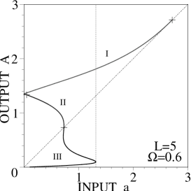
Figure 1: Plot of the curves $|A(a)|$ in the three cases for $L=5$ and $\Omega=0.6$. The crosses indicate the points where the solution changes from one type to the other. The vertical line shows the threshold amplitude $a_{s}$ (next section) above which supratransmission occurs by emission of solitons.

II.4 Type III solutions.

The type III solution is obtained still for $\alpha<0$ when $\Lambda A^{4}<1$. Such can be realized only in the case $A^{2}<1$ by requiring

$$A^{4}/(1+A^{2})^{2}<\beta<A^{2}/(1+A^{2})^{2}.$$ (31)

The solution of (20)(21) now reads

$$T(t)=\rm sn(\omega(t-t_{1}),\nu),\quad t_{1}=t_{0}+{\mathbb{K}}(\nu)/\omega$$ (32)

$$X(x)=A\,\rm dn^{-1}(k(x-L),\mu),$$ (33)

$$\omega^{2}=\beta\Lambda,\quad\nu^{2}=\frac{1}{\Lambda},\quad k^{2}=\frac{\beta}{A^{2}},\quad\mu^{2}=1-\Lambda A^{4},$$ (34)

and the wave parameters obey

$$\omega^{2}=\frac{1}{1+A^{2}}-k^{2}.$$ (35)

The synchronization condition (11) and input datum (12) furnish here the system

$$\Omega\ {\mathbb{K}}(\nu)=\frac{\pi}{2}\ \omega,\quad a=\frac{A}{\rm dn(kL,\mu)}.$$ (36)

for the unknowns parameters $\beta$ and $A$. The same remark as for the type II solution holds here, namely that the system (36) has two sets of solutions $\{\beta,A\}$ but only one verifies the constraint $\Lambda A^{4}<1$.

Again the type III solution can be expressed entirely in terms of the two parameters $\omega$ and $k$ by means of (35) which gives

$$A^{2}=\frac{1-\omega^{2}-k^{2}}{\omega^{2}+k^{2}},$$

$$\nu^{2}=\frac{k^{2}}{\omega^{2}}\,\frac{1-\omega^{2}-k^{2}}{\omega^{2}+k^{2}},$$ (37)

$$\mu^{2}=1-\frac{\omega^{2}}{k^{2}}\,\frac{1-\omega^{2}-k^{2}}{\omega^{2}+k^{2}}.$$

Then (36) is a system for the parameters $\omega$ and $k$ in terms of the data $L$, $\Omega$ and $a$.

III Bistability thresholds

The above 3 solutions are now used to describe analytically bistability properties of sine-Gordon. The first step is to define and calculate, at given length $L$, the threshold $a_{s}$ as functions of the driving frequency $\Omega$. Last, decreasing the input amplitude from $a_{s}$, once a transmission regime has been reached, the system locks to the type-I solution which holds down to a vanishing driving amplitude. This is a property that makes sine-Gordon as the ideal switch and allows to understand how it can be used to amplify weak (vanishing) signals.

III.1 Transmission threshold

As shown by figure 1, increasing the input amplitude from $a=0$ generates the type III solution. This solution has a maximum input value $a_{s}$ resulting from (36) as the point where $\rm dn(kL,\mu)$ reaches its minimum value $\sqrt{1-\mu^{2}}$, namely

$$a_{s}^{2}=\frac{A^{2}}{1-\mu^{2}}.$$ (38)

Such a definition of the threshold $a_{s}$ is more conveniently written in terms of $\omega$ and $k$ through (II.4) as

$$a_{s}^{2}=\frac{k^{2}}{\omega^{2}}.$$ (39)

In this equation, the parameters $\omega$ and $k$ are determined through (36), which, at the threshold, can also be written as the system

$$\Omega\ {\mathbb{K}}(\nu)=\frac{\pi}{2}\ \omega,\quad kL={\mathbb{K}}(\mu),$$ (40)

with $\nu$ and $\mu$ given by (II.4).

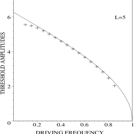
Figure 2: Input amplitude $4\arctan(a_{s})$ at the threshold, solution of (39)(40) as a function of $\Omega$ for $L=5$ (crosses) and compared to its limit value $4\arctan(b_{s})$ as $L\to\infty$, given by (43) (full line).

The figure 2 shows that the threshold $a_{s}$ is quite close to the expression of $b_{s}$ in (4). This property is demonstrated in general by studying the limit $L\to\infty$ in the type III solution. At threshold amplitude, the relation (40) between $L$ and $\mu$ gives the necessary condition

$$L\to\infty\ \Rightarrow\ \mu\to 1\ \Rightarrow\ \omega^{2}\to 1-k^{2},$$ (41)

with which the synchronization condition provides

$$L\to\infty\ \Rightarrow\ \nu\to 0\ \Rightarrow\ \omega\to\Omega.$$ (42)

With this in hands, the expression (39) of the threshold readily gives the expression (4), namely

$$L\to\infty\ \Rightarrow\ a_{s}^{2}\to b_{s}^{2}=\frac{1-\Omega^{2}}{\Omega^{2}}.$$ (43)

Remark: it is instructive to compute also the limit $L\to\infty$ on the solution itself at the threshold where from (II.4) and (41) obviously $A\to 0$. In that case we rewrite the solution $X(x)$ of (33) as

$$X(x)=\frac{a\,\rm dn(kL,\mu)}{\rm dn(k(x-L),\mu)},$$ (44)

expand the denominator, take the limit $L\to\infty$ first and make then $\mu\to 1$. We obtain $X(x)$ of (33) as

$$X(x)\underset{L\to\infty}{\longrightarrow}a_{s}\,\rm sech(kx).$$ (45)

The same procedure applied to $T(t)$ in (32), with $\nu\to 0$, provides

$$T(t)\underset{L\to\infty}{\longrightarrow}\cos(\omega(t-t_{0})),$$ (46)

Figure 3: Output amplitude $4\arctan(A)$ when $a=0$ as a function of $\Omega$ for $L=5$ obtained from (48) by solving (47).

and the resulting solution $u(x,t)$ of sine-Gordon on the semi-line is the stationnary breather centered in $x=0$ accordingly with geniet .

III.2 Ideal switch

Considering the type I solution, expression (17) that links the input $a$ to the output $A$ can produce $a=0$ with $A\neq 0$, such as to generate a regime of non-vanishing output value with a vanishing input amplitude, the ideal switching regime. This is the case when

$$kL={\mathbb{K}}(\mu),\quad\Omega\ {\mathbb{K}}(\nu)=\frac{\pi}{2}\ \omega.$$ (47)

where $A$, $\mu$ and $\nu$ are related to $\omega$ and $k$ through (II.2). Note the formal analogy with (40) where the parameters $A$, $\mu$ and $\nu$ are different.

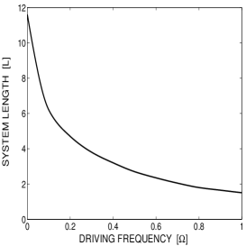
Figure 4: Minimal length of the system below which one does not have ideal switch (the solution of (47) ceases to exist).

This is a system of equations for $\{\omega,k\}$ whose solution then produces the seeked output amplitude by

$$A^{2}=\frac{1-\omega^{2}+k^{2}}{1+\omega^{2}-k^{2}},$$ (48)

defined by (47) in terms of the physical entries $L$ and $\Omega$. We have plotted in fig.3 the output amplitude $4\arctan A$ in the ideal switching case ($a=0$) as a function of $\Omega$ for length $L=5$.

We observe that, for a given length, there exists a threshold in frequency below which no ideal switching is allowed. This is understood by observing that $A^{2}$ diverges when $\omega^{2}\to k^{2}-1$, for which $\mu\to 1$ (a limit threshold that has exactly the same origin as in (41) when $L\to\infty$). Conversely, at given driver frequency $\Omega$, there exists a minimum length $L$ of the medium to obtain an ideal switch, it is displayed on fig. 4.

Let us remark that the notion of nonlinear dispersion relation is not useful to predict, at given driving frequency $\Omega$, the minimum driver amplitude that generates transmission, as indeed we have here an example where this minimum is simply vanishing.

IV Numerical simulations

IV.1 Damping and boundary driving.

Bistable properties, and in particular ideal switching, have been analytically described in the integrable case (1). However, any realistic physical situation must take into account the damping inherent to the medium. The simplest way to include damping is to assume the model

$$u_{tt}+\gamma u_{t}-u_{xx}+\sin u=0,$$ (49)

associated with the initial-boundary value problem (2) in the particular subclass (3). We study here the bistable properties of (49) by numerical simulations and compare the results to the analytical predictions.

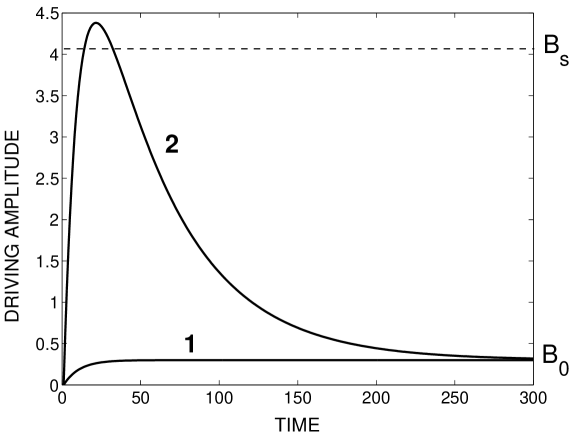
Figure 5: Two different paths for driving the sine-Gordon system. $B_{0}$ is the driving amplitude in stationary regime and $B_{s}$ is a supratransmission threshold.

To that end the system is driven at the input boundary $x=0$ with a bandgap frequency and time dependent amplitude as follows: in a first numerical simulation, the amplitude is smoothly increased up to the value $B_{0}$ smaller than the supratransmission threshold $B_{s}$. In a second simulation, the amplitude is increased up to a value exceeding the supratransmission threshold and then, after a time sufficient to generate moving breathers, it is decreased to the same value $B_{0}$ as in the first case. The figure 5 displays the two time variations of the driving amplitude that we have used in the numerical simulations. After having reached a stationary regime, although the driving amplitudes $B_{0}$ are equal in both cases, the dynamics drastically differ in those two cases as it is expected from the analytical consideration presented above and described hereafter.

IV.2 Evidence of bistability.

In most of our numerical simulations we choose the driving frequency in the middle of the band gap $\Omega=0.5$, use damping parameter $\gamma=0.01$ and length $L=4.1$. For the driving amplitude along path 1 in fig.5, we always observe a stationary regime with decaying profile of the standing wave, very well described by the exact analytical solution of type III (32)(33). Instead, when driving along path 2, we get the picture corresponding to the exact type I solution (13)(14). Those two drastically different behaviors of the system are displayed as three dimensional plots in fig.6.

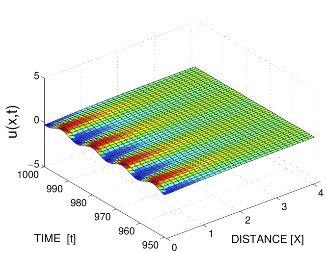
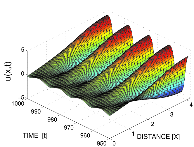
Figure 6: Three dimensional plots of the sine-Gordon system dynamics after having reached stationary regime. Upper plot corresponds to the driving path 1 of fig.5 and lower plot to path 2. In both cases driving frequency is $\Omega=0.5$, stationary driving amplitude $B_{0}=0.3$, damping coefficient $\gamma=0.01$ and system length $L=4.1$.

It is remarkable on the second picture of fig.6 that the system has locked to a stationary solution with a small driving amplitude (here $B_{0}=0.3$) and a large output amplitude (evaluated at $B=4.35$). Let us mention that we can drive the system with amplitudes down to $B_{0}=0.1$ and still have the type I solution (large output amplitude) despite presence of damping in the system, getting thus a regime of almost ideal switch, or almost perfect detector.

Another remark is that the system never locks to the exact solution of type II (25)(26), simply because this solution is unstable. For instance, if that exact solution is used as an initial condition in sine-Gordon, it eventually breaks down.

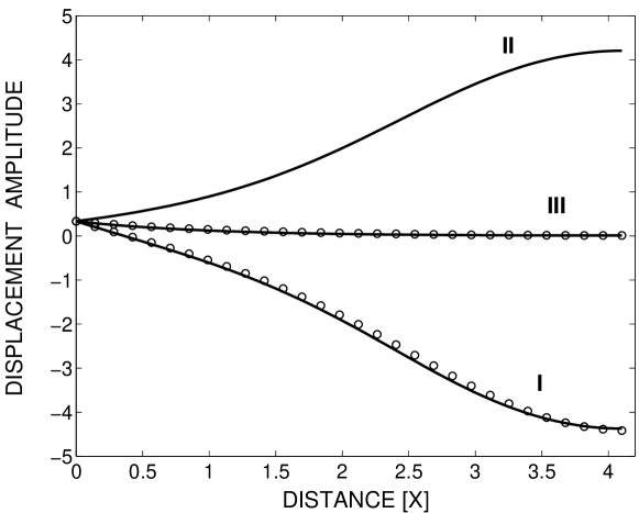
Figure 7: Comparison of analytical expressions (solid lines) for the profiles of standing waves (33), (26), (14), corresponding to solutions of type III, II and I respectively, and numerical simulations (circles). The type III solution is reached along path 1 of fig. 5 while the type I results from path 2. The type II solution, unstable, is never reproduced by the system.

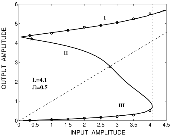
Figure 8: Comparison of input-output amplitude dependence obtained from numerical simulations (circles) with analytical curves derived from formulas (17), (29), (36).

To be complete, we compare the analytical expressions of the standing waves profiles of (33), (26) and (14) to the results of numerical simulations in the case of the two different driving paths in the context of fig.6. The result is displayed in figure 7 where the obtained perfect matching shows that indeed the system locks to the analytical solution obtained by assuming frequency synchronization and amplitude matching. This is completed by plotting in fig.8 the input-output amplitude dependence obtained from numerical simulations and its comparison with analytical curves derived from formulas (17), (29) and (36).

IV.3 Energetic considerations.

The physically useful bistable nature of the system manifests in large difference between the energy dissipation in the two stationary regimes. The averaged energy released from the driver in unit time, can be expressed as

$$P=\frac{\Omega}{2\pi}\int\limits_{0}^{2\pi/\Omega}dt\int\limits_{0}^{L}dx\ \gamma\,u_{t}^{2}.$$ (50)

Indeed one can easily obtain

$$\frac{\partial}{\partial t}\int\limits_{0}^{L}dx\,{\cal H}=-\int\limits_{0}^{L}dx\,\gamma\,u_{t}^{2}-\left.(u_{x}u_{t})\right|_{x=0},$$

$${\cal H}=\frac{1}{2}u_{t}^{2}+\frac{1}{2}u_{x}^{2}+1-\cos u,$$ (51)

which by averaging on one period furnishes (50) as the boundary value in $x=0$ is periodic.

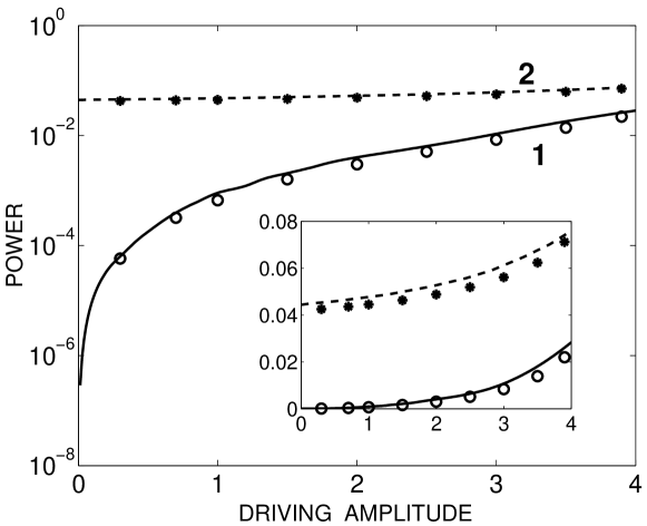
Figure 9: Power $P$ of (50) in terms of the driving amplitude in lin-log (main plot) and lin-lin (inset) scales. Solid line (solution (13,14)) and circles (simulations) correspond to driving regime 1 of fig.5. Dashed line (solution (32,33)) and asterisks (simulations) result from driving regime 2. Length is $L=4.1$, driving frequency $\Omega=0.5$ and damping coefficient $\gamma=0.01$.

Although the analytical solution of the sine-Gordon equation (1) are not solutions of the damped version (49), we may compare the power defined above obtained by numerical simulations of (49) to the expression (50) where $u$ is simply replaced by the exact solution (type III before the switch, type I after). The result of this comparison is displayed in fig.9 wher we see that expression (50) with analytical solutions fit strikingly well the numerical simulations, and that the power $P$ after the switch is two to three orders of magnitude greater than before the switch.

V Comments and conclusion.

It is worth mentioning that while the analytical solution of type I holds for any length $L$, in a realistic physical system (nonzero damping), the situation is different. In particular, for large L and low driving amplitudes, when several nodes of type I standing wave solution are present, the solution cannot survive and decays to type III solution. This is understood by the following simple argument: all of the exact solutions derived in the previous sections are standing waves, i.e. they do not generate energy flux. Thus, regions of the system far from the boundary cannot gain energy from the driver and the oscillations will eventually fade away.

We have essentially demonstrated, both by analytical and numerical treatment, that the bistable property on the sine-Gordon system allows to generate a particular regime that works as an ideal switch: nonzero output for vanishing input. In a realistic physical system (including damping) the property is conserved but for small (non-vanishing) input. This nonlinear hysteretis has been shown to correspond to quite determinant differences in the power released by the driver to the system.

acknowledgements: It is a pleasure to thank Yu.S. Kivshar for the useful information regarding the recent experiments on bifurcations in Josephson junctions. One of us (R.Kh.) aknowledge support of the France-NATO visiting scientist fellowship award.

References

- (1) H.G. Winful, J.H. Marburger, E. Garmire, Appl Phys Lett 35 (1979) 379
- (2) I. Siddiqi, R. Vijay, F. Pierre, C.M. Wilson, L. Frunzio, M. Metcalfe, C. Rigette, R.J. Schoelkopf, M.H. Devoret, D. Vion, D. Esteve, Phys Rev Lett 94 (2005) 027005
- (3) S.R. Shenoy, G.S. Agarwal, Phys Rev Lett 44 (1980) 1524
- (4) A.V. Ustinov, Physica D 123 (1998) 315
- (5) D. Barday, M. Remoissenet, Phys Rev B 41 (1990) 10387
- (6) Yu.S. Kivshar, O.H. Olsen, M.R. Samuelsen, Phys Lett A 168 (1992) 391
- (7) F. Geniet, J. Leon, Phys Rev Lett 89 (2002) 134102
- (8) F. Geniet and J. Leon, J Phys: Cond Matt 15 (2003) 2933
- (9) R. Khomeriki, Phys Rev Lett 92 (2004) 063905
- (10) J. Leon, A. Spire, Phys Lett A 327 (2004) 474
- (11) G. Costabile, R.D. Parmentier, B. Savo, D.W. McLaughlin, A.C. Scott, Appl Phys Lett 32 (1978) 587
- (12) P.F. Byrd, M.D. Friedman, Handbook of elliptic integrals for engineers and physicists, Springer (Berlin 1954)