Resonance-assisted tunneling in three degrees of freedom without discrete symmetry

Abstract

We study dynamical tunneling in a near-integrable Hamiltonian with three degrees of freedom. The model Hamiltonian does not have any discrete symmetry. Despite this lack of symmetry we show that the mixing of near-degenerate quantum states is due to dynamical tunneling mediated by the nonlinear resonances in the classical phase space. Identifying the key resonances allows us to suppress the dynamical tunneling via the addition of weak counter-resonant terms.

Tunneling is a phenomenon that is forbidden by classical mechanics but allowed by quantum mechanics. In general, any flow of quantum probability between (approximately) equivalent yet classically disconnected regions constitutes tunneling. The classical regions could be disconnected due to barriers in coordinate space, momentum space or, more generally, in the classical phase space. In the cases where tunneling occurs despite the absence of obvious energetic barriers it is called dynamical tunnelingdavhel ; the barriers now arise due to certain exact or approximate constants of the motion and hence are naturally identified in the underlying classical phase space. Considerable theoreticaldavhel ; cats ; cat1 ; frido ; rat1 ; rat2 ; ozo ; ejhsar ; elt ; self and experimentalexpt works have established that tunneling between quantum states localized on two symmetry-related regions in the phase space can be strongly influenced by the classical stochasticity (chaos-assisted tunnelingcats ) and/or by the intervening nonlinear resonances (resonance-assisted tunnelingrat2 ). In the former case, phase space is mixed regular-chaotic and the splittings show marked dependence on the nature of the chaotic states which couple to the tunneling doubletscats ; cat1 ; frido . In the latter case with near-integrable phase space, the splittings depend delicately on the various resonance islands bridging the degenerate statesrat1 ; rat2 ; ozo ; ejhsar ; elt ; self . Clearly, a quantitative semiclassical theory, still elusive, requires one to identify key structures in the phase space on which the theory is to be based. In this regard there is increasing evidenceelt ; self that the classical nonlinear resonances might play a central role in near-integrable as well as mixed phase space situations.

However, most of the studies thus far have been on two degrees of freedom (dof) systems with discrete symmetriesexcep . Does the resonance-assisted tunneling viewpoint hold in systems with three or more dof which lack discrete symmetries? The main motivation for our study comes from suggestionsejhsar put forward in the molecular context - can dynamical tunneling provide a route for mixing between near-degenerate states and hence energy flow between regions supporting qualitatively different types of motion? In addition, notwithstanding the difficulties associated with visualizing the multidimensional phase space, dynamics in three or more dof has features that cannot manifest in the systems studied up until nowlicht . In this letter we attempt to understand dynamical tunneling in a model nonsymmetric, near-integrable three dof system. We show that mixing of near-degenerate states occurs via dynamical tunneling mediated by nonlinear resonances and the mixing can be suppressed by adding weak counter-resonant terms.

We study the Hamiltonian

$$H=H_{0}+\sum_{r}K_{{\bf m}_{r}}[(a_{1}^{\dagger})^{\alpha_{r}}(a_{2})^{\beta_{r}}(a_{3})^{\gamma_{r}}(a_{4})^{\delta_{r}}+{\rm h.c.}],$$ (1)

describing four coupled modes $j=1,2,3,4$ with

$$H_{0}=\sum_{j}(\omega_{j}n_{j}+x_{jj}n_{j}^{2})+\sum_{j<k}x_{jk}n_{j}n_{k},$$ (2)

and $H_{0}|{\bf n}\rangle=E_{\bf n}^{0}|{\bf n}\rangle$. Although eq. 1 has been inspired in the molecular contextquack , similar multiresonant Hamiltonians arise in a variety of systemssimil1 . The occupation number of the $j^{th}$ mode, $n_{j}\equiv a_{j}^{\dagger}a_{j}$, is expressed in terms of the harmonic creation ($a_{j}^{\dagger}$) and destruction ($a_{j}$) operators. The perturbations are characterized by ${\bf m}_{r}=(\alpha_{r},-\beta_{r},-\gamma_{r},-\delta_{r})$ with strengths $K_{{\bf m}_{r}}$. The classical limit of eq. 1, generated via the correspondence $a_{j}\leftrightarrow\sqrt{I_{j}}\exp(i\theta_{j})$, is the following Hamiltonian:

$${\cal H}({\bf I},{\bm{\theta}})={\cal H}_{0}({\bf I})+2\epsilon\sum_{r}K_{{\bf m}_{r}}\sqrt{I_{1}^{\alpha_{r}}I_{2}^{\beta_{r}}I_{3}^{\gamma_{r}}I_{4}^{\delta_{r}}}\cos({\bf m}_{r}\cdot{\bm{\theta}}).$$ (3)

$({\bf I},{\bm{\theta}})$ are the classical action-angle variables of ${\cal H}_{0}$ and hence the perturbations correspond to classical nonlinear resonances. The parameter $\epsilon$ has been introduced for a perturbative analysis (see below). We restrict ourselves to three perturbations ${\bf m}_{1}=(1,-2,0,0)$, ${\bf m}_{2}=(1,-1,-1,0)$, and ${\bf m}_{3}=(1,-1,0,-1)$. This allows for a clear study of the role of the specific resonances in dynamical tunneling. The existence of a conserved quantity $P=n_{1}+(n_{2}+n_{3}+n_{4})/2$, with the classical analog $P_{c}=I_{1}+(I_{2}+I_{3}+I_{4})/2$, implies that the 4-mode system has effectively three dof. The eigenstates, eigenvalues, and the resulting mean level spacing of $H$ are denoted by $|\alpha\rangle$, $E_{\alpha}$ and $\Delta E$ respectively. In the units appropriate for the model Hamiltonianquack the Heisenberg time is given by $\tau_{H}=(2\pi c\Delta E)^{-1}$ with $c$ being the speed of light.

We are interested in the fate of a set of near-degenerate zeroth-order states in the presence of weak perturbations, $K_{{\bf m}_{r}}/\Delta E\equiv k_{{\bf m}_{r}}<1$. Consider states $|{\bf n}\rangle$, $|{\bf n}^{\prime}\rangle$, $|{\bf n}"\rangle,\ldots$ such that $E_{\bf n}^{0}\approx E_{\bf n^{\prime}}^{0}\approx E_{\bf n"}^{0}\approx\ldots$ with average energy $\bar{E}$ and $E_{\bf n}^{0}\in(\bar{E}-\Delta E/2,\bar{E}+\Delta E/2)$. Certain states, among the set of near-degenerate states, mix since they are directly connected to each other via one of the perturbations. The nonlinear resonances in eq. 3 do mediate the mixing via dynamical tunneling. However, in this work we will focus on states that are not directly coupled by the resonances in eq. 3 in order to show that even very weak, induced resonances can lead to substantial mixing that can be associated with dynamical tunneling. Quantum mechanically, the extent of mixing of a zeroth-order state $|{\bf n}\rangle$ can be gauged by computing the survival probability $P_{{\bf n}Q}(t)$ and the inverse participation ratio (IPR) $\sigma_{\bf n}$,

$$P_{{\bf n}Q}(t) = |\langle{\bf n}|e^{-iHt/\hbar}|{\bf n}\rangle|^{2}=\sum_{\alpha,\beta}p_{{\bf n}\alpha}p_{{\bf n}\beta}e^{-i\omega_{\alpha\beta}t},$$ (4)

$$\sigma_{\bf n} = \lim_{T\rightarrow\infty}\frac{1}{T}\int_{0}^{T}P_{{\bf n}Q}(t)dt=\sum_{\alpha}p^{2}_{{\bf n}\alpha},$$ (5)

with $p_{{\bf n}\alpha}=|\langle\alpha|{\bf n}\rangle|^{2}$ and $\omega_{\alpha\beta}=(E_{\alpha}-E_{\beta})/\hbar$. If $\sigma_{\bf n}\ll 1$ then $|{\bf n}\rangle$ mixes extensively with other zeroth-order states.

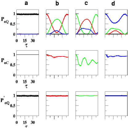
Figure 1: Quantum survival probability (top row) $P_{{\bf n}Q}$ of the states $|{\bf n}\rangle=|0,11,1,4\rangle\equiv|a\rangle$ (black), $|0,11,2,3\rangle\equiv|b\rangle$ (red), $|0,12,2,2\rangle\equiv|c\rangle$ (green), and $|0,13,1,2\rangle\equiv|d\rangle$ (blue). Time $\tau$ is measured in units of the Heisenberg time and $0.5K_{{\bf m}_{1}}=K_{{\bf m}_{2}}=K_{{\bf m}_{3}}\approx 0.2\Delta E$. $\Delta E\approx 4.44$ cm^-1 for eq. 1 with $P=8$. The cross probabilities $|\langle{\bf n}^{\prime}|{\bf n}(t)\rangle|^{2}$ are also shown. The middle row shows the classical analog, $P_{{\bf n}C}$, of $P_{{\bf n}Q}$. $P_{{\bf n}C}$ indicates trapped motion and is qualitatively different from $P_{{\bf n}Q}$. The bottom row shows the quantum $P^{{}^{\prime}}_{{\bf n}Q}$ with the addition of weak counter-resonant terms (eq. 7). The dynamical tunneling essentially shuts down, proving the importance of the induced resonances.

Specifically, we investigate a set of zeroth-order states around $\bar{E}\approx 3542.5\Delta E$ and $P=8$. This choice of $\bar{E}$ is motivated by the existence of a number of near-degenerate states and qualitatively similar behavior is seen at different values of $\bar{E}$ as well. We select states that are not directly coupled by the perturbations in eq. 1 but nevertheless have IPR smaller than one. In Fig. 1 we show the survival probabilities for four such zeroth-order states $|a\rangle=|0,11,1,4\rangle$, $|b\rangle=|0,11,2,3\rangle$, $|c\rangle=|0,12,2,2\rangle$, and $|d\rangle=|0,13,1,2\rangle$ with $\sigma_{\bf n}=0.97,0.51,0.40$, and $0.74$ respectively. The crucial thing to note is that $|b\rangle$,$|c\rangle$, and $|d\rangle$ mix amongst themselves over long times. The corresponding classical calculations, shown in Fig. 1 middle row, indicate long time trapping. Thus the observed mixing between the states is classically forbidden and corresponds to dynamical tunneling. In Fig. 2 the variation of the energy levels with the coupling parameter $k_{{\bf m}_{1}}$ is shown to indicate the lack of avoided crossings between the states of interest. Fig. 2 also shows the spectral intensities $p_{{\bf n}\alpha}$ and in every case we see two clumps of lines - one at the origin and another $\approx 60\Delta E$ away. A purely quantum explanation invokes the second clump of states, the virtual or off-resonance states, which provide a ”vibrational superexchange” pathway for the mixingsuper . The virtual states themselves have $\sigma_{\bf n}\approx 1$ and hence do not mix significantly. It is particularly striking to note that neither $p_{{\bf n}\alpha}$ nor the energy level variations suggest any differences between the zeroth-order states in contrast to the observations in Fig. 1. We now show that a relatively simple explanation can be given in terms of resonance-assisted tunneling on the energy shell.

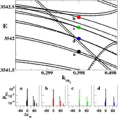
Figure 2: Eigenvalues $E\equiv E_{\alpha}/\Delta E$ versus varying coupling strength $k_{{\bf m}_{1}}\equiv K_{{\bf m}_{1}}/\Delta E$. $K_{{\bf m}_{2}}=K_{{\bf m}_{3}}\approx 0.2\Delta E$. The circles correspond to the eigenstates having the largest contribution from the specific zeroth-order states (Fig. 1). The dotted lines show a similar calculation using eq. 7 indicating no qualitative change in the level motions. The bottom panel shows the overlap intensities $p_{{\bf n}\alpha}=|\langle\alpha|{\bf n}\rangle|^{2}$ versus $\Delta\epsilon_{\bf n}\equiv(E_{\bf n}^{0}-E_{\alpha})/\Delta E$. Note the log-scale for the intensities and the cluster of lines in all the plots around $\Delta\epsilon_{\bf n}=0$, and $60$.

In the resonance-assisted tunneling scenario the mixing between, for example, $|b\rangle$ and $|c\rangle$ can be mediated by a 1:1 resonance involving modes $j=2$ and $4$ i.e., a resonance vector ${\bf m}_{i3}\equiv(0,1,0,-1)$. The Hamiltonian in eq. 3 does not have ${\bf m}_{i3}$ explicitly but it can be induced by ${\bf m}_{1}$ and ${\bf m}_{3}$. Similarly, ${\bf m}_{i1}\equiv(0,0,1,-1)$ and ${\bf m}_{i2}\equiv(0,1,-1,0)$ can be induced by the resonances in eq. 3. The resonances can be visualized by constructing the Arnol’d weblicht at $E\approx\bar{E}$ and fixed $P$, i.e., the intersection of the various resonance planes ${\bf m}_{r}\cdot\partial{\cal H}_{0}({\bf I})/\partial{\bf I}=0$ with the energy shell ${\cal H}_{0}({\bf I})\approx\bar{E}$. For near-integrable systems the energy shell, resonance zones, and the location of the zeroth-order states can be projected onto a $2$-dimensional space of two independent frequency ratios. The “static” Arnol’d web based on ${\cal H}_{0}$ highlights the various possible resonances and their topology on ${\cal H}_{0}({\bf I})\approx\bar{E}$. However, from the tunneling perspective it is crucial to determine dynamically relevant part of the static web at $E\approx\bar{E}$. This “dynamical web” is determined via a wavelet based local frequency analysisarewig of the Hamiltonian eq. 3. Briefly, initial conditions $({\bf I},{\bm{\theta}})$ satisfying ${\cal H}({\bf I},{\bm{\theta}})\approx\bar{E}$ are generated and the trajectories are followed in the frequency ratio space $(\Omega_{1}/\Omega_{3},\Omega_{1}/\Omega_{4})$. The frequencies $\Omega_{k}(t)$ are computed along the trajectory $({\bf I},{\bm{\theta}})(t)$ by performing the wavelet transform of $z_{k}(t)=\sqrt{2I_{k}(t)}\exp(i\theta_{k}(t))$. The total number of visits in a given region of the ratio space gives a density plot representing the web which highlights dynamically significant regions at a given energy. The resulting ”dynamical web” is shown in Fig. 3 along with the location of the relevant zeroth-order states. Apart from highlighting the primary resonances ${\bf m}_{1},{\bf m}_{3}$ the figure also indicates the existence of the induced resonances ${\bf m}_{i1},{\bf m}_{i2}$, and ${\bf m}_{i3}$ separating the states. The states are located close to the junction formed by the three induced resonances and far away from the primary resonances. Hence Fig. 3 supports the notion that $|b\rangle,|c\rangle$, and $|d\rangle$ are mixed due to dynamical tunneling mediated by the induced resonances.

Figure 3: The “dynamical” Arnol’d web at $E=\bar{E}$ generated by propagating $25000$ classical trajectories for $\tau\approx 40$. The primary resonances, ${\bf m}_{1}$ (red), ${\bf m}_{2}$ (black) and ${\bf m}_{3}$ (magenta), as predicted by ${\cal H}_{0}$ are superimposed for comparison. ${\bf m}_{2}$ and ${\bf m}_{3}$ intersect on the energy shell giving rise to the induced resonance ${\bf m}_{i1}=(0,0,1,-1)$. ${\bf m}_{2}$ and ${\bf m}_{3}$ interact with ${\bf m}_{1}$ to give rise to the two other induced resonances ${\bf m}_{i2}=(0,1,-1,0)$ and ${\bf m}_{i3}=(0,1,0,-1)$ respectively. The nearly degenerate zeroth-order states (filled circles) are located close to the induced resonances (arrows) which lead to state-mixing (cf. Fig. 1) via resonance-assisted tunneling.

In order to conclusively establish the role of the induced resonances it is necessary to extract their strengths by perturbativelyrat2 ; ozo ; self removing the primary resonances in eq. 3 to $O(\epsilon)$. As a result we obtain the effective Hamiltonian containing the induced resonances at $O(\epsilon^{2})$ which are approximated by effective pendulums. For instance, one obtains the effective pendulum Hamiltonian

$${\cal H}^{(24)}_{eff}=\frac{(K_{24}-K_{24}^{r})^{2}}{2M_{24}}+2V_{24}\cos 2\phi_{24},$$ (6)

appropriate for the induced resonance $\lambda_{{\bf m}_{i3}}$ with $K_{24}\sim 2I_{4}$ and $2\phi_{24}\sim(\theta_{2}-\theta_{4})$. The resonance center is denoted by $K_{24}^{r}$. The coupling $V_{24}$ can be expressed in terms of the conserved quantities $I_{3},P_{c}$, and $P_{24}\equiv I_{2}+I_{4}$ and the resulting tunneling time $\tau_{tun}\approx(2\pi\Delta E/V_{24})$ agrees well with Fig. 1. The strengths estimated via a pendulum approximation can be translated back to effective quantum strengths $\lambda_{{\bf m}}$ and our analysis reveals that the induced resonances are more than an order of magnitude smaller then that of the primary resonances ($\lambda_{{\bf m}_{i1}}\ll|\lambda_{{\bf m}_{i2}}|\approx|\lambda_{{\bf m}_{i3}}|\approx 0.035K_{{\bf m}_{1}}$). Note that ${\bf m}_{i2}$ and ${\bf m}_{i3}$ come with a negative sign as opposed to ${\bf m}_{i1}$. It is knownrat2 that for significant mixing the states must lie symmetrically with respect to the center of the mediating resonance zone. Among the states considered, $|b\rangle$ and $|c\rangle$ satisfy the criterion very well and hence enhanced mixing between them is seen in Fig. 1. The state $|a\rangle$ is not symmetrically located with respect to $|b\rangle$ and thus, combined with the very small strength $\lambda_{{\bf m}_{i1}}$, the induced resonance ${\bf m}_{i1}$ is ineffective. Now consider modifying eq. 1 according to

$$H^{\prime}=H+|\lambda_{{\bf m}_{i2}}|(a_{2}^{\dagger}a_{3}+{\rm h.c.})+|\lambda_{{\bf m}_{i3}}|(a_{2}^{\dagger}a_{4}+{\rm h.c.}),$$ (7)

where we have added terms to counter the induced resonances. The reasoning is simple - if the induced resonances are truly mediating the dynamical tunneling then adding the counter-resonances should suppress the tunneling. Moreover, since $\lambda_{{\bf m}_{i2}},\lambda_{{\bf m}_{i3}}\ll K_{{\bf m}_{1,2,3}}$ quantities like mean level spacing, eigenvalue variations (cf. Fig. 2) and spectral intensities show little change as compared to the original system. Despite this, as shown in Fig. 1 bottom row, the survival probabilities for $|b\rangle,|c\rangle$, and $|d\rangle$ indicate an almost complete shutdown of dynamical tunneling. In Fig. 4 we show that the IPR also indicate the shutdown of tunneling whereas IPR of other nearby states do not change with the inclusion of the counter terms. The result of adding the counter terms with the same magnitude but opposite sign shows (cf. Fig. 4) enhanced mixing and this establishes that the induced resonances ${\bf m}_{i2}$ and ${\bf m}_{i3}$ are responsible for the dynamical tunneling seen in Fig. 1.

Figure 4: IPR (eq. 5) of the near-degenerate states with respect to $H$ (circles), $H^{\prime}$ with the correct sign (squares), and $H^{\prime}$ with the opposite sign (triangles). $|\lambda_{{\bf m}_{i2}}|\approx|\lambda_{{\bf m}_{i3}}|\approx 0.014\Delta E$ in eq. 7. Note the importance of the sign of the induced resonances and the shutdown of tunneling for the states of interest (filled symbols). Other nearby states (open symbols) are least affected by the counter-resonant terms.

In conclusion, this work shows that significant mixing between near-degenerate states due to resonance-assisted tunneling can be expected in very general situations. In addition, by suitable local modifications of the phase space, complete control of the dynamical tunneling can be attained. In light of a recent work the counter-resonances can be thought of as weak control termschand and in nonautonomous systems this suggests the possibility of control via additional weak driving fields with particular attention to the relative phases between the fieldscont . The model system studied herein is certainly not in the deep semiclassical limit, perhaps reason enough to argue against competition from classical transport mechanisms, and yet the importance of the nonlinear resonances is clear. Further work in the deep semiclassical regime, more closely approaching the molecular systems, is in progress.

Part of this work was done at the Max-Planck-Institut für Physik Komplexer Systeme, Dresden and I am grateful to Prof. J. M. Rost for the hospitality and support. I thank P. Schlagheck for inspiring discussions and A. Semparithi for generating the data for Fig. 3.

References

- (1) M. J. Davis and E. J. Heller, J. Chem. Phys. 75, 246 (1981); R. T. Lawton and M. S. Child, Mol. Phys. 37, 1799 (1979).
- (2) O. Bohigas, S. Tomsovic, and D. Ullmo, Phys. Rep. 223, 43 (1993); S. Creagh, in Tunneling in Complex Systems, edited by S. Tomsovic (World Scientific, Singapore, 1998), p.1.
- (3) W. A. Lin and L. E. Ballentine, Phys. Rev. Lett. 65, 2927 (1990); A. Shudo and K. S. Ikeda, Phys. Rev. Lett. 74, 682 (1995); V. A. Podolskiy and E. E. Narimanov, Phys. Rev. Lett. 91, 263601 (2003); S. Tomsovic and D. Ullmo, Phys. Rev. E 50, 145 (1994); J. Zakrzewski, D. Delande, and A. Buchleitner, Phys. Rev. E 57, 1458 (1998).
- (4) E. Doron and S. D. Frischat, Phys. Rev. Lett. 75, 3661 (1995).
- (5) L. Bonci et al., Phys. Rev. E 58, 5689 (1998).
- (6) O. Brodier, P. Schlagheck, and D. Ullmo, Phys. Rev. Lett. 87, 064101 (2001); Ann. Phys. (N. Y.) 300, 88 (2002)
- (7) A. M. Ozorio de Almeida, J. Phys. Chem. 88, 6139 (1984).
- (8) E. J. Heller and M. J. Davis, J. Phys. Chem. 85, 307 (1981); E. J. Heller, J. Phys. Chem. 99, 2625 (1995).
- (9) C. Eltschka and P. Schlagheck, Phys. Rev. Lett. 94, 014101 (2005).
- (10) S. Keshavamurthy, J. Chem. Phys. 119, 161 (2003); 122, 114109 (2005) and references therein to the work on dynamical tunneling and energy flow in the molecular context.
- (11) J. U. Nöckel and A. D. Stone, Nature 385, 45 (1997); W. K. Hensinger et al., Nature 412, 52 (2001); D. A. Steck, W. H. Oskay, and M. G. Raizen, Science 293, 274 (2001); A. P. S. de Moura et al., Phys. Rev. Lett. 88, 236804 (2002); E. R. Th. Kerstel et al., J. Phys. Chem. 95, 8282 (1991).
- (12) Effects of asymmetry are studied in, S. Tomsovic, J. Phys. A: Math. Gen. 31, 9469 (1998).
- (13) A. J. Lichtenberg and M. A. Lieberman, Regular and Chaotic Dynamics, Springer-Verlag, New York, 1992.
- (14) corresponds to the chiral molecule CDBrClF and the parameters are determined (table VIII, column 4) in, A. Beil et al., J. Chem. Phys. 113, 2701 (2000).
- (15) One can think of eq. 1 as being in the intrinsic resonance representation. See, M. Carioli, E. J. Heller, and K. B. Moller, J. Chem. Phys. 106, 8564 (1997); D. M. Leitner and P. G. Wolynes, Phys. Rev. Lett. 76, 216 (1996).
- (16) A. A. Stuchebrukhov and R. A. Marcus, J. Chem. Phys. 98, 8443 (1993); 98, 6044 (1993).
- (17) L. V. Vela-Arevalo and S. Wiggins, Int. J. Bifur. Chaos 11, 1359 (2001).
- (18) C. Chandre et al., Phys. Rev. Lett. 94, 074101 (2005).
- (19) F. Grossmann et al., Phys. Rev. Lett. 67, 516 (1991); D. Farrelly and J. A. Milligan, Phys. Rev. E. 47, R2225 (1993); M. Latka, P. Grigolini, and B. J. West, Phys. Rev. E 50, R3299 (1994); V. Averbukh et al., Z. Phys. D 35, 247 (1995).