Post-critical set and non existence of preserved meromorphic two-forms

Abstract

We present a family of birational transformations in $\,CP_{2}$ depending on two, or three, parameters which does not, generically, preserve meromorphic two-forms. With the introduction of the orbit of the critical set (vanishing condition of the Jacobian), also called “post-critical set”, we get some new structures, some ”non-analytic” two-form which reduce to meromorphic two-forms for particular subvarieties in the parameter space. On these subvarieties, the iterates of the critical set have a polynomial growth in the degrees of the parameters, while one has an exponential growth out of these subspaces. The analysis of our birational transformation in $\,CP_{2}$ is first carried out using Diller-Favre criterion in order to find the complexity reduction of the mapping. The integrable cases are found. The identification between the complexity growth and the topological entropy is, one more time, verified. We perform plots of the post-critical set, as well as calculations of Lyapunov exponents for many orbits, confirming that generically no meromorphic two-form can be preserved for this mapping. These birational transformations in $\,CP_{2}$, which, generically, do not preserve any meromorphic two-form, are extremely similar to other birational transformations we previously studied, which do preserve meromorphic two-forms. We note that these two sets of birational transformations exhibit totally similar results as far as topological complexity is concerned, but drastically different results as far as a more “probabilistic” approach of dynamical systems is concerned (Lyapunov exponents). With these examples we see that the existence of a preserved meromorphic two-form explains most of the (numerical) discrepancy between the topological and probabilistic approach of dynamical systems.

PACS: 05.50.+q, 05.10.-a, 02.30.Hq, 02.30.Gp, 02.40.Xx

AMS Classification scheme numbers: 34M55, 47E05, 81Qxx, 32G34, 34Lxx, 34Mxx, 14Kxx

Key-words: Preserved meromorphic two-forms, invariant measures, birational transformations, post-critical set, exceptional locus, indeterminacy set, conservative systems, chaotic sets, complexity growth, Lyapunov exponents, topological category versus probabilistic category.

1 Introduction: Topological versus probabilistic methods in discrete dynamical systems

Two different approaches exist for studying discrete dynamical systems and evaluating the complexity of a dynamical system: a topological approach and a probabilistic approach. A topological approach will, for instance, calculate the topological entropy, the growth rate of the Arnold complexity, or the growth rate of the successive degrees when iterating a rational, or birational, transformation. This, quite algebraic, topological approach is universal: one counts integers (like some set of points, number of fixed points for the topological entropy, number of intersection points for the Arnold complexity, or like the degrees of successive polynomials occurring in the iteration of rational or birational transformations). This universality is a straight consequence of the fact that integer counting remains invariant under any (reasonable) reparametrization of the dynamical system. Not surprisingly this (algebraic) topological approach can be rephrased, or mathematically revisited (at least [1] in $\,CP_{2}$, and even [2] in $\,CP_{n}$), in the framework [1] of a $\,H^{1,1}$ cohomology of curves in complex projective spaces ($\,CP_{2}$, $\,CP_{1}\times CP_{1}$). In this topological approach, the dynamical systems are seen as dynamical systems of complex variables and, in fact, complex projective spaces.

The probabilistic (ergodic) approach, probably dominant in the study of dynamical systems, is less universal, and amounts to describing generic orbits, introducing some (often quite abstract) positive invariant measures, and other related concepts like the metric entropy (integral over a measure of Lyapunov exponents in a Pesin’s formula [3]). Roughly speaking, we might say that a phenomenological approach consisting in the plot of as many real orbits as possible (phase portraits), or in the calculation of as many Lyapunov exponents as possible, in order to get some hint of the “generic” situation, also belongs to that probabilistic approach. In this probabilistic approach the dynamical systems are traditionally seen as dynamical systems of real variables, dominated by real functional analysis (symbolic dynamics, Gevrey analyticity, …), and differential geometry [4] (diffeomorphisms, …).

The fact that these two approaches, the “hard” one and the “soft” one, may provide (disturbingly) different descriptions of dynamical systems is known by some mathematicians, but is hardly mentioned in most of the graduate textbooks on discrete dynamical systems, which, for heuristic reasons, try to avoid this question, implicitly promoting, in its most extreme form, the idea that most of the dynamical systems would be, up to strange attractors, hyperbolic (or weakly hyperbolic) systems, the “paradigm” of dynamical systems being the linearisable deterministic chaos of Anosov systems [5, 6]. Of course, for such linearisable systems, these two approaches are equivalent. Along this line one should recall J-C. Yoccoz explaining that the dynamical features that we are able to understand fall into two classes, hyperbolic dynamics and quasiperiodic dynamics: “it may well happen, especially in the conservative case, that a system exhibits both hyperbolic and quasiperiodic features … we seek to extend these concepts, keeping a reasonable understanding of the dynamics, in order to account for as many systems as we can. The big question is then: Are these concepts sufficient to understand most systems” ?

The description of conservative cases (typically area-preserving maps, and, more generally, mappings preserving two-forms, or $\,p$-forms) is clearly the difficult one, and the one for which the distance between the two approaches, the “hard” one and the “soft” one, is maximum (in contrast with hyperbolic systems and, of course, linearisable Anosov systems). It is not outrageous to say that dynamical systems which are not hyperbolic (or weakly hyperbolic), or integrable (or quasiperiodic), but conservative, preserving meromorphic two-forms (or $\,p$-forms), are poorly understood, few tools, theorems, and results being available.

In general for realistic reversible mappings (which are far from being hyperbolic, or weakly hyperbolic, but closer to conservative systems), the equivalence of these two descriptions of drastically different mathematical nature is far from being clear.

This possible discrepancy between these two approaches (topological versus ergodic), is well illustrated by the analysis of many discrete dynamical systems we have performed [10, 11, 12, 13, 14], corresponding to iterations of (an extremely large class of) birational transformations. These mappings have non-zero (degree-growth [14] or Arnold growth rate [12]) complexity, or topological entropy [13], however, their orbits always look like (transcendental) curves totally similar to the curves one would get with an integrable mapping, and systematic calculations of the Lyapunov exponents of these orbits give zero, or negative (for attracting fixed points), values. To a great extent, the regularity of these orbits, and, more generally, the regularity of the whole phase portrait, seems to be related to the existence of preserved meromorphic two-forms (resp. $\,p$-forms) for these birational transformations [11, 12]. Could it be possible that (when being iterated) a birational transformation could have a non-zero topological entropy and, in the same time, zero (or very small) metric (probabilistic) entropy, the previous “almost-integrability” being a consequence of preserved meromorphic two-forms (resp. $\,p$-forms) ?

The existence of a preserved meromorphic two-form corresponds to a quite strong (almost algebraic) structure. Naively, one can imagine that a discrete dynamical system with a preserved meromorphic two-form should be “less involved” than a discrete dynamical system without such differential structure. Should the existence of such exact differential structure be related to the “hard” topological, and algebraic, approach of discrete dynamical systems (hidden Kählerian structures for birational transformations, …), or should it be related to the “soft” probabilistic (ergodic) approach (possible relation between “complex” and “real” invariant measures …)? The answer to the previous question will be fundamental to “fill the gap” between the two approaches or, at least, better understand the discrepancies between these two descriptions of birational dynamical systems. To answer this question, one would like to find two sets of birational transformations as similar as possible, but such that one set preserves a meromorphic two-form, and the other set does not preserve a meromorphic two-form, in order to compare the topological and probabilistic approaches on these two sets.

Along this line, one should note that we found quite systematically, and surprisingly, preserved meromorphic two-forms (resp. $\,p$-forms) for an extremely large set of birational transformations in $\,CP_{2}$, and in $\,CP_{n}$, $\,n>2$. Similar results were also found by other groups for extremely large sets of birational transformations in $\,CP_{2}$. Could it be possible that all birational transformations in $\,CP_{2}$ preserve a meromorphic two-form ? We first need to find a first (and as simple as possible) example of birational transformation in $\,CP_{2}$ for which one can show, or at least get convinced of, a “no-go” result like the non existence of a meromorphic two-form (even very involved …).

The paper is organized as follows: we will first recall various “complexity” results on a first set of birational transformations in $\,CP_{2}$, preserving meromorphic two-forms, and we will also recall some results [1] of Diller and Favre on the topological approach of the complexity of these mappings. We will, then, introduce a slightly modified set of birational transformations in $\,CP_{2}$ for which we will perform similar topological approach calculations. These calculations will provide, for this second set, subcases where meromorphic two-forms are actually preserved. This topological approach will yield us to introduce a fundamental tool, the orbit of the critical set, which will give some strong numerical, and graphical, evidence that a meromorphic two-form does not exist generically for this second set, outside the previous subcases. This non-existence of a meromorphic two-form will be confirmed by a large set of Lyapunov exponents calculations, clearly exhibiting non-zero positive Lyapunov exponents for this second set. We will, thus, be able to conclude on the impact of the existence of a meromorphic two-form on the (apparent numerical) discrepancy between the topological and probabilistic (ergodic) approaches of discrete dynamical systems.

2 Two-forms versus invariant measures

Let us first recall the birational transformation $\,k_{\epsilon}\,$ in $\,CP_{2}$ we have extensively studied from a topological (almost algebraic) viewpoint, and, also, from a measure theory (almost probabilistic) viewpoint [11]. It is a one parameter transformation ($\epsilon\,\in\,C$, or $\epsilon\,\in\,R$) and it reads [13, 18]:

$$(x,\,y)\,\rightarrow k_{\epsilon}(x,\,y)\,=\,\,(x^{\prime},\,y^{\prime})\,=\,\,\Bigl{(}y\cdot{{x+\epsilon}\over{x-1}},\,\,x+\epsilon-1\Bigr{)}$$ (1)

It was found [18] that $\,k_{\epsilon}$, the $\,CP_{2}$ birational transformation (1), preserves a meromorphic two-form [12]:

$$d\mu\,=\,\,\,{{dx\cdot dy}\over{\rho(x,\,y)}}\,\,=\,\,\,{{dx\cdot dy}\over{y\,-x\,+1}}$$ (2)

The two-form (2) should not be called a “measure” since the denominator $\,y\,-x\,+1$ can be negative. The preservation of this two-form corresponds to the following identity between the covariant $\,\rho(x,\,y)\,=\,\,y\,-x\,+1$ and the Jacobian of transformation $\,k_{\epsilon}$ :

$$J(x,\,y)\,\,=\,\,\,{{\rho(x^{\prime},\,y^{\prime})}\over{\rho(x,\,y)}}\,\,=\,\,\,{{\rho(k_{\epsilon}(x,\,y))}\over{\rho(x,\,y)}}$$ (3)

The preservation of this two-form means that this birational mapping can be transformed, using a (non rational) change of variables, into an area-preserving mapping (see page 1475 of [12], or page 391 in [11]). As far as a “down-to-earth” visualization of the (real) orbits, and, more generally, of the phase portraits, is concerned, one sees that this $\,k_{\epsilon}$-invariant two-form (2) can actually be “seen” on the phase portrait : near the straight line $\,y\,-x\,+1\,=\,0$, corresponding to the vanishing of the denominator of (2), the points of the phase portrait look like a “spray” of points “sprayed” near a wall corresponding to this straight line (see for instance Figure 2 right, and Figures 3, 4, 6 and 7 in [12]).

This birational mapping was shown [13, 18] to have a non-zero topological entropy and a degree growth complexity (or growth rate of the Arnold complexity) associated with a quadratic number (golden number), corresponding to the polynomial $\,1-t-t^{2}$. However, the extensive Lyapunov exponents calculations we performed, systematically, gave zero values for all the (numerous) orbits we considered (see Figure 3 right, or Figures 5, 8, 10, 21, and pages 403 to 419 of [11]). The orbits of this mapping look very much like curves and, thus, it is not surprising to get zero Lyapunov exponents (see paragraphs 4 and 5 in [11]). This Lyapunov exponent viewpoint, as well as the down-to-earth visualization of the orbits, suggests that the mapping is “almost an integrable mapping”, in contradiction with the topological viewpoint. Recalling, just for heuristic reasons, some Pesin’s like formula, considering the entropy as the integral over “some” invariant measure $\,d\mu_{Lyap}$ of the Lyapunov exponents, it would be natural to ask where the non zero positive Lyapunov exponents are hidden? Where is this apparently “evanescent” invariant measure of non zero positive Lyapunov exponents? It certainly does not correspond to any measure describing the previously mentioned “spray” of points (which could be related to the meromorphic two-form (2)). For invertible mappings like birational mappings, the known way [20] of building invariant measures as successive pre-images of (almost) any point, simply does not work. Bedford and Diller [21] showed how to build such invariant measure $\,d\mu_{Lyap}$ corresponding to non-zero positive Lyapunov exponents, for the (invertible) birational transformation (1). Their method amounts to considering two arbitrary curves $\,\Gamma_{1}$ and $\,\Gamma_{2}$ (instead of an arbitrary point), iterate $\,\Gamma_{1}$ with $\,k_{\epsilon}$ and $\,\Gamma_{2}$ with $\,k_{\epsilon}^{-1}$, and consider the limit set obtained as the intersection of these two different iterated curves: the invariant measure emerges as a wedge product $\,\mu^{+}\wedge\mu^{-}$. Such a wedge product construction is actually performed in detail in [21] on mapping (1). The invariant measure built that way, can be seen to correspond to an extremely slim Cantor set, which is drastically different from the meromorphic two-form (2), or, more generally, from any invariant measure one could imagine being associated with the previously mentioned spray of points.

It is also worth recalling that Bedford and Diller were also able [21] on this very example, but only for $\,\epsilon\,<0$ (where only saddle points occur), to build some symbolic dynamics coding, yielding a $\,2\times 2$ matrix that actually identifies with some induced pullback $\,f^{*}$ on the cohomology group $\,H^{2}(P^{1}\times P^{1})$, thus filling, for $\,\epsilon\,<0$, the gap between a real analysis approach of dynamical systems and an algebraic projective complex analysis of dynamical systems.

This provides a first answer to the discrepancy between the topological and probabilistic approach for such birational transformations (1) (at least for $\,\epsilon\,<\,0$): as far as computer experiments are concerned, the regions where the chaos [23, 24, 25, 26] (Smale’s horseshoe, homoclinic tangles, …) is hidden, is concentrated in extremely narrow regions.

3 A first family of Noetherian mappings

We have introduced in [27] a simple family of birational transformations in $\,CP_{n}$ ($n\,=\,2,3,\cdots$) generated by the simple product of the Hadamard inverse and (involutive) collineations. These birational transformations, we called Noetherian [27] mappings, present remarkable results for the growth-complexity, and the topological entropy, in particular remarkable complexity reductions for some specific values of the parameters of the mapping. These complexity reductions correspond to a criterion, introduced by Diller and Favre [1], based on the comparison between the orbit of the critical set, or even the exceptional locus, and the indeterminacy locus (see below (3.2)). These mappings have similar properties compared to the ones given for (1), namely a topological entropy, or a degree growth rate, associated with algebraic numbers, similar phase portraits, and the existence of preserved meromorphic two-forms for the transformations in $\,CP_{2}$, or, in $\,CP_{n}$, preserved meromorphic $\,n$-forms, together with $\,n-3$ algebraic invariants. In the following we will restrict ourselves to birational transformations in $\,CP_{2}$ : some of the results, we will display in the next sections, generalize, mutatis mutandis, to birational transformations in $\,CP_{n}$ ($n\,=\,\,3,\,4,\,\cdots\,$) and some do not.

3.1 The mapping

Let us recall [27] the construction of the birational mapping $\,K$ product of a collineation $\,C$ and of a non-linear involution, the Hadamard inverse, $\,H$, acting on $\,CP_{2}$. We consider the standard quadratic homogeneous transformation, $\,H$, defined as follows on the three homogeneous variables $\,(t,x,y)\,$ associated with $\,CP_{2}\,$:

$$H:\,\,\quad(t,x,y)\,\,\,\longrightarrow\,\,\,\,\,(x\;y,\,\,t\;y,\,\,t\;x)$$ (4)

We also introduce the following $\,3\times 3\,$ matrix, acting on the three homogeneous variables $\,(t,x,y)\,$:

$$M_{C}\,=\,\,\left[\begin{array}[]{ccc}a-1&b&c\\ a&b-1&c\\ a&b&c-1\end{array}\right]$$ (5)

and the associated collineation $\,C$ which reads, in terms of the two inhomogeneous variables $\,u=\,x/t\,$ and $\,v=\,y/t$ :

$$(u,v)\,\,\,\,\longrightarrow\,\,\,\,(u^{\prime},v^{\prime})\,\,=\,\,$$ (6)

$$\quad\quad\quad\quad\quad\quad\quad\quad\,=\,\,\Bigl{(}{{a\,+(b-1)\,u\,+\,c\,v}\over{(a-1)\,\,+b\,u\,+\,c\,v}},\,\,\,{{a\,+b\,u\,+\,(c-1)\,v}\over{(a-1)\,\,+b\,u\,+\,c\,v}}\Bigr{)}$$

The birational mapping $\,K\,=\,C\cdot H$, reads, in terms of the two inhomogeneous variables $\,u=\,x/t\,$ and $\,v=\,y/t$:

$$K:\quad(u,v)\,\,\longrightarrow\,\,(u^{\prime},v^{\prime})\,=\,$$ (7)

$$\quad\quad\quad\quad\quad\quad\quad\,=\,\,\Bigl{(}{\frac{a\,uv\,+(b-1)\,v\,+cu}{(a-1)\,uv\,+bv\,+cu}},\,\,\,{\frac{a\,uv\,+bv\,+(c-1)\,u}{(a-1)\,uv\,+b\,v\,+c\,u}}\Bigr{)}$$

This birational mapping (7) conformally preserves a two-form. Actually, if one considers the product $\,\rho(u,v)\,=\,(u-1)\,(v-1)\,(u-v)$, a straightforward calculation shows that $\,J(u,v)$, the Jacobian of (7), is actually equal to:

$$J(u,v)\,=\,\,\,\,\xi\cdot{{\rho(u^{\prime},v^{\prime})}\over{\rho(u,v)}}\,\,=\,\,\,\xi\cdot{{u\,v}\over{((a-1)\,u\,v\,+c\,u\,+\,b\,v)^{3}}}$$ (8)

where $\,\xi\,=\,a+b+c-1$ and where $\,(u^{\prime},v^{\prime})$ is the image of $\,(u,v)$ by the birational transformation (7), or equivalently

$${{du^{\prime}\cdot dv^{\prime}}\over{(u^{\prime}-1)\,(v^{\prime}-1)\,(u^{\prime}-v^{\prime})}}\,=\,\,\,\,\xi\cdot{{du\cdot dv}\over{(u-1)\,(v-1)\,(u-v)}}$$ (9)

For $\,\xi\,=\,1$ (i.e. det$(M_{C})=1$), the matrix $\,M_{C}$, as well as its associated collineation $\,C$, are involutions, and the two-form (9) is exactly preserved.

3.2 Diller-Favre criterion: complexity reduction from the analysis of the orbit of the exceptional locus

We recall, in this section, the Diller-Favre method [1], in order to describe the singularities of the mapping, and deduce complexity reductions of the mapping. In particular we give, for mapping (7), the equivalent of Lemma 9.1 and Lemma 9.2 of [1].

We assume, here, that condition $\,c\,=\,2-a-b\,$ is satisfied (i.e. $\xi=1$). The Jacobian $\,J(u,v)\,$ vanishes on $\,u\,=\,0$, on $\,v\,=\,0$, and becomes infinite when $v\,=\,-c\,u/((a-1)\,u\,+b)$.

Using the same terminology as in [1], one can show that the exceptional locus of $\,K\,$ is given by

$${\cal E}(K) = \,\,\left\{(u=0);\,(v=0);\,\Bigl{(}v=\,{{-c\,u}\over{(a-1)\,u\,+b}}\Bigr{)}\right\}$$ (10)

and the indeterminacy locus [1] of $\,K\,$ is given by:

$${\cal I}(K)\,=\,\,\left\{(0,0);\,\,\Bigl{(}{{b}\over{(b-1)}},1\Bigr{)};\,\,\Bigl{(}1,{{c}\over{(c-1)}}\Bigr{)}\right\}$$

Actually, for $\,(u,\,v)\,=\,\,(0,0)$, the $\,u$ and $\,v$ components of $\,K$ are, both, of the form $\,0/0$, for $\,(u,\,v)\,=\,\,(b/(b-1),\,1)$, the $\,v$-component of $\,K$ is of the form $\,0/0$, and, for $\,(u,\,v)\,=\,\,(1,\,c/(c-1))$, the $\,u$-component of $\,K$ is of the form $\,0/0$.

As far as the three vanishing conditions (10) of the Jacobian, or its inverse, are concerned, it is easy to see that their successive images by $\,K$ give respectively, when condition $\xi=1$ is satisfied:

$$(0,\,v)\quad\rightarrow\quad\Bigl{(}{{b-1}\over{b}}\,,\,\,1\Bigr{)}\quad\rightarrow\quad\cdots\quad\rightarrow\quad\Bigl{(}{{n\,(b-1)}\over{n\,b\,-(n-1)}},\,1\Bigr{)}$$

$$(u,\,0)\quad\rightarrow\quad\Bigl{(}1\,,\,\,{{c-1}\over{c}}\Bigr{)}\quad\rightarrow\quad\cdots\quad\rightarrow\quad\Bigl{(}1,\;\;{{n(c-1)}\over{nc-(n-1)}}\Bigr{)}$$

$$(u\,,\,{{-c\,u}\over{(a-1)\,u\,+b}})\,\,\rightarrow\,\,\Bigl{(}\infty\,,\,\infty\Bigr{)}\,\,\rightarrow\,\,\cdots$$ (11)

$$\qquad\qquad\,\,\rightarrow\,\,\Bigl{(}{{(n-1)a-(n-2)}\over{(n-1)(a-1)}},\;\;{{(n-1)a-(n-2)}\over{(n-1)(a-1)}}\Bigr{)}$$

Do note that the iterates of ${\cal E}(K)$ for $n=\infty$ converge towards $(1,1)$ the fixed point of order one of mapping $K$.

One has similar results [27] for the successive images by $\,K^{-1}$ of its exceptional locus.

At first sight it may look remarkable that the image by $\,K$ of curves (like the three vanishing conditions (10) of the Jacobian, or its inverse) actually blow down into points. This is, in fact, a natural feature of birational transformations (even in $\,CP_{n}$). Such a phenomenon of blow down can only occur for transformations having a non empty indeterminacy set: for instance, it cannot occur with holomorphic transformations.

One remarks that all these $\,n$-th iterates (by $\,K$ or $\,K^{-1}$) belong (for $\,n\,\geq 2$) to the three $\,K$-invariant lines, namely $\,u\,=\,1$, $\,v\,=\,1$, or $\,u\,=\,v$.

Diller and Favre statement is that the mapping $\,K$ is analytically stable [1] if, and only if, $\,\,\,K^{n}({\cal E}(K))\notin{\cal I}(K)\,\,$ (respectively $\,K^{(-n)}({\cal E}(K^{-1}))\notin{\cal I}(K^{-1})$) for all $\,n\,\geq\,1$. In other words the complexity reduction, which breaks the analytically stable character of the mapping, will correspond to situations where some points of the orbit of the exceptional locus ($K^{n}({\cal E}(K))$) encounter the indeterminacy locus ${\cal I}(K)$. Having an explicit description of these orbits (see (3.2)) for this birational transformation, one can easily deduce the complexity reduction situations associated with parameters $\,a$, $\,b$, or $c$, being of the form $\,(N-1)/N$, where $\,N$ is any positive integer. For instance, when $\,a=\,(M-1)/M$ ($M\,$ positive integer) and $\,b$ generic, one gets a complexity reduction. The complexity [27] being associated with polynomial

$$P\,=\,\,\,\,1\,-2\,t\,+{t}^{M+1}$$ (12)

and, similarly, when $\,a=\,(M-1)/M$ and $\,b\,=\,(N-1)/N$ ($M\,$ and $N\,$ positive integers), the complexity is associated [27] with polynomial :

$$P_{M,N}\,=\,\,\,\,1\,-2\,t\,+{t}^{M+1}\,+{t}^{N+1}\,-{t}^{M+N}$$ (13)

3.3 Beyond the involutive condition: $\xi=a+b+c-1\neq 1$

Let us show that the iterates of the exceptional locus have also explicit expressions when $\,C$ is no longer involutive (namely $\xi\neq\,1$). The iterates of ${\cal E}(K)$ become:

$$(0,\,v)\quad\rightarrow\quad\Bigl{(}{{b-1}\over{b}},\,\,\,1\Bigr{)}\quad\rightarrow\,\cdots\,\rightarrow\quad(U_{n},1)$$

$$(u,\,0)\quad\rightarrow\quad\Bigl{(}1,\,\,\,{{c-1}\over{c}}\Bigr{)}\quad\rightarrow\,\,\cdots\,\,\rightarrow\quad(1,V_{n})$$

$$\Bigl{(}u,\,\,\,{{-c\,u}\over{(a-1)\,u\,+b}}\Bigr{)}\,\,\rightarrow\,\,\Bigl{(}\infty\,,\,\,\infty\Bigr{)}\,\,\rightarrow\,\,\,\cdots\,\,\,\rightarrow\,\,\Bigl{(}X_{n},X_{n}\Bigr{)}$$

with:

$$U_{n}(a,b,c) = \,\,\,\,{\frac{(b-1)\left((a+b+c-1)^{n}-1\right)}{(b-1)(a+b+c-1)^{n}+(a+c-1)}}$$ (14)

$$V_{n}(a,b,c) = \,\,\,U_{n}(a,c,b),\qquad\quad X_{n}(a,b,c)\,=\,\,1/U_{n-1}(b,a,c)$$

Now, the iterates of ${\cal E}(K)$ in the $n=\infty$ limit, depend on the value of $\xi=a+b+c-1$ and read:

$$|\xi|<1 \qquad U_{n}\,\rightarrow\,{\frac{1-b}{a+c-1}},\,\,\,\,\,\,V_{n}\,\rightarrow\,{\frac{1-c}{a+b-1}},\,\,\,\,\,\,X_{n}\,\rightarrow\,{\frac{b+c-1}{1-a}}$$

$$|\xi|>1 \qquad U_{n}\,\rightarrow\,1,\,\,\,\,\,\,\,V_{n}\,\rightarrow\,1,\,\,\,\,\,\,\,X_{n}\,\rightarrow\,1$$ (15)

The above limits are precisely the fixed point(s) of order one of mapping K which read:

$$\Bigl{(}1,1\Bigr{)},\quad\Bigl{(}1,{\frac{1-c}{a+b-1}}\Bigr{)},\quad\Bigl{(}{\frac{1-b}{a+c-1}},1\Bigr{)},\quad\Bigl{(}{\frac{b+c-1}{1-a}},{\frac{b+c-1}{1-a}}\Bigr{)}$$

Again, one remarks that all these $\,n$-th iterates (by $\,K$ or $\,K^{-1}$) belong (for $\,n\,\geq 2$) to the three $\,K$-invariant lines $\,u\,=\,1$, $\,v\,=\,1$, or $\,u\,=\,v$, allowing a meromorphic two-form like (9) to be (conformally) preserved.

For $\xi=1$, the four fixed points of order one collapse to a only one. For $\xi\neq 1$, the iterates of the exceptional locus converge to one, or more than one, fixed point(s) of order one.

4 A second family of Noetherian mappings

Let us, now, introduce another set of birational transformations in $\,CP_{2}$, built in a totally similar way as the Noetherian mappings [27] of the previous section, namely as product of a collineation $C$ and the previous quadratic transformation $H$ (Hadamard inverse (4)). Our only slight modification is that the $\,3\times 3$ matrix $M_{C}$, associated with this collineation, is now the transpose of matrix $M_{C}$ considered in [27] and previously given in (5). It is straightforward to remark that $\,\xi\,=\,a+b+c-1\,=\,1$ is, again, the condition for collineation $\,C$ to be an involution ($\det(M_{C})=1$). In that involutive case it is also straightforward to see that $\,K^{N}$, and $\,K^{-N}$, are conjugated : $\,K^{-N}\,=\,\,$ $C\cdot K^{N}\cdot C$ $\,\,=\,C^{-1}\cdot K^{N}\cdot C\,$ $\,\,=\,H^{-1}\cdot K^{N}\cdot H\,$ $\,\,=\,H\cdot K^{N}\cdot H$. Thus transformations $\,K$ and $\,K^{-1}$ have necessarily the same complexity. Most of the results we will display in the following, will be restricted (for heuristic reasons) to this involutive condition $\,\xi\,=\,a+b+c-1\,=\,1$, but it is important to keep in mind that many of these results can be generalized to the non-involutive case $\,\xi\,\neq\,1$.

The mapping $\,K\,=\,C\cdot H$, in terms of inhomogeneous variables ($u=x/t$, $v=y/t$), reads:

$$K:\,\,(u,v)\,\,\longrightarrow\,\,$$ (16)

$$\quad\quad\quad\quad\Bigl{(}{\frac{b\,uv\,+(b-1)\,v\,+b\,u}{(a-1)\,uv\,+a\,(u+v)}},\,\,{\frac{c\,uv\,+c\,v\,+(c-1)\,u}{(a-1)\,uv+a\,(u+v)}}\Bigr{)}$$

When written in a homogeneous way, it is clear, since the three homogeneous variables, as well as the three parameters $\,(a,b,c)$, are on the same footing, that transformation $\,K\,=\,C\cdot H$ must exhibit a symmetry with respect to the group of permutations of the three (homogeneous) variables. The symmetry, induced by this group of permutations of the three homogeneous variables, leads to equivalence between mappings with different couple of parameters $a$ and $b$ (with $c=2-a-b$). The change $(a,b)\rightarrow(b,a)$ combined with $(u,v)\rightarrow(1/u,v/u)$, and the change $(a,b)\rightarrow(a,2-a-b)$ combined with $(u,v)\rightarrow(v,u)$, leave the mapping $K$ unchanged. Defining the two involutions

$$P:(a,b)\,\longrightarrow\,(a,2-a-b),\qquad\qquad T:(a,b)\,\longrightarrow\,(b,a)$$ (17)

the parameter plane $(a,b)$ is composed of six equivalent regions reached by five transformations of one region. The five regions are reached from (e.g.) the region $\,1\,-a/2\,\leq\,b\,\leq\,a$ by the action of $P$, $T$, $P\cdot T$, $T\cdot P$ and $P\cdot T\cdot P$. It means that the mappings built with one of the matrices $M_{C}$, $P\cdot M_{C}$, $T\cdot M_{C}$, $P\cdot T\cdot M_{C}$, $T\cdot P\cdot M_{C}$, $P\cdot T\cdot P\cdot M_{C}$ are equivalent. As a consequence, if $(a,b)$ gives the complexity $\lambda$, so do $P(a,b)$, $T(a,b)$, $P\cdot T(a,b)$, $T\cdot P(a,b)$, $P\cdot T\cdot P(a,b)$ for the corresponding mapping. The fixed points of the involutions $P$, $T$ and $\,P\cdot T\cdot P$ lie, respectively, on three lines:

$$b=\,1-a/2,\qquad\quad b=\,a,\qquad\quad b=\,2-2a$$ (18)

These three lines present interesting properties as will be seen in the following. The fixed point of $\,P\cdot T$, or $\,T\cdot P$, correspond to a point $\,a=b=2/3\,$ in the $\,(a,\,b)$ parameter plane (we will see below that this corresponds to an integrable mapping). As far as symmetries in the $\,(a,\,b)$ parameter plane are concerned, another codimension-one subvariety pops out, namely the quadric

$$C_{0}(a,\,b)\,=\,\,\,a^{2}\,+b^{2}\,+ab\,-2(a\,+b)\,=\,\,0$$ (19)

which is invariant under the five transformations $P$, $T$, $P\cdot T$, $T\cdot P$ and $P\cdot T\cdot P$. Having a genus 0, curve (19) has a rational parametrization.

Condition $C_{0}(a,b)=0$ occurs as a condition for $\,K$ to be an order two transformation not in the whole $(u,\,v)$ plane, but on some singled-out curve (see the algebraic curve (34) below). Note that, an algebraic curve such that $\,K^{2}(u,\,v)\,=\,\,(u,\,v)$ is necessarily a covariant curve for $\,K$.

4.1 Diller-Favre complexity reduction analysis on the new Noetherian mappings

In order to perform a complexity reduction analysis on (16), similar to the one displayed in section (3.2), based on the Diller-Favre criterion, let us calculate the Jacobian of $\,K$, the birational transformation (16):

$$J(u,\,v)\,=\,\,\,\,{\frac{\left(a+b+c-1\right)\,uv}{\left((a-1)\,uv\,+a(u+v)\right)^{3}}}$$ (20)

Denoting $J^{(-1)}$ the Jacobian of $K^{-1}$, one easily verifies that (as it should):

$$J(K^{-1}(u,\,v))\cdot J^{(-1)}(u,\,v)\,\,=\,\ \,J(u,\,v)\cdot J^{(-1)}(K(u,\,v))\,\,=\,\,+1$$

The finite set of points of indeterminacy of the mapping, ${\cal I}(K)$, and the finite set of exceptional points of the mapping (critical set $\,J=0$, together with condition $\,J=\infty$), ${\cal E}(K)$, read:

$${\cal I}(K) = \,\,\left\{I_{1},I_{2},I_{3}\right\}\,=\,\,\left\{(0,0);({{a}\over{b}},{\frac{a}{1-a-b}});({\frac{a}{b-1}},{\frac{a}{2-a-b}})\right\}$$

$${\cal E}(K) =\,\, \left\{V_{1},V_{2},V_{3}\right\}\,=\,\,\left\{(u=0);(v=0);(u={\frac{-av}{v(a-1)+a}})\right\}$$

Let us focus on the first iterates of one of the three vanishing conditions of the Jacobian $\,V_{2}$, namely $\,v\,=0$:

$$(u_{1},v_{1})\,=\,\,\,\Bigl{(}{\frac{b}{a}},\,\,{\frac{1-a-b}{a}}\Bigr{)},$$

$$(u_{2},v_{2})\,=\,\,\,\Bigl{(}{\frac{(b-1)}{(a-1)}}{\frac{(C_{2}^{22}+b)}{(C_{2}^{22}+a)}},\,\,{\frac{(1-a-b)}{(a-1)}}{\frac{(C_{2}^{22}-a-b)}{(C_{2}^{22}+a)}}\Bigr{)},$$

$$(u_{3},v_{3})\,=\,\,\,\cdots$$ (21)

The expression $C_{2}^{22}$ is given in (22) below. Do note that, in contrast with the situation encountered in the previous section (see (3.2), (14)), the degree growth of (the numerator or denominator of) these successive expressions in the parameters $a$ and $b$ is, now, actually exponential, and, thus, one does not expect closed forms for the successive iterates ($u_{N}$, $v_{N}$). We will denote $\,\delta$ the degree growth rate (complexity) associated with the exponential degree growth $\,\simeq\delta^{N}$ of these $u_{N}$’s and $v_{N}$’s (in the $(a,\,b)$ parameters). This degree growth rate (in the parameters $a$ and $b$) of the iterates of the vanishing conditions of the Jacobian depends on the values of $a$ and $b$. In the previous section (see (3.2), (14)) this degree growth rate was $\delta=1$ for generic values of the parameters.

Before performing any calculation, let us remark that, due to the previously mentioned permutation symmetry, the nine “Diller-Favre conditions” $K^{N}({\cal E}(K))\in I(K)$ for complexity reduction, are related

$$K(V_{1})\in I_{1}\,\Longleftrightarrow\,P\cdot K(V_{2})\in I_{1},\quad\,\,K(V_{1})\in I_{2}\,\Longleftrightarrow\,K(V_{2})\in I_{3},$$

$$K(V_{2})\in I_{2}\,\Longleftrightarrow\,P\cdot K(V_{1})\in I_{3},\quad\,\,K(V_{3})\in I_{3}\,\Longleftrightarrow\,P\cdot K(V_{3})\in I_{2}$$

The method in [1] amounts to solving $K^{N}(V_{i})\in I_{j}$. One obtains, for mapping (16), algebraic curves in the $(a,\,b)$-plane, with some singled-out $(a,\,b)$ points. These algebraic curves appear, at even orders, as common polynomials (gcd) in the components of $K^{N}(V_{1})\in I_{3}$, or $K^{N}(V_{2})\in I_{2}$ or $K^{N}(V_{3})\in I_{1}$. Let us call these algebraic curves associated with conditions $K^{N}(V_{i})\in I_{j}$, respectively $C_{N}^{13}$, $C_{N}^{22}$ and $C_{N}^{31}$ ($N$ being even). For instance $C_{2}^{22}$ corresponds to $K^{N}(V_{2})\in I_{2}$, that is $\,(u_{2},\,v_{2})\,=\,(a/b,\,a/(1-a-b))$, which reads $\,(a^{2}+ab+b^{2})-(a+b)\,=\,0$. These algebraic curves are $(a,\,b)$-subvarieties of complexity growth, for (16), lower than the generic one ($\lambda=2$), and they are related by $\,P\cdot C_{N}^{13}=C_{N}^{22}$ and $\,T\cdot C_{N}^{13}=C_{N}^{31}$. They are polynomials in $a,b$ of degrees $2$, $6$, $12$, $26$, $48$, $98$, $\cdots\,$ (for $N\,=\,2,\,4,\,6,\,8,\,10,\,12,\cdots$). Since they are calculated from the $\,u_{N}$’s and $\,v_{N}$’s (4.1) which are rational expressions in $(a,\,b)$ with corresponding polynomials of degree growing exponentially like $\,\delta^{N}\sim 2^{N}$, it is not surprising to see the degree of these successive $(a,\,b)$ polynomials growing exponentially, but with a lower rate (see Appendix A).

Note that the singularities of these algebraic curves (from a purely algebraic geometry viewpoint: local branches, …) correspond to points $(a,\,b)$, in the parameters space, for which the birational transformation $\,K$ has actually lower complexities (see Appendix A). Note that the singularities of the curves $\,C_{N}$’s contain those of the curves of lower $N$. A detailed analysis of this set of curves, their mutual intersections, and the relation between these intersections, and singled-out (singular) points of the curves, and the associated further reduction of complexity, will not be performed here.

The polynomials $\,C_{N}^{22}$ appearing in this complexity reduction analysis, are, of course, symmetric in $\,a$ and $\,b$. Those of the first orders read:

$$C_{2}^{22}=\,(a^{2}+ab+b^{2})-(a+b)$$ (22)

$$C_{4}^{22}=\,(a^{2}+ab+b^{2})^{3}-(a+b)(a^{2}+ab+b^{2})(4a^{2}+7ab+4b^{2})$$

$$\qquad\quad+(7a^{4}+26a^{3}b+36a^{2}b^{2}+26ab^{3}+7b^{4})$$

$$\qquad\quad-(a+b)(6a^{2}+11ab+6b^{2})+(2a^{2}+3ab+2b^{2})$$

These polynomials $\,C_{N}^{ij}$ ($ij=13,22,31$) have been obtained up to $\,N\,=\,12$. Some of their algebraic geometry properties (singularities, genus, …) are summarized in Appendix A.

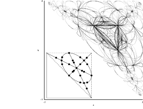
Figure 1: Polynomials $C_{N}$ in the $(a,\,b)$ parameter plane (upper right corner).

Let us display these various algebraic curves $\,C_{N}^{ij}$ in the $(a,\,\,b)$-parameter plane. One sees, on Figure 1 (upper right corner), that this accumulation of curves looks, a little bit, like a (discrete) “foliation” of the $(a,\,\,b)$-plane in curves similar to a linear pencil of algebraic curves [28], the “base points” of this linear pencil being, in fact, singular points of these $\,C_{N}$’s (see Appendix A) of lower complexity and sometimes, $(a,\,\,b)$ points for which the mapping becomes integrable.

On these algebraic curves $\,C_{N}^{ij}\,=\,0$ $(N=2,4,6,\cdots)$, the complexity is given by the inverse of the smallest root of:

$$1-2t+t^{N+2}\,=\,\,0$$ (23)

As $N$ increases, the complexity reads $\lambda=1.8392,1.9659,$ $1.9919,\cdots$ One recovers a family of complexities (depending on $\,N$) already seen for the Noetherian mappings [27] of the previous section and, even, for the mapping (1) for $\,\epsilon\,=\,1/N$ (see [18]). Actually, one finds a shift of $\,+1$ between (12) and (23).

In contrast with the situation encountered with the Noetherian mappings of the previous section (3.2) (see also [27]), the complexity reduction conditions are now involved families of polynomials (exponential degree growth in the $(a,\,b)$ parameters i.e. $\delta>1$), instead of the previous extremely simple, and separated conditions [27] in the $\,a$, $\,b$, $\,c$ variables ($a\,=\,(N-1)/N$, …).

Recalling the complexity reduction scheme described in section (3.2) for mapping (7), we saw further complexity reductions on the intersections of two complexity reduction conditions $\,a=\,(M-1)/M$ and $\,b\,=\,(N-1)/N$ ($M\,$ and $N\,$ positive integers) and $\,c\,=\,2-a-b\,$, namely families of complexities depending on the two integers $N\,$ and $\,M$ associated [27] with polynomials $\,1-2\,t+{t}^{M+1}+{t}^{N+1}-{t}^{M+N}$.

By analogy, it is natural to see if a similar complexity reduction scheme also occurs for mapping (16), by calculating the degree growth complexity when the parameters $a$, and $b$, are restricted to the intersection of two conditions $\,C_{N}^{ij}\,=\,0$. Actually, we have considered the intersection of $\,C_{2}^{31}\,=\,0\,$ and $\,C_{4}^{22}\,=\,0$, that we will denote symbolically $\,C_{2}^{31}\cap C_{4}^{22}$, as well as the intersection $\,C_{2}^{13}\cap C_{4}^{31}$. We obtained the following generating function in agreement with the successive degrees (up to $t^{9}$) in the corresponding iteration:

$$G_{C_{2}^{13}\cap C_{4}^{31}}\,=\,\,1+2\,t+4\,{t}^{2}+7\,{t}^{3}+13\,{t}^{4}+24\,{t}^{5}+43\,{t}^{6}+77\,{t}^{7}$$

$$\qquad\quad\quad+138\,{t}^{8}+247\,{t}^{9}\,+\cdots\,=\,\,{\frac{1-{t}^{3}}{1-2\,t+{t}^{4}+{t}^{6}-{t}^{8}}}$$ (24)

Keeping in mind the shift of $\,+1$ between (12) and (23), one might expect a formula like (13) for an intersection $\,C_{M}^{13}\cap C_{N}^{31}$ (or $\,C_{M}^{31}\cap C_{N}^{22}$)

$$Q_{M,N}\,=\,\,\,\,1\,-2\,t\,+{t}^{M+2}\,+{t}^{N+2}\,-{t}^{M+N+2}$$ (25)

This is actually the case with the previous example (4.1) where one has $\,M\,=2$ and $\,N\,=\,4$. Another example, also in agreement with (25), corresponds to the intersection $\,C_{4}^{31}\cap C_{6}^{13}$ for which one gets a rational degree generating function with denominator $1-2\,t+{t}^{6}+{t}^{8}-{t}^{12}$.

Note that such formula seems to remain valid even when $\,M\,=\,N$. For instance, for $C_{4}^{13}\cap C_{4}^{31}$ the denominator of the generating function reads $\,1-2\,t+2\,{t}^{6}-{t}^{10}$, and for $C_{6}^{13}\cap C_{6}^{31}$ the denominator reads $\,1-2\,t+2\,{t}^{8}-{t}^{14}$, in agreement with (25) for $\,M\,=\,N\,=\,6$.

One sees that one has exactly the same complexity reduction scheme, and the same family of complexity, as the one depicted in Section (3.2) for [27].

However, one does see a difference with the intersection of three conditions. For mapping (7), we saw [27] that the intersection of three conditions $\,a=\,(N-1)/N$, $\,b=\,(M-1)/M$, $\,c\,=2-(a+b)=\,P/(P+1)$, yields systematically integrable mappings. Here the $(a,\,b)$ points corresponding to intersection of three conditions $\,C_{N}^{ij}\,=\,0$ when they exist, may still yield an exponential growth of the calculations of lower complexity:

$$G_{C_{6}^{13}\cap C_{6}^{31}\cap C_{8}^{22}}\,=\,\,1+2\,t+4\,{t}^{2}+8\,{t}^{3}+14\,{t}^{4}+24\,{t}^{5}+40\,{t}^{6}+66\,{t}^{7}$$

$$\qquad\quad\,+108\,{t}^{8}\,+\cdots\,\,=\,\,{\frac{1+{t}^{3}}{\left(1-t\right)\left(1-t-{t}^{2}\right)}}\,=\,\,{\frac{1+{t}^{3}}{1-2\,t+{t}^{3}}}$$ (26)

We have a similar result for the intersection of the three curves $\,C_{2}^{31}\cap C_{6}^{31}\cap C_{10}^{31}$ with a denominator reading $\,1-2\,t+{t}^{4}$.

One should remark, in contrast with most of the degree growth rate calculations we have performed for so many birational transformations [14], that one can hardly find rational values for the two parameters $\,a$ and $\,b$, lying on the various $\,C_{N}^{ij}$’s we have just considered, (and of course it is even harder for intersections of such algebraic curves), such that one would deal with iterations of birational transformations with integer coefficients, and factorization of polynomials with integer coefficients. Such $\,(a,\,b)$ points on $\,C_{N}^{ij}$ algebraic curves or intersections of such curves, are algebraic numbers. The degrees of the successive iterates should correspond to factorizations performed in some field extension corresponding to these algebraic numbers and curves. In practice, results and series like the ones displayed above ((23), …, (4.1)), cannot be obtained this way. To achieve these factorizations, we have introduced a “floating” factorization method that is described in Appendix B.

4.2 Degree growth complexity versus topological entropy

The topological entropy is related to the growth rate of the number of fixed points of $\,K^{N}$ (see [12]). The counting of the number of primitive cycles of order $\,N$, for the generic case $[4,1,2,3,6,9,18,30,\cdots\,\,]$ gives a rational dynamical zeta function [18]

$$\zeta_{g}(t)\,=\,\,\,{{1}\over{\left(1-2\,t\right)\left(1-t\right)^{2}}}$$ (27)

which is related to the homogeneous degree generating function $G(K)$ by the identity:

$${\frac{t}{\zeta_{g}}}\cdot{{d}\over{dt}}\zeta_{g}\,\,=\,\,\,\,2\,G(K)(t)\,+\,\,{\frac{2\,t}{1-t}}\,\,=\,\,\,\,{\frac{2\,t}{1-2\,t}}+\,\,{\frac{2\,t}{1-t}}$$ (28)

Restricted to the curve of complexity reduction $\,C_{2}^{22}(a,\,b)\,=\,0$, the primitive fixed points become $[4,1,2,2,4,5,10,15,26,42,\cdots\,\,]$ giving the rational dynamical zeta function:

$$\zeta(t)\,=\,\,{\frac{1}{\left(1-2\,t+{t}^{4}\right)\left(1-t\right)^{2}}}$$ (29)

Again, note that this dynamical zeta function is related to the homogeneous degree generating function $G(K)$ (corresponding to $\,C_{2}^{22}(a,\,b)\,=\,0$), by the identity:

$${\frac{t}{\zeta}}\cdot{{d}\over{dt}}\zeta\,\,=\,\,\,\,2\,G(K)(t)\,+\,\,{\frac{2\,t}{1-t}}\,\,\,=\,\,\,{{2\,t\cdot(1-2\,t^{3})}\over{1-2\,t+{t}^{4}}}\,+\,\,{\frac{2\,t}{1-t}}$$ (30)

We thus see, with these two examples (and similarly to the results obtained for the birational transformations [12, 18] as well as the Noetherian mappings [27]), an identification between the growth rate of the number of fixed points of $\,K^{N}$, and the growth rate of the degree of the iteration (previously studied (16)), or equivalently, the growth rate of the Arnold complexity.

Relations (28) and (30) are in agreement with a Lefschetz formula:

$$\nu_{N}\,=\,\,\,d_{N}(K)\,+\,\,d_{N}(K^{-1})\,+\,\,1\,+\,\,1$$ (31)

where $\,\nu_{N}$ denotes the number of fixed points of $\,K$ or $\,K^{-1}$, $\,d_{N}(K)$ denotes the degree of $\,K^{N}$, $\,d_{N}(K^{-1})$ the degree $\,K^{-N}$. This formula (31) means that the number of fixed points is the sum of four “dynamical degrees [30]” $\,\delta_{0}\,+\,\delta_{1}\,+\,\delta_{2}\,+\,\delta_{3}$. Dynamical degree $\,\delta_{0}$ is always equal to $\,+1$, $\,\delta_{3}$ is the topological degree (number of preimages: $\,\delta_{3}$ is equal to $\,+1$ for a birational mapping), $\,\delta_{1}$ is the first dynamical degree (corresponding to $\,d_{N}(K)$) and $\,\delta_{2}$ is the second dynamical degree (corresponding to $\,d_{N}(K^{-1})$).

Remark 1: Most of the physicists will certainly take for granted that the degree growth rate corresponding to the iteration of $\,K$ and its inverse $\,K^{-1}$ identify: $\,d_{N}(K)\simeq\,\lambda(K)^{N},$ $\,d_{N}(K^{-1})\simeq\,\lambda(K^{-1})^{N}$, with $\,\lambda(K)\,=\,\lambda(K^{-1})$. This is actually the case for all the birational transformations we have studied [18]. In the specific examples of this paper, this is, in the involutive case $\,\xi\,=\,a+b+c-1\,=\,1$, a straight consequence of the fact that $\,K$ and $\,K^{-1}$ are conjugated. More generally, this fact can be proved for all birational transformations in $\,CP_{2}$, but certainly not for birational transformations in $\,CP_{n}$, $\,n\,\geq 3$ (for instance birational transformations generated by products of more than two involutions, or “Noetherian” mappings products of many collineations and Hadamard involutions [27], such that $\,K$ and $\,K^{-1}$ are not conjugated). Appendix C provides a simple example of bi-polynomial transformation in $CP_{3}$ such that $\,\lambda(K)\,\neq\,\lambda(K^{-1})$.

Remark 2: The very definition of the dynamical zeta function on $\,C_{0}(a,\,b)\,=\,0$ is a bit subtle, and problematic, since the number of fixed points for $\,K^{2}$ (and thus $\,K^{2N}$) is actually infinite (one has a whole curve (34) of fixed points of order two). Apparently, in that case where an infinite number of fixed points of order two exist, one does not seem, beyond these cycles of order two, to have primitive cycles of even order. Introducing the dynamical zeta function as usual, from an infinite Weil product [18] on the cycles, and taking into account just the odd cycles, one obtains (more details are given in Appendix D) that this zeta function verifies a simple functional equation

$$\zeta(t^{2})\,=\,\,{{(1-2\,t)\cdot(1-t)^{2}}\over{(1+2\,t)\cdot(1+t)^{2}}}\cdot\zeta(t)^{2}$$ (32)

showing that, the complexity is still the generic $\,\lambda\,=\,2$ but, this time, with an expression which is not a rational function, but some “transcendental”expression. In order to have a Lefschetz formula (31) remaining valid, in such highly singled-out cases for dynamical zeta functions, one needs to modify the definition of the dynamical zeta function so that it is no longer deduced from an infinite Weil product [18] formula on the cycles. To be more specific, this must be performed using the so-called [31] “Intersection Theory” which is a (quite involved) theory introduced to cope with isolated points, as well as non-isolated points (curves …), introducing some well-suited (and subtle) concepts like the notion of multiplicity. All the associated counting of intersection numbers will, then, correspond to counting of finite integers (replacing the counting of cycles …). This is far beyond the scope of this very paper.

5 Preserved meromorphic two-forms in particular subspaces $(a,b)$

In Appendix E, we show that the degree growth (in the $(a,\,b)$ parameters) for the iterates of the three curves of the critical set (resp. exceptional locus) when the parameters are restricted to $b=a$, $b=2-2a$, $b=\,1-2a$, and $C_{0}(a,b)=0$, is polynomial ($\delta=1$). The iterates are found in closed expressions. Let us show that, in these cases, the mapping $K$ preserves simple meromorphic two-forms.

On the three lines $\,b=a$, $b=\,2\,-2a\,$, and $b=1-a/2$, one finds three preserved meromorphic two-forms reading respectively:

$${{du\cdot dv}\over{(u-1)\cdot(2\,(2a-1)(u+v^{2})\,+(5a-4)(1+u)\,v)}}\,=\,\,idem(u^{\prime},\,v^{\prime})$$

$${{du\cdot dv}\over{(v-1)\cdot((5a-4)(1+v)u+2(2a-1)(v+u^{2}))}}\,=\,\,idem(u^{\prime},\,v^{\prime})$$

$${{du\cdot dv}\over{(v-u)\cdot(4(a-1)(1+uv)+(5a-2)(v+u))}}\,=\,\,idem(u^{\prime},\,v^{\prime})$$ (33)

The second, and third, two-forms are obtained from the first one in (5) by respectively $(u,v)\rightarrow(v,u)$ for $b=2-2a$, and by $(u,v)\rightarrow(u/v,1/v)$ with $a\rightarrow 1-a/2$, for $b=1-a/2$. For the quadratic condition $C_{0}(a,b)=0$, the mapping preserves the following two-form, up to a minus sign:

$${{du\cdot dv}\over{\rho(u,\,v)}}\,=\,\,\,-\,{{du^{\prime}\cdot dv^{\prime}}\over{\rho(u^{\prime},\,v^{\prime})}},\quad\quad\quad\quad\quad\hbox{where :}$$

$$\rho(u,\,v)\,=\,\,\,\,(b-a)(a^{2}+b^{2}+3ab)\,(1+u^{2})\,v$$

$$\quad\quad\quad-(2b+a)(a^{2}-b^{2}-ab)\,(1+v^{2})\,u$$ (34)

$$\quad\,\,\quad-(b+2a)(a^{2}-b^{2}+ab)\,(u^{2}+v^{2})+2(b-a)(2a+b)(a+2b)\,uv$$

Note that $\,\rho(u,\,v)\,=\,0$ is an elliptic curve.

Considering the 25 points $(a,\,b)$, listed in Appendix F, for which the mapping is integrable, one can see that they all belong to the codimension-one subvarieties of the $(a,\,b)$ plane, where preserved meromorphic two-forms are found, i.e. the curve $C_{0}(a,b)=0$ and/or the lines $b=a$, $b=2-2a$, $b=1-a/2$ (see Figure 1, lower left corner).

Furthermore, when these codimension-one subvarieties intersect, the deduced $(a,\,b)$ points correspond to integrability of the mapping. The algebraic invariants corresponding to these integrability cases, can easily be deduced from the fact that, at the intersection of two curves among $\,C_{0}(a,b)=0$, and the lines $b=a$, $b=2-2a$, $b=1-a/2$, one necessarily has two simple two-forms preserved (up to a sign). Performing the ratio of two such two-forms one immediately gets algebraic invariants of the integrable mapping. See Appendix F for examples of algebraic invariants deduced, for integrable points $(a,\,b)$, from ratio of two preserved two-forms.

Remark: One may have the feeling that the exact results on preserved meromorphic two-forms, or in the previous sections on complexity reduction for (16), are consequences of the fact that we restricted ourselves to $\,\xi\,=\,a+b+c-1\,=\,1$, the condition for collineation $\,C$ to be involutive (yielding $\,K$ and $\,K^{-1}$ to be conjugate). This is not the case. We give in Appendix G miscellaneous examples of exact results valid when this involutive condition on $\,C$ is not verified ($\,\xi\,=\,a+b+c-1\,\neq\,1$).

It is tempting, after such an accumulation of preserved two-forms, to see the previous results (5), (34) as a restriction to these codimension-one subvarieties in the ($a,\,b)$-plane, of a general (conformally preserved) meromorphic two-form valid in the whole $(a,\,b)$-plane. In view of the expressions of the two-forms for the three lines on one side, and the expression associated with the elliptic curve (5) on the other side, one could expect, at first sight, this meromorphic two-form to be quite involved. Using a ”brute force” method we have tried to seek, systematically, for meromorphic two-forms $\,d\mu(u,\,v)=du\cdot dv\,/\rho(u,\,v)$, with an algebraic (polynomial) covariant $\,\rho(u,\,v)$ in the form:

$$\rho(u,\,v)\,=\,\,\,\,\sum_{i=0}^{n_{1}}\sum_{j=0}^{n_{2}}c_{ij}\,u^{i}\,v^{j}.$$ (35)

The existence of such a polynomial covariant curve is ruled out up to $n_{1}=n_{2}=18$. Formal calculations seem hopeless here, in particular if the final result is a non existence of such an algebraic covariant of (16) for generic $a,\,b$. One needs to develop another approach that might be also valid to prove a “no go” result like the non existence of an algebraic covariant $\,\rho(u,\,v)$, and beyond, the non existence of a “transcendental” covariant $\,\rho(u,\,v)$, corresponding to some analytic but not algebraic curve.

6 Orbit of the critical set: algebraic curves versus chaotic sets

When a preserved (resp. conformally preserved) meromorphic two-form $du.dv/\rho(u,\,v)$ exists, one has the following fundamental relation (3) between the algebraic expression $\rho(u,\,v)$ and the Jacobian of transformation $\,K$:

$$\rho\left(K(u,\,v)\right)\,\,=\,\,\,\xi\cdot J(u,\,v)\cdot\rho(u,\,v)$$ (36)

where $\,\xi$ is a constant. When $\,\xi\,=\,+1$ the two-form is preserved. When there exists an integer $\,M$, such that $\,\xi^{M}\,=\,1$, the transformation $\,K^{M}$, instead of $\,K$, preserves a two-form. When $\,\xi\,\neq\,+1$ (for any $M$, $\,\xi^{M}\,\neq\,+1\,$), it is just conformally preserved. Let us restrict the previous fundamental relation (36) to a point $(u,\,v)$ such that the Jacobian of transformation $\,K$ vanishes, $\,J(u,\,v)\,=\,0$. The fundamental relation (36) necessarily yields for such a point:

$$\rho\left(K(u,\,v)\right)\,\,=\,\,\,0$$ (37)

For birational transformations, the images of the curves $\,J(u,\,v)\,=\,0$ are not curves but blow down into set of points. For mapping (16), the vanishing condition $\,J(u,\,v)\,=\,0$ splits into three curves $u=0$,$\,v=0$ and $u=-av/(v(a-1)+a)$. The image of these three curves blow down into three points $(u^{(1)},\,v^{(1)})$, $(u^{(2)},\,v^{(2)})$ and $(u^{(3)},\,v^{(3)})$. Being covariant, $\rho(u,\,v)$ not only vanishes at these points (i.e. $\rho(u^{(i)},\,v^{(i)})=0$ for $i=1,\,2,\,3$), but also on their orbits:

$$\rho\left(K^{N}(u^{(i)},\,v^{(i)})\right)\,\,=\,\,\,0,\qquad\quad\quad N\,=1,\,2,\,\cdots,\,i=1,\,2,\,3$$ (38)

One can thus construct a (generically) infinite set of points on $\rho(u,\,v)=0$, as orbits of such “singled-out” points $(u^{(i)},\,v^{(i)})$ and visualize them, whatever (the accumulation of) this set of points is (algebraic curves, transcendental analytical curves, chaotic set of points, …).

Before visualizing some orbits, let us underline that (38) means that the iterates of the critical set, also called post-critical set, actually cancel $\rho\left(u,\,v\right)$. These iterates are known in closed forms for some subspaces. For instance, on the line $b=a$, the iterates are given in Appendix E in terms of Chebyshev polynomials. At these iterates $\left(u^{(i)}_{N},\,v^{(i)}_{N}\right)$, with closed expressions, one has $\rho\left(u^{(i)}_{N},\,v^{(i)}_{N}\right)=0$.

The meromorphic two-forms found in Section (5) (see (5)), actually correspond to situations such that the post-critical set (resp. the orbit of the exceptional locus) has $\,\delta\,=\,1$, closed expressions being available to describe all these points (Chebyshev polynomials, …). The generic exponential growth (in the parameters) of the $\left(u^{(i)}_{N},\,v^{(i)}_{N}\right)$ (namely $\,\delta\sim 2$), certainly excludes (even very involved) algebraic expressions (35) for $\rho(u,\,v)$, but it may not exclude transcendental analytical curves (like the transcendental curves (31) in paragraph 7 of [27], or the transcendental curves (20) in [32], which are orbits of a birational transformation exhibiting some “transcendental” integrability [27, 33].)

6.1 Visualization of post-critical sets

Figure 2: Orbit of the critical set for $(a,\,b)\,=\,(0,\,1.9)$

Figure 3: Orbit of the critical set for $(a,\,b)\,=\,(-.2,\,.7)$

Let us visualize a few post-critical sets. In the cases where a meromorphic two-form is actually preserved (see (5)), one easily verifies that the orbit of $(u^{(1)},\,v^{(1)})\,=\,(b/a,\,\,(1-a-b)/a)$, actually yields the (whole) covariant condition $\,\rho(u,\,v)\,=\,0$ corresponding to the divisor of a meromorphic two-form when such a meromorphic two-form has been found. Of course if one performs iterations of other points (even very close) than the singled out points as $\,(b/a,\,\,(1-a-b)/a)\,$, one will not get such algebraic covariant curve $\,\rho(u,\,v)\,=\,0$, but more involved orbits. In contrast for parameters $(a,\,b)$ for which no meromorphic two-form was found, we see a drastically different situation, shown in Figure 2, corresponding to the orbit of $\,(b/a,\,\,(1-a-b)/a)$ (image by transformation $\,K$ of one of the vanishing conditions for the Jacobian) for $(a,\,b)\,=\,(0,\,1.9)$.

This post-critical set (Figure 2) looks very much like a set of curves, a “foliation” of the $\,(u,\,v)$-plane. Figure 3 shows the post-critical set corresponding to the case $(a,\,b)\,=\,(-.2,\,.7)$. With these two orbits it is quite clear that this set of points cannot be a simple algebraic curve $\,\rho(u,\,v)\,=\,0$.

At this step the “true” nature of this set of points is almost a “metaphysical” question: is it a transcendental analytical curve infinitely winding, is it a chaotic fractal-like set … ? In particular when one takes a larger frame for plotting the orbit, the set of points becomes more fuzzy, and it becomes more and more difficult, to see if these points are organized in curves, like Figure 2 which suggests an (infinite …) accumulation of curves. We have encountered many times such a situation (see paragraph 5.1 and Figures 13 and 14 in [11]). A way to cope with the fuzzy appearance of the orbit when the points go to infinity, is to perform a change of variables (see paragraph 5 in [11]): $(u,\,v)$ $\,\rightarrow\,$$(1/u,\,1/v)$. Again one has the impression to see some kind of “foliation of curves” for the previously fuzzy points, but the points that were seen in Figure 2 as organized like a “foliation” of curves, have now (in some kind of “push-pull game”) become fuzzy sets. One way to avoid this “push-pull” problem, and thus, “see the global picture” amounts to performing our plots in the variables $\,u_{c}\,=\,u/(1+u+u^{2})$ and $\,v_{c}\,=\,v/(1+v+v^{2})$. These variables are such that any orbit of real points will be in the box $\,[-1,\,1/3]\times[-1,\,1/3]$. This trick “compactifies”automatically our orbits.

Figure 4: The orbit of the critical set in the “compact” variables $\,u_{c}$ and $\,v_{c}$, for $\,(a,\,b)\,=\,(-.2,\,.72)$

Figure 5: The orbit of the critical set in the “compact” variables $\,u_{c}$ and $\,v_{c}$, for $\,(a,\,b)\,=\,(-.2,\,.999999999)$

Let us give two examples of such “compactified” images of two orbits of $\,(b/a,\,\,(1-a-b)/a)$ (image by transformation $\,K$ of one of the vanishing conditions for the Jacobian). For $\,(a,\,b)\,=\,(-.2,\,.72)$ one gets Figure 4, and for $\,(a,\,b)\,=\,(-.2,\,.999999999)$ one gets Figure 5.

In the situation where preserved meromorphic two-forms exist, one sees that, even a very small deviation from the $\,(b/a,\,\,(1-a-b)/a)$ point (associated with the post-critical set), yields orbits that look quite different from the algebraic covariant curve $\,\rho(u,\,v)\,=\,0$. In contrast with this situation, we see, in the previous cases where no preserved meromorphic two-forms exist, that a slight modification of the $\,(b/a,\,\,(1-a-b)/a)$ point (associated with the post-critical set) yields orbits which are extremely similar to the post-critical set of Figures (3) or (4), or (5). These orbits are “similar”, but not converging towards this post critical set. They are, roughly speaking, “parallel” to this post critical set. Therefore the orbit of the critical set may be seen as a chaotic set, but it is a non attracting chaotic set in contrast with the well-known strange attractors of Hénon bi-polynomial mappings [34, 35].

6.2 From preserved meromorphic two-forms and post-critical sets back to fixed points

Denoting $(u^{\prime},\,v^{\prime})$, $(u^{\prime\prime},\,v^{\prime\prime})$, …, $\,(u^{(n)},\,v^{(n)})$, the images of a point $(u,\,v)$, by transformations $\,K$, $\,K^{2}$, …, $\,K^{n}$, the preservation of a two-form yields ($J[K^{n}](u,\,v)$ being the Jacobian of $\,K^{n}$):

$${{du\cdot dv}\over{\rho(u,\,v)}}\,\,=\,\,\,{{du^{\prime}\cdot dv^{\prime}}\over{\rho(u^{\prime},\,v^{\prime})}}\,\,=\,\,\,\cdots\,\,=\,\,\,{{du^{(n)}\cdot dv^{(n)}}\over{\rho(u^{(n)},\,v^{(n)})}}$$

$$J[K^{n}](u,\,v)\,\,=\,\,\,{{\rho(u^{(n)},\,v^{(n)})}\over{\rho(u,\,v)}}\,\,=\,\,\,{{\rho(K^{n}(u,\,v))}\over{\rho(u,\,v)}}$$ (39)

From the previous relation, it is tempting to deduce (a little bit too quickly …) that the Jacobian of $\,K^{n}$ is equal to +1 when evaluated at the fixed point $(u_{f},v_{f})$ of $\,K^{n}$:

$$J[K^{n}](u_{f},\,v_{f})\,=\,\,\,{{\rho(K^{n}(u_{f},\,v_{f}))}\over{\rho(u_{f},\,v_{f})}}\,=\,\,+1$$ (40)

We actually found such strong results for (1), and for many other birational transformations (when, for instance, we evaluated precisely the number of $n$-cycles, to get the dynamical zeta function [18]), for which a meromorphic two-form was actually preserved. In fact, even when a meromorphic two-form is preserved, relation (40) (namely the Jacobian of $\,K^{n}$ evaluated at a fixed point of $\,K^{n}$, is equal to +1), may be ruled out when the fixed points of $\,K^{n}$ correspond to divisors of the two-form. If $\,\rho(u,\,v)$, corresponding to a preserved meromorphic two-form, is a rational expression $\,\rho(u,\,v)\,=\,P(u,\,v)/Q(u,\,v)$ ($P(u,\,v)$ and $\,Q(u,\,v)$ are polynomials), the Jacobian of $\,K^{n}$, evaluated at a fixed point $\,(u_{f},\,v_{f})$ of $\,K^{n}$, can actually be different from $\,+1$, if $P(u_{f},\,v_{f})\,=\,\,0$, or $\,Q(u_{f},\,v_{f})\,=\,\,0$. Such “non-standard” fixed points of $\,K^{n}$ are such that $\,\rho(u_{f},\,v_{f})\,=\,\,0$ (resp. $\,\rho(u_{f},\,v_{f})\,=\,\,\infty$), and of course, since $\rho(u,\,v)$ is typically a covariant of $\,K$ (see (36)), such that $\rho(u,\,v)$, evaluated at all their successive images by $\,K^{N}$ (for any $N$ integer), vanishes (resp. is infinite):

$$J[K^{n}](u_{f},\,v_{f})\,\neq\,+1,\quad\Rightarrow\quad\rho(K^{N}(u_{f},\,v_{f}))\,=\,\,0\,\quad\hbox{(resp. $\,\infty$) }$$ (41)

Performing orbits of such “non-standard” fixed points could thus be seen as an alternative way of visualization of $\rho(u,\,v)$ (whatever its “nature” is: polynomial, rational expression, analytic expression, … ), this alternative way being extremely similar to the one previously described, associated with the visualization of post-critical sets. Finding by formal calculations a very large accumulation of such “non-standard” fixed points is not sufficient to prove the non-existence of meromorphic two-forms: one needs to be sure that this accumulation of points cannot be localized on some unknown highly involved algebraic curve. It is well known that proving “no-go” theorems is often much harder than proving theorems that simply require to exhibit a structure. However, as far as this difficulty to prove a non-existence is concerned, it can be seen as highly positive and effective, as far as simple “down-to-earth” visualization methods are concerned. In contrast with the unique post-critical set, we can consider orbits of a large (infinite) number of such “non-standard” fixed points of $\,K^{n}$. The relation between the post-critical set and such “non-standard” sets, is a very interesting one that will be studied elsewhere.

Let us just consider the birational transformation (16) for $(a,\,b)=\,(-1/5,\,1/2)$ (where no meromorphic two-form has been found). The primitive fixed points (cycles) and the value of the Jacobian of $\,K^{n}$ at the corresponding fixed points, that we will denote $\,J$, are given  in Table 1.

$n$ 1 2 3 4 5 6 7 8 fix$(K^{n})$ 4 1 2 3 6 9 18 30 $J=1$ 0 1 0 1 0 3 0 6 $|J|=1$ 2 0 2 2 4 4 6 8 $J\neq 1$ 2 0 0 0 2 2 4 4 $|J|\neq 1$ 0 0 0 0 0 0 8 12

Table 1: Counting of primitive cycles for $a=-1/5,\,b=1/2$. $\,J$ denotes $J[K^{n}](u_{f},\,v_{f})$. The number of cycles are in agreement with the Weil product expansion of the known (see (27)) exact expression of the dynamical zeta function:

$$\zeta(t)\,\,=\,\,{{1}\over{\left(1-2\,t\right)\left(1-t\right)^{2}}}\,\,=\,\,{\frac{1}{\left(1-t\right)^{4}\left(1-{t}^{2}\right)\left(1-{t}^{3}\right)^{2}\left(1-{t}^{4}\right)^{3}}}\,\times$$

$$\quad\quad\quad\quad\times\,{{1}\over{\left(1-{t}^{5}\right)^{6}\left(1-{t}^{6}\right)^{9}\left(1-{t}^{7}\right)^{18}\left(1-{t}^{8}\right)^{30}\cdots}}$$ (42)

To some extent, the situations where $\,J\,=\,-1$, or where $\,J$ is an $N$-th root of unity, can be “recycled” into a $\,J\,=\,1$ situation, replacing $\,K^{n}$ by $\,K^{2\,n}$ or $\,K^{N\,n}$. However, we see on Table 1, the beginning of a “proliferation” of “non-standard”points that cannot be reduced to $\,J\,=\,-1$ or $\,J^{N}\,=1$, strongly suggesting the non-existence of a meromorphic two-form. These enumerations have to be compared with the ones corresponding to $(a,\,b)=\,(1/5,\,1/5)$, for which a meromorphic two-form is actually preserved. We still have the same sequence $\,4,\,1,\,2,\,3,\,6,$$\,9,\,18,\,30,\cdots$ of $\,n$-cycles, associated to the same dynamical zeta function (6.2), however (except for the fixed points of order one), all the fixed points of order $\,n\,\geq 2$ are such that $\,J\,=\,1$ .

Along this line, let us consider mapping $K$ on curve $C_{2}^{22}(a,b)=0$, where, despite the complexity reduction, no meromorphic two-form has been found. The calculations are performed for the (generic) values $a=12/13,\,b=-3/13$ (the number of non generic $(a,b)$ on $C_{2}^{22}(a,b)$ is finite) and are given in Table 2.

$n$ 1 2 3 4 5 6 7 8 9 10 fix$(K^{n})$ 4 1 2 2 4 5 10 15 26 42 $J=1$ 0 1 0 0 0 1 0 3 0 6 $|J|=1$ 2 0 0 0 2 2 0 2 4 2 $J\neq 1$ 2 0 2 2 2 2 6 6 10 14 $|J|\neq 1$ 0 0 0 0 0 0 4 4 12 20

Table 2: Counting of primitive cycles for $(a,b)$ such that $C_{2}^{22}(a,b)=0$. $\,J$ denotes $J[K^{n}](u_{f},\,v_{f})$.

The number of $\,n$-cycles are of course, in agreement with the Weil product decomposition of the exact dynamical zeta function (29). We note the same proliferation of “non-standard” fixed points of order $\,n$, in agreement with the non-existence of a preserved meromorphic two-form. This last result confirms what we saw several times, namely the disconnection between the existence (or non-existence) of a preserved meromorphic two-form and (topological) complexity reduction for a mapping.

6.3 Pull-back of the critical set : “ante-critical sets” versus post-critical sets

As far as visualization methods are concerned physicists, “fortunately”, perform iterations without being conscious of the potential dangers: birational transformations have singularities and they may proliferate when performing iterations. More precisely, the critical set (vanishing conditions of the Jacobian) is a set of curves, whose images, by transformation $\,\,K$, yield points and not curves (blow-down). In contrast, the images by transformation $\,\,K^{-1}\,$ (resp. $\,\,K^{-N}$) of these curves of the critical set (denoted in the following CS) give curves: we do not have any blow-down with $\,\,K^{-1}$ (resp. $\,\,K^{-N}$). This infinite set of curves obtained by iterating the critical set by $\,\,K^{-1}$, is such that, for some finite integer $\,N$, the image of these curves by $\,\,K^{N}$ will blow down into points, after a finite number $\,N$ of iterations. Let us call this set, for obvious reasons, “ante-critical set”. This “ante-critical set” is clearly a “dangerously singular” set of points for the iteration of $\,K$. It is also a quite interesting set from the singularity analysis viewpoint [1]. In particular, among these “dangerous points” associated with the infinite set of curves $\,\Gamma_{N}\,=\,K^{-N}(CS)$, some are singled-out (more “singular” …): the points corresponding to intersections of two (or more) such curves $\,\Gamma_{N}$’s. These singled-out points can, in fact, be obtained by some simple “duality” symmetries from the points of the post-critical set. Such “ante-critical sets”, and their associated consequences on the birational transformations $\,K$, clearly require some further analysis that will be performed elsewhere.

7 Lyapunov exponents and non-existence of meromorphic two-forms

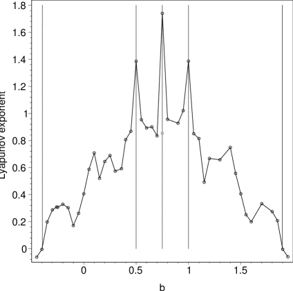
Figure 6: Lyapunov exponents as a function of parameter $\,b$, for $\,a\,=\,1/2$, the initial point being $\,(u,\,v)\,=\,\,(2,\,3)$.

Figure 7: Lyapunov exponents as a function of parameter $\,b$, for $\,a\,=\,1/2$, the initial point being the image of the critical set.

The previous simple visualization approach can be confirmed by some Lyapunov exponents analysis. Let us consider orbits of a given initial point (for instance $\,(u,\,v)\,=\,\,(2,\,3)$) under the iteration of birational transformation (16) for parameter $\,a$ fixed (for instance $\,a\,=\,1/2$), and for different values of the second parameter $\,b$, and let us calculate the corresponding Lyapunov exponent. One thus gets the Lyapunov exponent (of what we can call a “generic” orbit) as a function of parameter $\,b$. This simple analysis is an easy down-to-earth way to detect drastic complexity reductions, the complexity being not the topological complexity (like the topological entropy or the growth rate complexity) but a less universal (more probabilistic) complexity (like the metric entropy).

Figures (6), (7) show, quite clearly, non-zero and positive Lyapunov exponents, such results being apparently valid, not only for the Lyapunov exponent corresponding to our singled-out orbit, the post-critical set (see Figure (7)), but, also, for every orbit in the $(u,\,v)$-plane (see Figure (6)). With this scanning in the $\,b$ parameter we encounter several times the singled-out cases where preserved meromorphic two-forms exist ($a\,=b$, $\,C_{0}(a,\,b)\,=\,0$, …, see (5)), and we see that these specific points are singled-out on Figure (6). If instead of performing the orbit of an arbitrary point ($(u,\,v)\,=\,\,(2,\,3)$) one calculates the Lyapunov exponent corresponding to the post-critical set one finds similar results with a quite high volatility (a value of $\,b$ where the Lyapunov is a “local” maximum is quite close to a value where the Lyapunov is almost zero).

In order to better understand this volatility, we have performed specific Lyapunov exponents calculations restricted to the singled-out cases where preserved meromorphic two-forms exist ($a\,=b$, $\,C_{0}(a,\,b)\,=\,0$, …, see (5)). In such cases we recover the situation we had [12] with birational mapping (1), namely the Lyapunov exponents are zero (or negative on the attractive fixed points) for all the orbits we have calculated (the positive non-zero Lyapunov being possibly on some “evanescent” slim Cantor set [21, 22], see section (2), that we have not been able to visualize numerically) and the orbits always look like curves. It is clear that computer experiments like these, can hardly detect the slim and subtle Cantor sets corresponding to (wedge product) invariant measure described [21, 22] by Diller and Bedford in such situations, associated with the narrow regions where non-zero positive Lyapunov could be found: within such (extensive) computer experiments we find, “cum grano salis”, that the Lyapunov exponents are “generically” (as far as computer calculations are concerned …) zero.

With this subtlety in mind, our computer experiments show clearly non-zero positive Lyapunov exponents when there is no preserved meromorphic two-form and a total extinction of these Lyapunov exponents when such preserved meromorphic two-forms take place.

The occurrence of non zero positive Lyapunov exponents for hyperbolic systems, or dynamical systems with strange attractors is well-known: this is not the situation we describe here.

8 Conclusion

The birational transformations in $\,CP_{2}$, introduced in section (4), which generically do not preserve any meromorphic two-form, are extremely similar to other birational transformations we previously studied [27], which do preserve meromorphic two-forms. We note that these two sets of birational transformations exhibit totally similar results as far as topological complexity is concerned (degree growth complexity, Arnold complexity and topological entropy), but drastically different numerical results as far as a more “probabilistic” (ergodic) approach of dynamical systems is concerned (Lyapunov exponents). With these examples we see that the existence, or non-existence, of a preserved meromorphic two-form explains most of the (disturbing) apparent discrepancy, we saw, numerically, between the topological and probabilistic approaches of such dynamical systems.

The situation is as follows. When these birational mappings preserve a mero-morphic two-form (conservative reversible case) the (preliminary) results of Diller and Bedford [21, 22] on mapping (1) give a strong indication (at least in the region of the parameter $\,\epsilon\,<\,0$ ) that the regions where the chaos is concentrated, namely where the Lyapunov exponents are non-zero and positive, are quite evanescent, corresponding to an extremely slim Cantor set associated with an invariant measure given by some wedge product. This nice situation from a differential viewpoint (existence of a preserved two-form), is the unpleasant one from the computer experiments viewpoint: it is extremely hard to see the “chaos” (homoclinic tangles, Smale’s horseshoe, …) from the analysis (visualization of the orbits, Lyapunov exponents calculations, …) of even very large sets of real orbits.

On the contrary, when the birational mappings do not preserve a meromorphic two-form, the regions where the Lyapunov exponents are non-zero, and positive, can, then, clearly be seen on computer experiments.

In conclusion, the existence, or non-existence, of preserved meromorphic two-forms has (curiously) no impact on the topological complexity of the mappings, but drastic consequences on the numerical appreciation of the “probabilistic” (ergodic) complexity.

The introduction of the post-critical set, namely the orbit of the points obtained by the blow-down of the curves corresponding to the vanishing conditions of the Jacobian of the birational transformation, thus emerges as a fundamental concept, and tool (of topological and algebraic nature) to understand the probabilistic (and especially numerical) subtleties of the dynamics of such reversible [8, 9] mappings.

Acknowledgments We thank C. Favre for extremely useful comments on analytically stable birational transformations, exceptional locus and indeterminacy locus, and its cohomology of curves approach of growth rate complexity. We thank J-C. Anglès d’Auriac and E. Bedford for many discussions on birational transformations. We also thank J-P. Marco for interesting discussions on invariant measures. (S. B) and (S. H) acknowledge partial support from PNR3.

9 Appendix A: Algebraic geometry: singularities of curves as candidates for complexity reduction

The conditions of reduced complexity give the points $(a,b)$ that belong to the algebraic curves $C_{N}$. These algebraic curves are such that one has a reduced complexity for generic point $(a,b)$ on the curve. However, singularities of these algebraic curves (from a purely algebraic geometry viewpoint: local branches, …) can actually be seen to correspond to points $(a,\,b)$ in the parameter plane yielding lower complexities for the birational transformation $\,K$.

On each curve $C_{N}$, the spectrum of complexity at the singularities is given by

$$1-2t+t^{p+2}\,=\,\,\,\,0,\qquad\quad p\,=\,0,\,1,\,\cdots,\,N/2-2$$ (43)

For example, a generic point on the curve $C_{8}^{22}$, has the complexity growth $\lambda=1.9980$. The singularities of this curve are non generic points and have complexity growth $\lambda\simeq 1,1.6180,1.8392$ given by (43) for $N=8$. The next curve $C_{10}^{22}$ with $\lambda\simeq 1.9995$, will inherit the last three values and adds (since $p$ goes now to 3) $\lambda\simeq 1.9275$. Note that for a given curve $C_{N}$, the largest value of complexity growth reached by its singularities is given by $1-2t+t^{N/2}$.

Let us give the generating functions of the degrees $\,d_{N}$, and genus $\,g_{N}$, of the successive $C_{N}(a,\,b)=0$ algebraic curves. Let us also introduce the generating function for $\,S_{N}$, the number of singularities of the algebraic curves $C_{N}$:

$$d_{C}(t)=\sum_{n=1}^{\infty}d_{2\,n}\cdot t^{2\,n},\quad g_{C}(t)=\sum_{n=1}^{\infty}g_{2\,n}\cdot t^{2\,n},\quad s_{C}(t)=\sum_{n=1}^{\infty}S_{2\,n}\cdot t^{2\,n}$$

They read respectively (for $C_{N}^{22}$ up to $N=12$):

$$d_{C}(t)\,=\,\,\,\,\,\,2\,t^{2}\,+\,6\,t^{4}\,+\,12\,t^{6}\,+\,26\,t^{8}\,+\,48\,t^{10}\,+\,\,98\,t^{12}\,+\,\cdots$$

$$g_{C}(t)\,=\,\,\,\,\,0\,t^{2}\,+5\,t^{4}\,+\,20\,t^{6}\,+\,73\,t^{8}\,+\,182\,t^{10}\,+\,\,491\,t^{12}\,+\,\cdots$$

$$s_{C}(t)\,=\,\,\,\,\,0\,t^{2}\,+5\,t^{4}\,+\,15\,t^{6}\,+\,31\,t^{8}\,+\,53\,t^{10}\,+\,\,113\,t^{12}\,+\,\cdots$$

The degrees $\,d_{N}$, the genus $\,g_{N}$, and the number of singularities $\,S_{N}$ clearly grow exponentially like $\,\lambda^{2n}$ with $\,\lambda\,<\,2$. We have no reason to believe that these three generating functions $\,d_{C}(t)$, $\,g_{C}(t)$ and $\,s_{C}(t)$, could be rational expressions. Similarly, their corresponding coefficients growth rates, $\,\lambda$, have no reason, at first sight, to be algebraic numbers.

A singularity of an algebraic curve is characterized by the coordinates of the singularities in homogeneous variables, the multiplicity $m$, the delta invariant $\delta$ and the number of local branches $r$. In general $m\geq r$ and $\delta\geq m(m-1)/2$. The equality holds for all the singular points of $C_{N}$, however, as $N$ increases, some points do not satisfy the equality. These points are $(a=0,b=1)$, $(a=1,b=0)$, $(a=1,b=1)$ and $(a=0,b=0)$, $(a=0,b=2)$, $(a=2,b=0)$.

10 Appendix B: Computing complexity growth of points known in their floating forms

Let us show how to compute the complexity growth of generic (algebraic) points on algebraic curves, and how to compute the complexity growth of points known in their floating forms.

To compute the complexity growth for the parameters $(a,b)$ belonging to a whole curve, e.g. $C(a,b)=0$, we fix $v$ (for easy iteration), and we iterate up to order $N$. We eliminate $b$ between the numerator of $u_{N}-X$ and the curve $C(a,b)=0$. We can obtain factorizable polynomials $P_{1}\cdot P_{2}\cdots$ One counts the degree of $u$ in the polynomials depending on $X$, and discards the polynomials $P_{i}$ that contain only $u$. Let us show how this works. One considers the curve $C_{2}^{22}$ given in (22) and computes the complexity for the parameters $a$ and $b$ such that $C_{2}^{22}(a,b)=0$. Let us fix $v$, and eliminate $b$ between $u_{N}-X$ and $C_{2}^{22}(a,b)$ ($u_{N}$ is the $N$-th iterated, one may take $v_{N}$ instead). One gets for the first four iterations $P(X^{2},u^{2})$, $P(X^{2},u^{4})$, $P(X^{2},u^{8})$ and $P(u^{2})\cdot P(X^{2},u^{14})$, where $P(u^{n})$, $P(X^{n},u^{p})$ denote polynomials in $X$ and $u$ with the shown degrees. At step $4$, a polynomial in $u$ factorizes, which means that the sequence of degrees in this case is $[1,2,4,8,14,\cdots]$ instead of the generic $[1,2,4,8,16,\cdots\,]$.

The degrees of the curves grow as the iteration proceeds, we may need, then, to compute the growth complexity for points in the $(a,b)$-plane only known in their floating form. We introduce a float numerical method that deals with these points obtained as roots of polynomials of degree greater than five. The method starts with the parameters in their floating forms. The iteration proceeds to order $N$, where one solves the numerator, and the denominator, of the variable (say) $u_{N}$. We take away the common roots and so on. The computation is controlled by the number of digits used. The computation with the float numeric method is carried out on the homogeneous variables. Let us show how the method works. The parameters $a$ and $b$ are fixed, and known, as floating numbers (with the desired number of digits). The iteration proceeds as (in the homogeneous variables $(x,y,t)$, where we may fix the starting values of $y$ and $t$):

$$x \rightarrow \,x_{1}=P_{1}^{x}(x)\,\rightarrow\,x_{2}=P_{2}^{x}(x)\,\rightarrow\,\cdots$$

$$y \rightarrow \,y_{1}=P_{1}^{y}(x)\,\rightarrow\,y_{2}=P_{2}^{y}(x)\,\rightarrow\,\cdots$$

$$t \rightarrow \,t_{1}=P_{1}^{t}(x)\,\rightarrow\,t_{2}=P_{2}^{t}(x)\,\rightarrow\,\cdots$$

At each step, solving in float each expression, amounts to writing:

$$P_{i}^{x}(x)=\Pi_{j=1}^{n_{1}}(x-\tilde{x}_{j}),\,\,P_{i}^{y}(x)=\Pi_{j=1}^{n_{2}}(x-\tilde{x}_{j}),\,\,P_{i}^{t}(x)=\Pi_{j=1}^{n_{3}}(x-\tilde{x}_{j}),$$

The common (up to the fixed accuracy) terms $(x-\tilde{x}_{j})$ between $P_{i}^{x}(x)$, $P_{i}^{y}(x)$ and $P_{i}^{t}(x)$ are taken away and the degree of, e.g., $P_{i}^{x}(x)$ is counted according to this reduction.

11 Appendix C: Degree growth complexity and the “arrow of time”

Let us consider (after V. Guedj and N. Sibony [36, 37]) the following bi-polynomial transformation:

$$K(x,\,y,\,z)\,\,=\,\,\,\,\Bigl{(}z,\,\,y-z^{d},\,\,x\,+\,y^{2}-2\,y\,z^{d}\Bigr{)}$$

Its inverse reads:

$$K^{-1}(x,y,z)\,=\,\,\Bigl{(}z-y^{2}+x^{2d},\,y+x^{d},\,x\Bigr{)}$$

Written in the homogeneous variables $u,v,w,t$, transformation $\,K$, and its inverse, become:

$$K(u,v,w,t)\,=\,\,\Bigl{(}wt^{d},\,vt^{d}-tw^{d},\,ut^{d}+v^{2}t^{d-1}-2vw^{d},\,t^{d+1}\Bigr{)}$$

$$K^{-1}(u,v,w,t)\,\,=\,\,$$

$$\qquad\Bigl{(}wt^{2d-1}-v^{2}t^{2d-2}+u^{2d},\,t^{d}\,(vt^{d-1}+u^{d}),\,ut^{2d-1}-2vw^{d},\,t^{2d}\Bigr{)}$$

Fixing $d=1$, for heuristic reason, the successive degrees of $K^{n}(u,v,w,t)$ read

$$deg_{u}\,=\,\,deg_{v}\,=\,\,deg_{w}\,=\,\,deg_{t}\,=\,\,[2,3,5,8,13,21,34,55,\,\cdots\,]$$

giving the degree generating function

$$G(K)(t)\,=\,\,{\frac{t\cdot(t+2)}{1-t-t^{2}}}$$

while the successive degrees of $(K^{-1})^{n}(u,v,w,t)$ read

$$deg_{u}\,=\,\,deg_{v}\,=\,\,deg_{w}\,=\,\,deg_{t}\,=\,\,[2,4,8,16,32,64,\,\cdots\,]$$

and give the degree generating function:

$$G(K^{-1})(t)\,=\,\,{\frac{2t}{1-2t}}$$

Transformation $\,K$ has clearly a golden number complexity different, and smaller, than the complexity $\,\lambda\,=\,2$ of its inverse.

12 Appendix D: A transcendental zeta function ?

In this appendix, we consider the dynamical zeta function for the parameters ($a,b$) on $\,C_{0}(a,\,b)\,=\,0$. This is a bit subtle since the number of fixed points for $\,K^{2}$ (and thus $\,K^{2N}$) is infinite (a whole curve (34) is a curve of fixed points of order two). Apparently one does not seem to have even primitive cycles (except the infinite number of two-cycles). Introducing the zeta functions as usual by the infinite Weil product [18] on the cycles, avoiding the two-cycles and taking into account just the odd primitive cycles one could write:

$$1/\zeta(t)\,\,=\,\,\,(1-t)^{4}(1-{t}^{3})^{2}(1-{t}^{5})^{6}(1-{t}^{7})^{18}(1-{t}^{9})^{56}(1-{t}^{11})^{186}\cdots$$

Recalling the “generic” expression (27), this expression $\zeta(t)$ is such that $\zeta(t)\,\zeta_{g}(-t)=\zeta(-t)\,\zeta_{g}(t)$, and verifies the following functional relation

$$\zeta(t)\,=\,\,\,\,{{1+t}\over{1-t}}\cdot\Bigl{(}{{1+2t}\over{1-2t}}\Bigr{)}^{1/2}\cdot\zeta(t^{2})^{1/2}$$

yielding an infinite product expression for $\,\zeta(t)$:

$$\zeta(t)\,=\,\,{{1+t}\over{1-t}}\cdot\prod_{i=0}^{\infty}\Bigl{(}{{(1+2\,t^{2^{i}})(1+t^{2^{i+1}})}\over{(1-2\,t^{2^{i}})(1-t^{2^{i+1}})}}\Bigr{)}^{1/2^{i+1}}$$

For $n$ as upper limit of the above infinite product, the expansion is valid up to $t^{2^{n+1}-1}$. The ratio of the coefficients of (for example) $t^{1023}$ with $t^{1022}$ gives $\,\lambda\,\simeq\,1.9989099$, in agreement with a complexity $\,\lambda\,=\,2$, but with a dynamical zeta function that is not a rational expression, but some “transcendental” expression.

Of course one can always imagine that the “true” dynamical zeta function requires the calculation of all the “multiplicities” of Fulton’s intersection theory [31], and that this very zeta function is actually rational …

13 Appendix E: The mapping on the lines $b=\pm a$ and $C_{0}(a,b)=0$

Along the line $b=a$ (and similarly on its equivalents obtained by the actions of $P$ and $T$), the growth of the degrees of the parameter $a$ in the iterates of the vanishing conditions of the Jacobian is polynomial ($\delta=1$). One, then, expects the iterates to be given in closed forms. This is indeed the case as can be seen below. The iterates $K^{n}(V_{1})$ are given by

$$K^{n}(V_{1})=\Bigl{(}u_{n},\,\,v_{n}\Bigr{)}\qquad\hbox{ with: }\qquad\sigma_{1}={\frac{3a^{2}-4a+2}{2(2a-1)}}$$

$$u_{n}=\,\,{\frac{2(2a-1)\,T_{n}(\sigma_{1})+a(5a-4)\,U_{n-1}(\sigma_{1})-2(2a-1)}{2(2a-1)\,T_{n}(\sigma_{1})+a(5a-4)\,U_{n-1}(\sigma_{1})+2(2a-1)}}$$

$$v_{2n}=\,\,{\frac{-2(2a-1)(5a-4)\,T_{n}(\sigma_{1})-3a(3a-2)(a-2)\,U_{n-1}(\sigma_{1})}{4(2a-1)^{2}\,T_{n}(\sigma_{1})}}$$

$$v_{2n-1}=\,\,{\frac{2(2a-1)(a^{2}+2a-2)\,T_{n}(\sigma_{1})-a(3a-2)(a-2)^{2}\,U_{n-1}(\sigma_{1})}{-2a\,(2a-1)^{2}\,T_{n}(\sigma_{1})+a(a-2)(3a-2)(2a-1)\,U_{n-1}(\sigma_{1})}}$$

where $T_{n},U_{n}$ are Chebyshev polynomials of order $n$ of, respectively, first and second kind.

We have very similar results for the iterates $K^{n}(V_{3})$. The iterates $K^{n}(V_{2})$ are quite simple and read:

$$K^{n}(V_{2})\,=\,\,\Bigl{(}1,\,\,{\frac{2(2a-1)U_{n-1}(\sigma_{2})}{2T_{n}(\sigma_{2})-(5a-4)U_{n-1}(\sigma_{2})}}\Bigr{)},\quad\,\sigma_{2}=(3a-4)/2$$

For $(a,\,b)$ parameters such that $C_{0}(a,b)=0$, the iterates of the vanishing conditions of the Jacobian are also given in closed forms and the growth of the degrees of the parameters is polynomial ($\delta=1$).

Note that one finds similar results along the line $b=-a$ (and similarly on its equivalents obtained by the actions of $P$ and $T$) the growth of the degrees of the parameter $a$ in the iterates of the vanishing conditions of the Jacobian is also polynomial ($\delta=1$) for $K^{n}(V_{2})$. However, it is non-polynomial for $K^{n}(V_{1})$ and $K^{n}(V_{3})$ ($1<\delta\leq 2$). The iterates $K^{n}(V_{1})$ and $K^{n}(V_{3})$ are not given as closed expressions. Those $K^{n}(V_{2})$ are given by:

$$K^{n}(V_{2})=\,\Bigl{(}-1,\,\,{\frac{2U_{n-1}(\sigma)}{2T_{n}(\sigma)+aU_{n-1}(\sigma)}}\Bigr{)},\quad\quad\quad\sigma=a/2$$

$K^{n}(V_{2})\in I_{2}$ gives the points where the curves $C_{N}^{ij}$ are tangent to the line $b=-a$.

14 Appendix F: Cases of integrability

The points $(a,b)$ for which the mapping $K$ defined in (16) is integrable are shown in Figure 1 (lower left corner). These points are lying on the lines (solid lines) $b=a$, $b=2-2a$ and $b=1-a/2$, and on the curve $C_{0}(a,b)=0$ (ellipse). The dashed lines in Figure 1 (lower left corner) are $b=-a$, $b=2$ and $a=2$.

On the lines $b=a$ and $b=2-2a$, the integrable cases are:

$$a\,=\,\,0,\,\,\,\,\,{{1}\over{3}},\,\,\,\,\,1-{{1}\over{\sqrt{3}}},\,\,\,\,\,{{2}\over{3}},\,\,\,\,\,1,\,\,\,\,\,{{4}\over{3}},\,\,\,\,\,1+{{1}\over{\sqrt{3}}}$$ (44)

On line $b=1-a/2$, the integrable cases, obtained by applying $T\cdot P$, are given by $(2-2a,a)$ from (44). The point $(a=2/3,b=2/3)$ is common to three lines and corresponds to a matrix of the stochastic form (5) and the “antistochastic” form (transpose) in the same time.

From these 19 points $(a,b)$, the following six are also on the curve $C_{0}(a,b)=0$

$$(-2/3,4/3),\quad(4/3,-2/3),\quad(4/3,4/3),\quad(0,0),\quad(0,2),\quad(2,0)$$

The curve $C_{0}(a,b)=0$ has six other integrable cases:

$$\Bigl{(}{{1\,\pm\sqrt{5}}\over{2}},1\Bigr{)},\,\,\quad\Bigl{(}{{1\,\pm\sqrt{5}}\over{2}},{{1\,\mp\sqrt{5}}\over{2}}\Bigr{)},\,\,\quad\Bigl{(}1,{{1\,\pm\sqrt{5}}\over{2}}\Bigr{)},\,\,$$ (45)

One has a total of 25 values of $(a,b)$ for which the mapping $\,K$ is integrable.

The integrable points common to $C_{0}(a,b)=0$ and the lines $b=a$, $b=2-2a$, and $b=1-a/2$, can be understood from the existence of the two preserved two-forms. Let us consider, for instance, the point $\,(a,\,b)\,=\,(0,\,2)$ intersection of $\,C_{0}(a,b)\,=\,0$ and $\,b\,=2-2\,a$. Transformation $\,K$ for $\,(a,\,b)\,=\,(0,\,2)$ preserves two two-forms respectively associated with $\,b\,=\,2-\,2\,a$ in (5), and $\,C_{0}(a,b)\,=\,0$ (see (34)), namely:

$${{du\cdot dv}\over{(1-v)\cdot((v+{u}^{2})\,+2\,u(1+v))}},\quad\quad{{du\cdot dv}\over{(1+v)\cdot((v+{u}^{2})\,+2\,u(1+v))}}$$

corresponding to the fact that $\,K$ has (up to a sign) $\,Inv\,=\,\,(1+v)/(1-v)$, as an invariant. This is indeed the case since:

$$K^{2}(u,\,v)\,=\,\,\,\Bigl{(}-{{(4\,+7\,v\,+4\,{v}^{2})\cdot u\,+2\,v\left(1+v\right)}\over{2\,(1+v)\cdot u\,+\,v}},\,\,v\Bigr{)}$$ (46)

We have similar results for the two other integrable points $\,(a,\,b)\,=\,(0,\,0)$ and $\,(a,\,b)\,=\,(2,\,0)$. They also correspond to $\,K^{2}$ being a homographic transformation ($(a,\,b)\,=\,(0,\,0)$ preserves the $\,u$ coordinate, and $\,(a,\,b)\,=\,(2,\,0)$ preserves the ratio $\,u/v$). Note that for the point $\,(a,\,b)\,=\,\,(1,\,1)$, as well as $\,(1,\,0)$ and $(0,\,1)$, the mapping $\,K$ is of order six, $\,K^{6}\,=\,identity$.

The mapping $\,K$, for the integrable point $\,(a,\,b)\,=\,\,(4/3,\,-2/3)$ preserves two two-forms:

$${{du\cdot dv}\over{\left(v-1\right)\left(4\,u(1+v)+5\,(v+u^{2})\right)}},\qquad\qquad{{du\cdot dv}\over{\left(v-1\right)\left(v-{u}^{2}\right)}}$$

their ratio giving the algebraic $\,K$-invariant (up to sign):

$$Inv\,=\,\,{\frac{v-{u}^{2}}{4\,u(1+v)+5\,(v+u^{2})}}$$ (47)

15 Appendix G: miscellaneous exact results for $\,\xi\,=\,a+b+c-1\,\neq\,1$

Let us provide here a set of exact results, structures (existence of meromorphic two-forms …) valid in the more general framework where $c\,\neq\,2-a-b$ ($\,K^{N}$ and $\,K^{-N}$ are no longer conjugate).

When $c\,\neq\,2-a-b$, the resultant in $\,u$ of the two conditions of order two of birational transformation (16), namely $\,K^{2}(u,\,v)\,=\,\,(u,\,v)$, yields the following condition (reducing to condition $\,C_{0}(a,\,b)\,=\,0$ previously written, when $c\,=\,2-a-b$):

$$a\,b\,+b\,c\,+c\,a\,=\,\,\,\,0$$ (48)

associated with the (quite symmetric) homogeneous $\,K$-covariant ($K^{2}$-invariant) in the $(x,\,y,\,t)$ homogeneous variables:

$$cov(x,\,y,\,t)\,=\,\,\,bc\cdot t\left({y}^{2}-{x}^{2}\right)+\,ac\cdot x\left({t}^{2}-{y}^{2}\right)+\,ab\cdot y\left({x}^{2}-{t}^{2}\right)$$

$$\quad+\,\left(yt+xt+xy\right)\left(\left(c-b\right)bc\cdot t\,+\left(b-a\right)ab\cdot y\,+\,ac\cdot\left(a-c\right)\cdot x\right)$$

One easily finds that, restricted to (48), the following meromorphic two-form is preserved up to a minus sign:

$${{dx^{\prime}\cdot dy^{\prime}}\over{cov(x^{\prime},\,y^{\prime},\,1)}}\,\,\,=\,\,\,\,(-1)\times{{dx\cdot dy}\over{cov(x,\,y,_{,}1)}}$$ (49)

15.1 For $\,b\,=\,c$, when $c\,\neq\,2-a-b$: more two-forms.

Keeping in mind the simple results (5) for meromorphic two-forms (35), let us restrict to the case where the $\,K$-covariant $\,\rho(u,\,v)$ in a meromorphic two-form like (35), is a polynomial, instead of a rational (algebraic, …) expression. Let us remark that when $\,c\,=\,b$ but $c\,\neq\,2-a-b$, $\,u-v$ is a covariant of transformation $\,K$ with cofactor $\,1/((a-1)\,u\,v\,+a(u+v))$. Recalling expression (20) of the Jacobian of (16), it becomes quite natural, when $\,b=c$, to make an “ansatz” seeking for covariant polynomials $\,\rho(u,\,v)$ of the form $\,\rho(u,\,v)\,=\,(u-v)\cdot Q(u,\,v)$, where $\,Q(u,\,v)$ will be a $\,K$-covariant quadratic polynomial with cofactor $\,\xi\cdot u\,v/((a-1)\,u\,v\,+a(u+v))^{2}$. After some calculations, one finds that the quadratic polynomial $Q(u,\,v)$ must be of the form:

$$Q(u,\,v)\,=\,\,\,\,A\,{a}^{2}\,uv\,\,+\,B\,{a}^{2}\cdot(u+v)-a\,(2\,b-1)\,B\,-b\,(b-1)\,A$$

the $(a,\,b)$ parameters being necessarily such that :

$$\left(b-a\right)\left(a+b+c-2\right)\left(ab+bc+ac\right)\,\,=\,\,0\qquad\hbox{and :}$$

$${a}\left(b+c-1\right)\left(b+a\right)\left({b}^{2}+ab+{a}^{2}-a-b-c+1\right)\,\,=\,\,0$$

$\,\bullet\,$ Conditions $\,b\,=\,c\,=\,-a\,$ yields $A\,=\,B$, and the conformally preserved two-form reads ($\xi=a+b+c-1$):

$${{du^{\prime}\cdot dv^{\prime}}\over{(u^{\prime}-v^{\prime})\cdot(u^{\prime}+1)\cdot(v^{\prime}+1)}}\,=\,\,\,\,\,\xi\cdot{{du\cdot dv}\over{(u-v)\cdot(u+1)\cdot(v+1)}}$$

$\,\bullet\,$ Conditions $\,b\,=\,c\,=\,a\,$ yields the conformally preserved two-form:

$${{du^{\prime}\cdot dv^{\prime}}\over{(u^{\prime}-v^{\prime})\cdot(u^{\prime}-1)\cdot(v^{\prime}-1)}}\,\,=\,\,\,\,\,\xi\cdot{{du\cdot dv}\over{(u-v)\cdot(u-1)\cdot(v-1)}}$$

15.2 For $c\,\neq\,2-a-b$: more complexity reductions

Condition $K^{2}(V_{2})\in\,I_{2}$ amounts to writing

$$K^{2}\Bigl{(}u,\,\,0\Bigr{)}\,\,=\,\,K\Bigl{(}{{b}\over{a}},\,\,{{c-1}\over{a}}\Bigr{)}\,=\,\,\Bigl{(}{{a}\over{b}},\,\,{{a}\over{1-a-b}}\Bigr{)}$$

which yields several algebraic curves, in particular the rational curve $\,(c,\,b)\,=$ $\,\,(1+1/2\,{a}^{2},\,-a)$, for which one can verify that a reduction of the degree growth rate complexity $\,\lambda\,\simeq\,1.839$ takes place. The degree generating function reads:

$$G_{b=-a,c=1+1/2\,{a}^{2}}\,\,=\,\,\,{{1}\over{1-t-t^{2}-t^{3}}}\,\,=\,\,\,{{1-t}\over{1-2\,t+t^{4}}}$$

Similarly $K^{4}(V_{2})\in\,I_{2}$ yields several algebraic curves, in particular the rational curve $\,(c,\,b)\,=$ $\,\,(1+a^{2}/3,\,-a)$, for which one can verify a reduction of the degree growth rate complexity $\,\lambda\,\simeq\,1.965$, the degree generating function reading:

$$G_{a=-b,c=1+a^{2}/3}\,=\,\,\,{{1-t}\over{1\,-2\,t\,+t^{6}}}\,=\,\,\,1+t+2\,{t}^{2}+4\,{t}^{3}$$

$$\quad\quad\quad\quad+8\,{t}^{4}+16\,{t}^{5}+31\,{t}^{6}+61\,{t}^{7}+120\,{t}^{8}+236\,{t}^{9}\,+\cdots\,\,\,$$

This is just a set of results for $\,\xi\,\neq 1$, among many others that can be easily established.

References

- [1] J. Diller and C. Favre, Dynamics of bimeromorphic maps of surfaces, Amer. J. Math., 123 (6) (2001) 1135- 1169
- [2] E. Bedford and K. Kim, On the degree growth of birational mappings in higher dimension., J. Geom. Anal., 14 (2004) 567-596 and arXiv: math¿DS/0406621
- [3] Y. B. Pesin, Russ. Math. Survey 32 (1977) 55
- [4] T-C Dinh and N. Sibony, Green currents for holomorphic automorphisms of compact Kähler manifolds, J. Amer. Math. Soc. 18, (2005), 291-312.
- [5] D.V. Anosov, Geodesic Flow on Closed Riemannian Manifolds of Negative Curvature, Trudy Mat. Inst. Steklov, 90, (1970) 1-209.
- [6] S. Smale, Differentiable Dynamical Systems, Bull. Amer. Math. Soc, 73, (1967) 747-817.
- [7] J-C. Yoccoz, Idées géométriques en systèmes dynamiques, in Chaos et déterminisme , A. Dahan Dalmenko, J-L. Chabert and K. Chemla editors. Editions du Seuil, (1992), Collection Inédit Sciences, pp. 18-67
- [8] J.A.G. Roberts, G.R.W. Quispel, Chaos and time-reversal symmetry. Order and chaos in reversible dynamical systems, Phys. Rep. 216 (1992)63-177
- [9] G.R.W. Quispel and J.A.G.Roberts, Reversible mappings of the plane. Phys.Lett A132 (1988), pp. 161–163.
- [10] S. Boukraa, J-M. Maillard and G. Rollet, Almost integrable mappings. Int. J. Mod. Phys. B8 (1994), pp. 137–174
- [11] N. Abarenkova, J.-C. Anglès d’Auriac, S. Boukraa and J.-M. Maillard, Real topological entropy versus metric entropy for birational measure-preserving transformations. Physica D 144 (2000) 387-433
- [12] N. Abarenkova, J-C. Anglès d’Auriac, S. Boukraa, S. Hassani and J-M. Maillard, Real Arnold complexity versus real topological entropy for birational transformations. J. Phys A 33 (2000) 1465-1501 and: chao-dyn/9906010
- [13] N. Abarenkova, J-C. Anglès d’Auriac, S. Boukraa, S. Hassani and J-M. Maillard, Topological entropy and complexity for discrete dynamical systems, Phys. Lett. A 262 (1999) 44-49 and : chao-dyn/9806026 .
- [14] N. Abarenkova, J-C. Anglès d’Auriac, S. Boukraa and J-M. Maillard, Growth-complexity spectrum of some discrete dynamical systems, Physica D 130, 27–42, (1999)
- [15] S. Cantat, Dynamique des Automorphismes des surfaces K3. Acta Math. 187:1 (2001), 1-57
- [16] S. Cantat and C. Favre, Symétries birationnelles des surfaces feuilletées, J. Reine Ange. Math. (2003), , 199-235
- [17] Jacobian conjecture: http://www.math.columbia.edu/ woit/blog/archives/000105.html, http://mathworld.wolfram.com/InvertiblePolynomialMap.html
- [18] N. Abarenkova, J-C. Anglès d’Auriac, S. Boukraa, S. Hassani and J-M. Maillard , Rational dynamical zeta functions for birational transformations, Physica A 264,(1999) 264-293
- [19] N. Abarenkova, et al. In preparation.
- [20] E. Bedford and J. Smillie, Polynomial diffeomorphisms of : currents, equilibrium measure and hyperbolicity Inventiones Math. 103, (1991) 69-99
- [21] E. Bedford and J. Diller, Real and Complex dynamics of a Family of birational maps of the plane: the golden mean subshift, arKiv: math.DS/0306276 v1
- [22] E. Bedford and J. Diller, Dynamics of a Two Parameter Family of Plane birational Maps: I. Maximal Entropy , in preparation
- [23] S.V. Gonchenko, L.P. Shil’nikov and D.V. Turaev, On models with non-rough Poincaré homoclinic curves, Physica D62 (1993) 1-14
- [24] S.V. Gonchenko, L.P. Shil’nikov and D.V. Turaev, Homoclinic tangencies of an arbitrary order in Newhouse domains, J. Math. Sci. (NY) 105 1738-1778
- [25] S.V. Gonchenko, L.P. Shil’nikov and D.V. Turaev, Complexity in the bifurcation structure of homoclinic loops to a saddle-focus, Nonlinearity 10, (1997) 409-423
- [26] S.V. Gonchenko, L.P. Shil’nikov and D.V. Turaev, Dynamical phenomena in systems with structurally unstable Poincaré homoclinic orbits, Nonlinearity 10, (1997) 409-423
- [27] S. Boukraa, S. Hassani and J-M. Maillard, Noetherian mappings, Physica D 185, (2003) 3-44
- [28] S. Boukraa, S. Hassani and J-M. Maillard, New integrable cases of a Cremona transformation: a finite order orbit analysis, Physica A 240, (1997), 586
- [29] P. Griffiths and J. Harris , Principles of Algebraic Geometry, J. Wiley and Sons, 1978. M. Reid.
- [30] C. Favre, Points périodiques d’applications birationnelles, Annales de l’Institut Fourier. (Grenoble) 48, (1998), ,, 999-1023
- [31] W. Fulton, Intersection theory, Erghebnisse 2, 1984, Springer.
- [32] J-C. Anglès d’Auriac, J-M. Maillard and C. M. Viallet, A classification of four-state spin edge Potts models, J. Phys. A 35 (2002) pp. 9251–9272, and cond-mat/0209557
- [33] J-M. Maillard, Polynomial growth for birational mappings from four-state spin edge models, Journal of Nonlinear Mathematical Physics, 10, Supplement 2, (2003) 119-132
- [34] M. Benedicks and L. Carleson The dynamics of the Hénon map, Ann. Math. 133,(1991) 73-169
- [35] V. S. Anishchenko, T. E. Vadivasova, G. I. Strelkova and A. S. Kopeikin, Discrete Dynamics in nature and Society, Chaotic attractors of Two-Dimensional Invertible Maps, 2,(1998) 249-256
- [36] V. Guedj and N. Sibony, Dynamics of polynomial automorphisms of , Ark. Mat. 40, (2002), 207-243.
- [37] N. Sibony, Dynamique des applications rationnelles de , Panoramas et Synthèses, 8, (1999), 97-185