Periodic orbits and semiclassical form factor in barrier billiards

Abstract

Using heuristic arguments based on the trace formulas, we analytically calculate the semiclassical two-point correlation form factor for a family of rectangular billiards with a barrier of height irrational with respect to the side of the billiard and located at any rational position $p/q$ from the side. To do this, we first obtain the asymptotic density of lengths for each family of periodic orbits by a Siegel-Veech formula. The result $\overline{K_{2}(0)}=1/2+1/q$ obtained for these pseudo-integrable, non-Veech billiards is different but not far from the value of $1/2$ expected for semi-Poisson statistics and from values of $\overline{K_{2}(0)}$ obtained previously in the case of Veech billiards.

1 Introduction

Quantum billiards, that is, closed compact domains in the two-dimensional Euclidean plane, are the simplest model of a quantum system corresponding to physical instances such as quantum dots or microstructures. The statistical properties of the quantum energy levels of such systems have been investigated, and it turns out that the statistical quantum behaviour can be related to the classical properties of the system. It is believed that systems whose classical motion is chaotic have energy levels behaving like eigenvalues of random matrix ensembles [8], whereas the energy levels of systems whose classical motion is integrable are Poisson distributed, i.e. they behave like independent uniformly distributed random variables [7]. Both numerical evidence and some analytical results support these conjectures [2, 1, 24].
Among systems which are classically neither chaotic nor integrable, some systems have been found to display an eigenvalue statistics which is intermediate between the Poisson and the Random matrix distribution. The characteristics of such intermediate statistics are [10] level repulsion, exponential decrease of the nearest-neighbour spacing distribution at infinity and linear asymptotic behaviour of the number variance (which is related to a non-vanishing form factor at small arguments). The form factor at the origin is equal to $1$ for classically integrable systems, to $0$ for chaotic systems, and it is found numerically to take values between 0 and 1 for intermediate statistics, the case $\overline{K_{2}(0)}=1/2$ corresponding to semi-Poisson statistics [10]. Numerous quantum systems have been found to display numerically intermediate statistics: for example, pseudo-integrable systems such as rational polygonal billiards (polygons in which all angles are commensurate with $\pi$) [13], or quantum maps [17].
An analytical approach to the study of level statistics is the semiclassical trace formula, which gives an expansion of the density of energy levels as a sum over periodic orbits [3, 20], or families of periodic orbits in the case of integrable systems [6]. For diffractive systems, the trace formula can be modified to include diffractive orbits contributions [26, 11]. It can be argued however (see [12] for a discussion) that only the periodic orbits contribute to the semiclassical form factor at small arguments, $\overline{K_{2}(0)}$. The calculation of this quantity therefore only requires to find the periodic orbits and the areas occupied by the pencils of periodic orbits in a given system. Unfortunately, this is not a simple task. For instance is is not known whether any acute triangle has a periodic orbit. In the case of rational polygonal billiards, it has been shown [25] that the number ${\mathcal{N}}(L)$ of periodic orbits of length less than $L$ is quadratically bounded, namely there exist $c_{1}$ and $c_{2}$ such that $c_{1}L^{2}\leq{\mathcal{N}}(L)\leq c_{2}L^{2}$, but even for general rational polygonal billiards exact asymptotics is not known. There exist however certain specific rational polygonal billiards for which more precise statements are known. For instance for Veech billiards [27, 28], a special class of rational polygonal billiards (whose stabilizer is a discrete cofinite subgroup of $SL(2,\mathbb{R})$), precise asymptotics for ${\mathcal{N}}(L)$ is known, and in [12] it was possible to calculate analytically the form factor at the origin for triangular Veech billiards.

This paper presents the calculation of the semiclassical form factor at the origin for a billiard which does not have this special Veech property, the barrier billiard. The barrier billiard is one of the simplest pseudo-integrable billiards. It was introduced by Hannay and McCraw [21] and consists of a rectangle $[0,a]\times[0,b]$ containing a barrier described by the segment $\{\epsilon_{0}a\}\times[0,\alpha b]$ with $0\leq\epsilon_{0},\alpha<1$ (see Figure 1 left). It is a rational polygonal billiard with six angles equal to $\pi/2$ and one angle equal to $2\pi$. It is therefore a pseudo-integrable billiard [5], and the movement in phase space takes place on a surface of genus 2. When the height of the barrier is such that $\alpha\in\mathbb{Q}$ then the barrier billiard is a Veech billiard. But when $\alpha$ is irrational the billiard loses this property. Nevertheless, from results obtained in [15], it is still possible to work out the distribution of the periodic orbits in this latter case, and thus calculate analytically the semiclassical form factor at the origin, provided the position of the barrier is a rational number with respect to the size of the side: $\epsilon_{0}=p/q$ with $p,q\in\mathbb{N}$ coprime. We will first devise a method to obtain a complete characterization of the periodic orbit pencils in the non-Veech barrier billiard (Section 2). We then rigourously derive asymptotics for each family of periodic orbit pencils (Section 3), then use this result to calculate the semiclassical form factor at small arguments (Section 4). Previously obtained analytical results show that the semi-classical form factor at the origin takes non-universal values between 0 and 1. For Veech triangular billiards with angles $(\pi/2,\pi/n,\pi/2-\pi/n)$, the value $K_{2}(0)=\frac{1}{3}(n+\epsilon(n))/(n-2)$ with $\epsilon(n)=0,2$ or $6$ was found [12]. For a rectangular billiard perturbed by an Aharonov-Bohm flux line, we obtained $K_{2}(0)=1-\kappa\overline{\alpha}+4\overline{\alpha}^{2}$ where $\overline{\alpha}\in[0,1/2[$ is the strength of the magnetic flux and $\kappa$ a rational depending on the position of the flux line in the billiard (for irrational positions, $\kappa=3$) [12]. For a circular billiard perturbed by an Aharonov-Bohm flux line, a similar result $K_{2}(0)=1-\kappa\overline{\alpha}(1-\overline{\alpha})$, with $\kappa\in[0,2]$ an explicit function of the position of the flux, was derived [18]. In the case of the barrier billiard, we obtain $K_{2}(0)=1/2+1/q$. This value depends on the position of the barrier inside the rectangle, which reflects the fact that the structure and the properties of periodic orbits strongly depend on it. This analytical expression for $K_{2}(0)$ extends previous results to the case of non-Veech polygonal billiards.

2 Periodic orbits in the barrier billiard

The aim of this section is to characterize periodic orbits in a barrier billiard. We first begin by the simple case of a rectangular billiard.

2.1 Periodic orbits in the rectangular billiard

Let us consider a rectangle of area ${\mathcal{A}}=a\times b$ with Dirichlet boundary conditions. It is easy to work out the density of the lengths of periodic orbits. Any orbit in the rectangle can be unfolded into a straight line in a torus (a rectangle with periodic boundary conditions) of size $2a\times 2b$; a periodic orbit is therefore defined by two integers $M$ and $N$ and has length

$$l_{p}=\sqrt{(2Ma)^{2}+(2Nb)^{2}}.$$ (1)

If we restrict ourselves to $(M,N)$ in the upper right quadrant, each family of periodic orbits occupies an area $4{\mathcal{A}}$ ($2{\mathcal{A}}$ for the orbit itself, $2{\mathcal{A}}$ for its time-reverse). The number ${\mathcal{N}}(l)$ of pencils of length less than $l$ is just the number of lattice points $(2Ma,2Nb)$ within a (quarter of a) disk of radius $l$. It has the asymptotic expression ${\mathcal{N}}(l)\sim\pi l^{2}/16{\mathcal{A}}$. The corresponding density of periodic orbits is the derivative of ${\mathcal{N}}(l)$:

$$\rho(l)\sim\frac{\pi l}{8{\mathcal{A}}}.$$ (2)

The density of primitive periodic orbits is given by (see e.g. [12])

$$\rho_{pp}(l)\sim\frac{3l}{4\pi{\mathcal{A}}}.$$ (3)

We want to obtain a similar result for the barrier billiard. In the rest of this section we investigate the periodic orbits of the barrier billiard, and Section 3 leads to Equation (26) which gives the density of primitive periodic orbits for the barrier billiard.

2.2 The translation surface

Instead of studying directly the barrier billiard itself, we will consider the equivalent problem of studying the translation surface associated to this billiard [19].

Figure 1: The barrier billiard and its translation surface

A construction due to Zemlyakov and Katok [30] shows that the translation surface associated to a generic rational polygonal billiard is obtained by unfolding the polygon with respect to each of its sides, which means gluing to the initial polygon its images by reflexion with respect to each of its sides and repeating the operation. If the angles of the polygon are $\alpha_{i}=\pi m_{i}/n_{i}$ and $N$ is the least common multiple of the $n_{i}$, then $2N$ copies of the initial billiard are needed. Here all the angles are multiples of $\pi/2$, therefore only 4 copies are needed, and the translation surface $S$ obtained by this construction is represented in Figure 1 (right). In this surface, all opposite sides are identified. Any trajectory in the barrier billiard can be unfolded to a straight line on the translation surface. The surface $S$ is of genus 2: there are two singular angles of measure $4\pi$ that we will represent respectively by $z_{1}$ (a dot in Figure 1) and $z_{2}$ (a cross in Figure 1). The two singularities are traditionally called saddles [16] and a geodesic joining them is called a saddle-connexion.

2.3 Periodic orbits in the barrier billiard

In this subsection, our aim is to describe qualitatively the periodic orbits in the barrier billiard in a given direction. On translation surfaces the periodic orbits occur in pencils, or cylinders, of periodic orbits of same length. These cylinders are bounded by saddle-connexions and are characterized by their length and their height. Let us consider a ’rational direction’ on the translation surface $S$:

$${\bf v}=(2Ma/q,2Nb),$$ (4)

with $M$ and $N$ two coprime positive integers. The length of the vector ${\bf v}$ is

$$l_{p}=\sqrt{(2aM/q)^{2}+(2bN)^{2}}.$$ (5)

Let us label by the integers $k=0$, 1,…, $q-1$ the positions on the translation surface such that the barrier on the ”left” of the translation surface in Figure 1 be at position $p-1$ and the barrier on the ”right” in Figure 1 be at position $q-p$ (see Figure 2). Since the opposite sides on the translation surface are identified, then when a trajectory hits the barrier at position $p-1$ it reappears at position $q-p$, and vice-versa. The translation by vector ${\bf v}$ induces a permutation $\sigma_{{\bf v}}$ of the positions $\{0,1,...,q-1\}$. Let us define

$$w_{1}=\min\left\{k\in{\mathbb{N}};\sigma^{k}_{{\bf v}}(p-1)\in\{p-1,q-p\}\right\}$$ (6)

and in the same way

$$w_{2}=\min\left\{k\in{\mathbb{N}};\sigma^{k}_{{\bf v}}(q-p)\in\{p-1,q-p\}\right\}.$$ (7)

A translation by the vector $w_{1}{\bf v}$ takes $z_{1}$ to itself and defines a saddle-connexion of length $w_{1}l_{p}$. The second saddle-connexion joining $z_{1}$ to itself starts at position $q-p$ and its length is $w_{2}l_{p}$.
Figure 2 shows, as an example, the two saddle-connexions going from $z_{1}$ to itself in the direction $(9,2)$ for $p/q=1/3$. The translation by the vector ${\bf v}$ induces the permutation $(012)\mapsto(021)$. One of the saddle-connexions goes from the position 0 to itself and has a length $l_{p}$; the other goes from position 2 to itself via position 1 and has a length $2l_{p}$. In any direction, there are always two saddle-connexions going from $z_{1}$ to itself, and, in the same way, two from $z_{2}$ to itself. These four saddle-connexions form the boundary of three cylinders of periodic orbits (see Figure 3).

Figure 2: Starting from points of abscissa 0, 1 or 2 ( for $q=3$) in the direction $(M=9,N=2)$, one arrives at 0, 2 or 1: there are two saddle-connexions $0\to 0$ and $2\to 1\to 2$.

The lengths of these cylinders are necessarily of the form $w_{1}l_{p}$, $w_{2}l_{p}$ and $(w_{1}+w_{2})l_{p}$, with $w_{i}\in\mathbb{N}$, and their heights $(2b/M)h_{i}$ are such that $h_{1}+h_{3}\in\mathbb{Z}$, $h_{2}+h_{3}\in\mathbb{Z}$ and $h_{3}-\sigma\delta_{2}\in\mathbb{Z}$ for some $\sigma=\pm 1$ and $\delta_{2}=\{M\alpha\}$, the fractional part of $M\alpha$. For instance in Figure 3, there is one cylinder immediately above the saddle-connexion $0\to 0$, one immediately above the saddle-connexion $2\to 1\to 2$, and the third cylinder is below both.

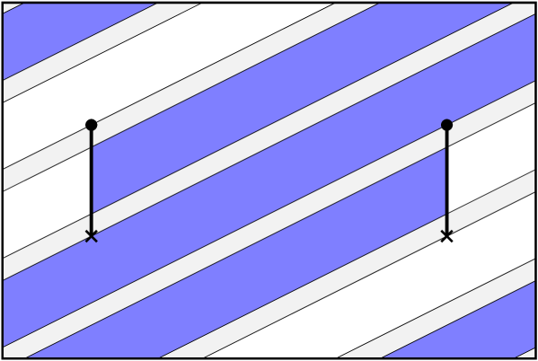
Figure 3: Three cylinders of periodic orbits bounded by four saddle-connexions in the case $M=4,N=1$.

The results of this section can be summed up as follows. We set

$$s_{1}=h_{1}+h_{3}$$

$$s_{2}=h_{2}+h_{3},$$ (8)

so that $s_{1}$ and $s_{2}$ are integers. Then in each direction ${\bf v}$ defined by $(M,N)$ with $M$ and $N$ coprime, there are three cylinders of periodic orbits of lengths $w_{i}l_{p}$ and heights $(2b/M)h_{i}$ with $i=1,2,3$. The cylinders can be described by the following five characteristic numbers:

• the integers $w_{1}$ and $w_{2}$ (giving the lengths of the two short cylinders and the length $(w_{1}+w_{2})l_{p}$ of the long cylinder)

• the real number $h_{3}$ (giving the height $(2b/M)h_{3}$ of the long cylinder)

• the integers $s_{1}$ and $s_{2}$ (giving the heights $(2b/M)(s_{1}-h_{3})$ and
  $(2b/M)(s_{2}-h_{3})$ of the short cylinders).

Note that by definition of the $s_{i}$ we need to have $0<h_{3}<\min(s_{1},s_{2})$. Also note that the condition that the sum of the areas of the cylinders be $4{\mathcal{A}}$ can be expressed as $s_{1}w_{1}+s_{2}w_{2}=q$.

3 Asymptotics for the periodic orbit lengths

Let us define ${\mathcal{F}}$ as the set of all 4-uples $(w_{1},w_{2},s_{1},s_{2})\in{(\mathbb{N}^{*})}^{4}$ such that $(s_{1},s_{2})$ are coprime and $s_{1}w_{1}+s_{2}w_{2}=q$. We say that a direction ${\bf v}$ belongs to the family $f\in{\mathcal{F}}$ if the three cylinders in the direction ${\bf v}$ have the characteristic numbers $w_{1},w_{2},s_{1},s_{2}$. The goal of this section is to calculate, for a fixed family $f\in{\mathcal{F}}$ and a fixed interval $I\subset[0,\min(s_{1},s_{2})[$, the asymptotics for the number ${\mathcal{N}}^{(q)}_{f,I}(l)$ of directions ${\bf v}$ belonging to the family $f$, such that $||{\bf v}||<l$ and such that the height $h_{3}$ of the third cylinder in the direction ${\bf v}$ belongs to the interval $I$.

3.1 Counting periodic orbits

The asymptotics for the number ${\mathcal{N}}^{(q)}(l)$ of cylinders of length less than $l$ have been calculated in [15]. These asymptotics are obtained by applying a Siegel-Veech formula to the space ${\mathcal{M}}_{q}(1,1)$ of $q$-fold coverings of the torus with two branch points and area 1. If $V(S)$ is the set of vectors associated with cylinders of periodic orbits on a ’stable’ $q$-fold torus cover $S$, then it is shown that there is a constant $\kappa(S)$ depending only on the connected component ${\mathcal{M}}(S)$ of ${\mathcal{M}}_{q}(1,1)$ containing $S$, such that

$$|V(S)\cap B(T)|\sim\pi\kappa T^{2},$$ (9)

where $|.|$ denotes the cardinal of a set and $B(T)$ is the ball of radius $T$ centered at the origin. The constant $\kappa$ is given by the following Siegel-Veech formula: for any continuous compactly supported $\varphi:{\mathbb{R}}^{2}\to\mathbb{R}$,

$$\frac{1}{\tilde{\mu}({\mathcal{M}}(S))}\int_{{\mathcal{M}}(S)}\hat{\varphi}\ d\tilde{\mu}=\kappa\int_{{\mathbb{R}}^{2}}\varphi,$$ (10)

where $\hat{\varphi}$ is the Siegel-Veech transform of $\varphi$ defined by

$$\hat{\varphi}(S)=\sum_{v\in V(S)}\varphi(v)$$ (11)

and $\tilde{\mu}$ is the measure on ${\mathcal{M}}_{q}(1,1)$ (Theorem 2.4 of [15]). This Theorem applies to the translation surface constructed from the barrier billiard, provided $S$ be a stable $q$-fold torus cover, which is true only if the height $\alpha$ of the barrier is irrational. It is shown that in this case ${\mathcal{M}}(S)$ is the set ${\mathcal{P}}_{q}(1,1)\subset{\mathcal{M}}_{q}(1,1)$ of primitive torus covers. The following asymptotics are then obtained (here we have a factor 1/16 differing from the factor in [15] because of our conventions for the counting of the time-reverse partner of a periodic orbit):

$${\mathcal{N}}^{(q)}(l)\sim c\frac{\pi l^{2}}{16{\mathcal{A}}}.$$ (12)

The constant $c$ is given by

$$c=\frac{q}{N_{q}}\sum_{r|q}\mu(r)\sum_{\genfrac{}{}{0.0pt}{}{(s_{1},s_{2})=1}{s_{1}u_{1}+s_{2}u_{2}=q/r}}u_{1}u_{2}(u_{1}+u_{2})\min(s_{1},s_{2})\left(\frac{1}{u_{1}^{2}}+\frac{1}{u_{2}^{2}}+\frac{1}{(u_{1}+u_{2})^{2}}\right)$$ (13)

(the gcd of $s,s^{\prime}$ will be noted either $\gcd(s,s^{\prime})$ or simply $(s,s^{\prime})$), and

$$N_{q}=\sum_{r|q}\mu(r)r^{2}\sum_{\genfrac{}{}{0.0pt}{}{(s_{1},s_{2})=1}{s_{1}u_{1}+s_{2}u_{2}=q/r}}u_{1}u_{2}(u_{1}+u_{2})\min(s_{1},s_{2})$$ (14)

(Proposition 4.14 of [15]). The constant $N_{q}$ is the number of primitive covers of degree $q$ of a surface of genus 2 with 2 branch points.

3.2 Siegel-Veech formula

The proof leading to Equation (12) can be adapted to any subset of $V(S)$ provided it varies linearly under $SL(2,\mathbb{R})$ action, i.e. provided the subset verifies $\forall g\in SL(2,\mathbb{R})$, $V(gS)=gV(S)$ (see Section 2 of [14] for more detail). To obtain the asymptotics for a fixed pair $F=(f,I)$ with $f=(w_{1},w_{2},s_{1},s_{2})\in{\mathcal{F}}$ and $I$ an interval, $I\subset[0,\min(s_{1},s_{2})[$, let us define $V_{F}(S)$ the set of vectors ${\bf v}\in{\mathbb{R}}^{2}$ defined by (4), such that the triple of cylinders in the direction ${\bf v}$ belongs to the family $f$, with $h_{3}\in I$. Then along the same lines of the proof of Theorem 2.4 in [15], one can show that when the height $\alpha$ of the barrier is irrational, the translation surface $S$ of the barrier billiard is a stable $q$-fold torus cover and

$$|V_{F}(S)\cap B(T)|\sim\pi\kappa_{F}T^{2},$$ (15)

where the constant $\kappa_{F}$ is given by the Siegel-Veech formula

$$\frac{1}{\tilde{\mu}({\mathcal{P}}_{q}(1,1))}\int_{{\mathcal{P}}_{q}(1,1)}\hat{\varphi_{F}}\ d\tilde{\mu}=\kappa_{F}\int_{{\mathbb{R}}^{2}}\varphi_{F},$$ (16)

with $\hat{\varphi_{F}}$ the Siegel-Veech transform

$$\hat{\varphi_{F}}(S)=\sum_{v\in V_{F}(S)}\varphi(v),$$ (17)

for some continuous compactly supported $\varphi:{\mathbb{R}}^{2}\to\mathbb{R}$.

3.3 Asymptotics for a family of periodic orbits

Following the steps leading from the Siegel-Veech formula (9)-(11) to the asymptotics (12)-(13) in [15], we can now derive asymptotics for the number of cylinders in each family $(f,I)$. Recall that ${\mathcal{N}}^{(q)}_{f,I}(l)$ is the number of directions ${\bf v}$ belonging to a family characterized by the numbers $f=(w_{1},w_{2},s_{1},s_{2})$, with a height $h_{3}\in I$, and such that $l_{p}$ given by Equation (5) is less than $l$. (Note that ${\mathcal{N}}^{(q)}_{f,I}(l)$ is a number of directions and not a number of cylinders.) Let $\rho_{f,I}(l)$ be the corresponding density. According to Equation (15), ${\mathcal{N}}^{(q)}_{f,I}(l)$ is proportional to $l^{2}$; we define the constant $c_{f,I}$ by

$${\mathcal{N}}^{(q)}_{f,I}(l)\sim c_{f,I}\frac{\pi l^{2}}{16{\mathcal{A}}}.$$ (18)

The proof leading to the asymptotics for ${\mathcal{N}}^{(q)}_{f,I}(l)$ is essentially the same as the proof in [15], section 4.4, provided we replace the counting functions of the cylinders in [15] by counting functions of directions in which the cylinders belong to the family $(f,I)$ we are interested in. We take $\varphi$ to be the characteristic function of a disc of radius $\epsilon$ in ${\mathbb{R}}^{2}$. Therefore its Siegel-Veech transform $\hat{\varphi}$, as defined by (17), counts the number of directions on $S$ in which the cylinders belong to family $(f,I)$ and such that $l_{p}<\epsilon$. For $\epsilon$ small enough, the Siegel-Veech formula (16) is equivalent to

$$\pi\epsilon^{2}c_{f,I}=\zeta(2)\frac{1}{\tilde{\mu}({\mathcal{P}}_{q}(1,1))}\int_{{\mathcal{P}}_{q}(1,1)}\tilde{\varphi_{F}}\ d\tilde{\mu},$$ (19)

where $\zeta$ is the Riemann Zeta function and

$$\tilde{\varphi}_{f,I}(S)=\left\{\begin{array}[]{cl}1&\textrm{ \ \ \ if the cylinders in the horizontal direction belong}\cr&\textrm{to the family $f$, if $h_{3}\in I$ and if}\ ||{\bf v}||<\epsilon\cr 0&\textrm{ \ \ \ otherwise.}\end{array}\right.$$ (20)

We define $\chi_{f,I}:{\mathbb{R}}^{2}\mapsto\mathbb{R}$ by

$$\chi_{f,I}(v)=\left\{\begin{array}[]{cl}1&\textrm{ \ \ \ if the cylinders in the horizontal direction belong}\cr&\textrm{to the family $f$, if $h_{3}\in I$ and if}\ ||{\bf v}||<\epsilon\sqrt{q}\cr 0&\textrm{ \ \ \ otherwise.}\end{array}\right.$$ (21)

Following [15], we parametrize ${\mathcal{P}}_{q}(1,1)$ and perform the integration in (19). Part of it can be related to the integral over $\chi_{f,I}$, which is $\int_{{\mathbb{R}}^{2}}\chi_{f,I}(v)\ dv=\pi\epsilon^{2}q$. The integration yields

$$\int_{{\mathcal{P}}_{q}(1,1)}\tilde{\varphi_{F}}\ d\tilde{\mu}=\frac{\pi\epsilon^{2}q}{q\zeta(2)}\sum_{r|(w_{1},w_{2})}\frac{\mu(r)}{r}w_{1}w_{2}(w_{1}+w_{2})|I|.$$ (22)

From [15] we get $\tilde{\mu}({\mathcal{P}}_{q}(1,1))=N_{q}/q$, with $N_{q}$ given by (14). Equation (19) finally gives

$$c_{f,I}=\frac{q}{N_{q}}\sum_{r|(w_{1},w_{2})}\frac{\mu(r)}{r}w_{1}w_{2}(w_{1}+w_{2})|I|,$$ (23)

where $|I|$ is the length of the interval $I$.

Equation (23) shows that $c_{f,I}$ depends on $I$ only through its length. Is is therefore convenient to introduce the density of directions $p=(M,N)$ corresponding to a family $f$ and such that $l_{p}<l$ and $h_{3}=h$:

$${\mathcal{N}}^{(q)}_{f,h}(l)\sim c_{f,h}\frac{\pi l^{2}}{16{\mathcal{A}}},$$ (24)

with $c_{f,h}$ given by

$$c_{f,h}=\frac{q}{N_{q}}\sum_{r|q}\frac{\mu(r)}{r}w_{1}w_{2}(w_{1}+w_{2})\theta_{f}(h)$$ (25)

for any family $f=(w_{1},w_{2},s_{1},s_{2})$ of ${\mathcal{F}}$ and $h\in\mathbb{R}$. The function $\theta_{f}$ is the characteristic function of the interval $[0,\min(s_{1},s_{2})[$. The density of primitive periodic orbit lengths for the family $f\in{\mathcal{F}}$ and $h\in\mathbb{R}$ is

$$\rho_{pp,f,h}(l)\sim c_{f,h}\frac{3l}{4\pi{\mathcal{A}}}.$$ (26)

It is easy to verify that the expression (24) of ${\mathcal{N}}^{(q)}_{f,h}(l)$ is consistent with the total number ${\mathcal{N}}^{(q)}(l)$ of pencils of periodic orbits with length less than $l$. This comes from the fact that any pencil of periodic orbits contributing to ${\mathcal{N}}^{(q)}(l)$ belongs to a certain family $f$ and has a length $w_{i}l_{p}\leq l$, which implies that $l_{p}\leq l/w_{i}$. Therefore

$${\mathcal{N}}^{(q)}(l) = \sum_{f\in{\mathcal{F}}}\int dh\sum_{i=1}^{3}{\mathcal{N}}^{(q)}_{f,h}(l/w_{i})$$ (27)

$$\sim \sum_{f\in{\mathcal{F}}}\int dh\ c_{f,h}\frac{\pi l^{2}}{16{\mathcal{A}}}\left(\frac{1}{w_{1}^{2}}+\frac{1}{w_{2}^{2}}+\frac{1}{(w_{1}+w_{2})^{2}}\right).$$

Using Equation (25), we obtain, after integration over $h$,

$${\mathcal{N}}^{(q)}(l) \sim \frac{\pi l^{2}}{16{\mathcal{A}}}\frac{q}{N_{q}}\sum_{\genfrac{}{}{0.0pt}{}{(s_{1},s_{2})=1}{s_{1}w_{1}+s_{2}w_{2}=q}}\sum_{r|(w_{1},w_{2})}\frac{\mu(r)}{r}w_{1}w_{2}(w_{1}+w_{2})$$ (28)

$$\times\min(s_{1},s_{2})\left(\frac{1}{w_{1}^{2}}+\frac{1}{w_{2}^{2}}+\frac{1}{(w_{1}+w_{2})^{2}}\right).$$

Making the substitution $w_{i}=ru_{i}$ and inverting the two sums, we get exactly the expression given by Equations (12) and (13).

4 Calculation of the form factor at $\tau=0$

4.1 Definitions

The spectrum $\{E_{n},n\in\mathbb{N}\}$ of a quantum billiard can be described by the density

$$d(E)\equiv\sum_{n}\delta(E-E_{n}).$$ (29)

The two-point correlation form factor is defined as the Fourier transform of the two-point correlation function of the density of states:

$$K_{2}(\tau)=\int_{-\infty}^{\infty}\frac{d\epsilon}{\bar{d}}\langle d(E+\epsilon/2)d(E-\epsilon/2)\rangle_{\textrm{c}}e^{2i\pi\bar{d}\tau\epsilon}.$$ (30)

Here the product of the densities is averaged over an energy window of width $\Delta E\gg 1/\bar{d}$ centered around $E=k^{2}$ and such that $\Delta E\ll E$. If ${\mathcal{A}}$ is the area of the billiard, $\bar{d}={\mathcal{A}}/4\pi$ is the non-oscillating part of the density of states. The subscript c means that one only considers the connected part of the correlation function. It can be argued that in the case of pseudo-integrable systems, the leading term of the semiclassical expansion of $K_{2}(\tau)$ at small argument ($\tau\to 0$) is given in the diagonal approximation by the contribution of periodic orbits only: $K_{2}(\tau)=K^{\textrm{diag}}(\tau)+O(\tau)$, with

$$K^{\textrm{diag}}(\tau)=\frac{1}{8\pi^{2}\bar{d}}\sum_{p}\frac{|S_{p}|^{2}}{l_{p}}\delta(l_{p}-4\pi k\bar{d}\tau)$$ (31)

(see [12] for the derivation of this expression, based on heuristic arguments). The sum is performed over all pencils of periodic orbits $p$ of length $l_{p}$. In general, there can be several pencils having exactly the same length: in Equation (31), $S_{p}$ is the sum of the areas occupied by all pencils having, when (possibly) multiply repeated, a length $l_{p}$. The aim of the present section is to calculate the semiclassical form factor at small arguments (31), using the result (26) for the distribution of pencils of periodic orbits in the barrier billiard. Let us take a $C^{\infty}$, compactly supported test function and integrate the distribution $K^{\textrm{diag}}(\tau)$ over $\tau$. If the density of periodic pencils depends linearly on $l$ (as is the case for the barrier billiard or the rectangular billiard), the integration over families of periodic orbits yields $K^{\textrm{diag}}(\tau)=\lambda\Theta(\tau)$, where $\lambda$ is a constant and $\Theta$ the Heaviside step function. In such a case, we define $\overline{K_{2}(0)}=\lambda$.

As an introduction, we first deal with the simpler case of a rectangular billiard.

4.2 Rectangular billiard

In the case of the rectangular billiard, discussed in section 2.1, the periodic orbits have lengths $nl_{pp}$, where $l_{pp}$ is given by (1) with $(M,N)$ coprime, and $n\in\mathbb{N}$ is the repetition number. The area of each pencil of primitive periodic orbits $pp$ is $A_{pp}=4{\mathcal{A}}$. When the sides $a$ and $b$ of the rectangle are incommensurable, there is only one pencil of length $l_{pp}$ and therefore in Equation (31) $S_{p}=4{\mathcal{A}}$. Equation (31) becomes

$$K^{\textrm{diag}}(\tau)=\frac{1}{8\pi^{2}\bar{d}}\sum_{pp}\sum_{n}\frac{|4{\mathcal{A}}|^{2}}{n^{2}l_{pp}}\delta(l_{pp}-4\pi k\bar{d}\tau/n)$$ (32)

hence (using the fact that $\bar{d}={\mathcal{A}}/4\pi$ and turning the sum over $pp=(M,N)$ with $M$ and $N$ coprime into an integral over $l$ with density $\rho_{pp}(l)$)

$$K^{\textrm{diag}}(\tau)=\frac{8{\mathcal{A}}}{\pi}\sum_{n}\int_{0}^{\infty}dl\ \frac{1}{n^{2}l}\rho_{pp}(l)\delta(l-4\pi k\bar{d}\tau/n)$$ (33)

The density $\rho_{pp}(l)$ of periodic orbits is given by Equation (3) and yields $K^{\textrm{diag}}(\tau)=1$, as expected for integrable systems.

4.3 Barrier billiard

In the case of the barrier billiard, the periodic orbits have a length of the form $nwl_{p}$ with $l_{p}$ given by (5): here the primitive length is $wl_{p}$ and $n$ is the repetition number. Two pencils of periodic orbits $p$ and $p^{\prime}$ have the same length provided there exist repetition numbers $n$ and $n^{\prime}$ such that $nwl_{p}=n^{\prime}w^{\prime}l_{p^{\prime}}$. When $a$ and $b$ are incommensurable, this implies $p=p^{\prime}$, i.e. two pencils can have same length only if they are in the same direction. For a given direction $(M,N)$ with $M$ and $N$ coprime (which will now be labeled by $p$), there are three cylinders of area ${\mathcal{A}}_{i}$ and length $w_{i}l_{p}$, $1\leq i\leq 3$, and therefore $w,w^{\prime}$ belong to the set $\{w_{1},w_{2},w_{1}+w_{2}\}$. Equation (31) becomes

$$K^{\textrm{diag}}(\tau)=\frac{1}{8\pi^{2}\bar{d}}\sum_{p}\sum_{n}\frac{|S_{p,n}|^{2}}{nl_{p}}\delta(nl_{p}-4\pi k\bar{d}\tau)$$ (34)

where $l_{p}$ is given by (5) and $S_{p,n}$ is the sum over the ${\mathcal{A}}_{i}$ corresponding to a $w_{i}$ which divides $n$:

$$S_{p,n}=\sum_{i=1}^{3}{\mathcal{A}}_{i}\delta_{w_{i}|n},$$ (35)

with $\delta_{r|t}=1$ if $r$ divides $t$, 0 otherwise. Each area ${\mathcal{A}}_{i}$ is equal to $(2b/M)h_{i}\times(w_{i}l_{p})\cos\varphi_{p}$ ($\varphi_{p}$ is the angle between the orbit and the horizontal). This can be rewritten as

$${\mathcal{A}}_{i}=\frac{4{\mathcal{A}}}{q}h_{i}w_{i}$$ (36)

(note that since $\sum_{i}h_{i}w_{i}=s_{1}w_{1}+s_{2}w_{2}=q$, one has $\sum_{i}{\mathcal{A}}_{i}=4{\mathcal{A}}$, i.e. the total area of the translation surface, as expected). Therefore $S_{p,n}$ only depends of the five numbers $f=(w_{1},w_{2},s_{1},s_{2})$ and $h_{3}$, and can be rewritten:

$$S_{f,h_{3},n}=\frac{4{\mathcal{A}}}{q}\left[(s_{1}-h_{3})w_{1}\delta_{w_{1}|n}+(s_{2}-h_{3})w_{2}\delta_{w_{2}|n}+h_{3}(w_{1}+w_{2})\delta_{(w_{1}+w_{2})|n}\right].$$ (37)

The sum (34) over all periodic orbits can be partitioned into sums running over primitive pencils of periodic orbits $p(f,h)$ belonging to a family $f$ with a height of the long cylinder in $[h,h+dh[$; (34) becomes

$$K^{\textrm{diag}}(\tau)=\sum_{f\in{\mathcal{F}}}\int dh\sum_{p(f,h)}\sum_{n}\frac{|S_{p,n}|^{2}}{8\pi^{2}n^{2}l_{p}\bar{d}}\delta(l_{p}-\frac{4\pi k\bar{d}\tau}{n}).$$ (38)

Each of the sums corresponding to a family $f$ can be replaced, as in (33), by an integral with density $\rho_{pp,f,h}(l)$, and $S_{p,n}$ by $S_{f,h,n}$:

$$K^{\textrm{diag}}(\tau)=\sum_{f\in{\mathcal{F}}}\int dh\sum_{n}\frac{|S_{f,h,n}|^{2}}{8\pi^{2}n^{2}\bar{d}}\int_{0}^{\infty}dl\ \frac{\rho_{pp,f,h}(l)}{l}\delta(l-\frac{4\pi k\bar{d}\tau}{n}).$$ (39)

Replacing the density $\rho_{pp,f,h}$ by its expression (26), the integration over $l$ becomes straightforward and yields $K^{\textrm{diag}}(\tau)=\overline{K_{2}(0)}\Theta(\tau)$, where

$$\overline{K_{2}(0)}=\frac{1}{q^{2}}\frac{6}{\pi^{2}}\sum_{n}\frac{1}{n^{2}}\sum_{f\in{\mathcal{F}}}\int dh\left[(s_{1}-h)w_{1}\delta_{w_{1}|n}\right.$$ (40)

$$+\left.(s_{2}-h)w_{2}\delta_{w_{2}|n}+h(w_{1}+w_{2})\delta_{(w_{1}+w_{2})|n}\right]^{2}c_{f,h}$$

(we have used the fact that $\bar{d}={\mathcal{A}}/4\pi$). Expanding the square, we can perform the summation over $n$, using the identity

$$\sum_{n=1}^{\infty}\frac{\delta_{w_{1}|n}\delta_{w_{2}|n}}{n^{2}}=\frac{\pi^{2}}{6}\frac{\gcd(w_{1},w_{2})^{2}}{w_{1}^{2}w_{2}^{2}}.$$ (41)

The form factor can therefore be written, after simplifications using the fact that $\gcd(w_{1},w_{1}+w_{2})=\gcd(w_{2},w_{1}+w_{2})=\gcd(w_{1},w_{2})$, as

$$\overline{K_{2}(0)} = \frac{1}{q^{2}}\sum_{f\in{\mathcal{F}}}\int dh\ c_{f,h}\left[3h^{2}-2\left(s_{1}+s_{2}+q\frac{\gcd(w_{1},w_{2})^{2}}{w_{1}w_{2}(w_{1}+w_{2})}\right)h\right.$$ (42)

$$+ \left.s_{1}^{2}+s_{2}^{2}+2s_{1}s_{2}\frac{\gcd(w_{1},w_{2})^{2}}{w_{1}w_{2}}\right].$$

Replacing the weight $c_{f,h}$ by its expression (25), we can easily perform the integration over $h$, which consists of terms of the form

$$\int_{0}^{\min(s_{1},s_{2})}dh\ h^{\nu}=\frac{\min(s_{1},s_{2})^{\nu+1}}{\nu+1}$$ (43)

for $\nu=0,1,2$. The form factor becomes

$$\overline{K_{2}(0)} = \frac{1}{qN_{q}}\sum_{\genfrac{}{}{0.0pt}{}{(s_{1},s_{2})=1}{s_{1}w_{1}+s_{2}w_{2}=q}}\sum_{r|(w_{1},w_{2})}\frac{\mu(r)}{r}w_{1}w_{2}(w_{1}+w_{2})\left[\min(s_{1},s_{2})^{3}\right.$$ (44)

$$- \left(s_{1}+s_{2}+q\frac{\gcd(w_{1},w_{2})^{2}}{w_{1}w_{2}(w_{1}+w_{2})}\right)\min(s_{1},s_{2})^{2}$$

$$+ \left.\left(s_{1}^{2}+s_{2}^{2}+2s_{1}s_{2}\frac{\gcd(w_{1},w_{2})^{2}}{w_{1}w_{2}}\right)\min(s_{1},s_{2})\right].$$

This sum can be evaluated with some cumbersome arithmetic manipulations; the calculation is given in the Appendix, and the final result is unexpectedly simple:

$$\overline{K_{2}(0)}=\frac{1}{2}+\frac{1}{q}.$$ (45)

There are several comments to make concerning this value. First, it is close to the result corresponding to semi-Poisson statistics $\overline{K_{2}(0)}=1/2$ [12]. This result is not valid for $q=2$, since in that case there is an additional symmetry in the billiard, with respect to the barrier, and the spectrum has to be desymmetrized. The calculation in this case has been done in [29] for a height of the barrier equal to $b/2$ (half the height of the rectangle), and yields $\overline{K_{2}(0)}=1/2$. The calculation for $q=2$ and a barrier with any height has been done in [18] using a different method, and also yields $\overline{K_{2}(0)}=1/2$.

The result (45) is similar to previously obtained results [12] for rational polygonal billiards having the Veech property. For instance for triangular billiards with angles $(\pi/2,\pi/n,\pi/2-\pi/n)$ the form factor at the origin was found to be between $1/3$ and $3/5$ [12]. Here the form factor lies between $1/2$ and $5/6$, which again is close to the semi-Poisson result.

Appendix

In this appendix, we want to evalute the quantity

$$\overline{K_{2}(0)}=\frac{1}{qN_{q}}\sum_{\genfrac{}{}{0.0pt}{}{(s_{1},s_{2})=1}{s_{1}w_{1}+s_{2}w_{2}=q}}\sum_{r|(w_{1},w_{2})}\frac{\mu(r)}{r}f(s_{1},s_{2},w_{1},w_{2},q),$$ (46)

where

$$f(s_{1},s_{2},w_{1},w_{2},q) = w_{1}w_{2}(w_{1}+w_{2})\left[\min(s_{1},s_{2})^{3}\right.$$ (47)

$$- \left.\left(s_{1}+s_{2}+q\frac{\gcd(w_{1},w_{2})^{2}}{w_{1}w_{2}(w_{1}+w_{2})}\right)\min(s_{1},s_{2})^{2}\right.$$

$$+ \left.\left(s_{1}^{2}+s_{2}^{2}+2s_{1}s_{2}\frac{\gcd(w_{1},w_{2})^{2}}{w_{1}w_{2}}\right)\min(s_{1},s_{2})\right].$$

The function $f$ is homogeneous, in the sense that it verifies

$$f(s_{1},s_{2},\lambda w_{1},\lambda w_{2},\lambda q)=f(\lambda s_{1},\lambda s_{2},w_{1},w_{2},\lambda q)=\lambda^{3}f(s_{1},s_{2},w_{1},w_{2},q).$$ (48)

In (46), the first sum goes over all integers $w_{i}\geq 1$ and $s_{i}\geq 1$, $i=1,2$, verifying $s_{1}w_{1}+s_{2}w_{2}=q$ and $\gcd(s_{1},s_{2})=1$. The number $N_{q}$ is given by (14). The first step is to exchange the sum over $(s_{i},w_{i})$ and the sum over $r$ in (46), and substitute $w_{i}=ru_{i}$: using the homogeneity of $f$, we get

$$\overline{K_{2}(0)}=\frac{1}{qN_{q}}\sum_{r|q}\mu(r)r^{2}\sum_{\genfrac{}{}{0.0pt}{}{(s_{1},s_{2})=1}{s_{1}u_{1}+s_{2}u_{2}=q/r}}f(s_{1},s_{2},u_{1},u_{2},\frac{q}{r}),$$ (49)

To get rid of the co-primality condition on $(s_{1},s_{2})$ we use the exclusion-inclusion principle, which for any function $\varphi$ gives

$$\sum_{(s,s^{\prime})=1}\varphi(s,s^{\prime})=\sum_{s,s^{\prime}=1}^{\infty}\sum_{t=1}^{\infty}\mu(t)\varphi(ts,ts^{\prime}).$$ (50)

This allows to rewrite the form factor as

$$\overline{K_{2}(0)} = \frac{1}{qN_{q}}\sum_{r|q}\mu(r)r^{2}\sum_{t=1}^{\infty}\mu(t)\sum_{ts_{1}u_{1}+ts_{2}u_{2}=q/r}f(ts_{1},ts_{2},u_{1},u_{2},\frac{q}{r})$$

$$= \frac{1}{qN_{q}}\sum_{r|q}\mu(r)r^{2}\sum_{t|q}\mu(t)t^{3}\sum_{s_{1}u_{1}+s_{2}u_{2}=q/(rt)}f(s_{1},s_{2},u_{1},u_{2},\frac{q}{rt})$$

Here the sum over $t$ from 1 to $\infty$ has been replaced by a sum over $t|q$ since for all the other values of $t$ there is no value of $(s_{1},s_{2},u_{1},u_{2})$ fulfilling the condition $ts_{1}u_{1}+ts_{2}u_{2}=q/r$. Again, the homogeneity of $f$ (Equation (47)) has been used. Setting $d=rt$ we get

$$\overline{K_{2}(0)}=\frac{1}{qN_{q}}\sum_{d|q}\left(\sum_{t|d}\mu(t)\mu(\frac{d}{t})d^{2}t\right)\sum_{s_{1}u_{1}+s_{2}u_{2}=q/d}f(s_{1},s_{2},u_{1},u_{2},\frac{q}{d}).$$

We need to evaluate

$$\overline{K_{2}(0)}=\frac{1}{qN_{q}}\sum_{d|q}\left(\sum_{t|d}\mu(t)\mu(\frac{d}{t})d^{2}t\right)(G_{q/d}+H_{q/d}),$$ (52)

where

$$G_{n} \equiv \sum_{s_{1}u_{1}+s_{2}u_{2}=n}u_{1}u_{2}(u_{1}+u_{2})\left[\min(s_{1},s_{2})^{3}\right.$$

$$- \left.\left(s_{1}+s_{2}\right)\min(s_{1},s_{2})^{2}+\left(s_{1}^{2}+s_{2}^{2}+2s_{1}s_{2}\right)\min(s_{1},s_{2})\right]$$

and

$$H_{n} \equiv \sum_{s_{1}u_{1}+s_{2}u_{2}=n}u_{1}u_{2}(u_{1}+u_{2})\left[-q\frac{\gcd(u_{1},u_{2})^{2}}{u_{1}u_{2}(u_{1}+u_{2})}\min(s_{1},s_{2})^{2}\right.$$ (54)

$$\hskip 85.35826pt+\left.2s_{1}s_{2}\frac{\gcd(u_{1},u_{2})^{2}}{u_{1}u_{2}}\min(s_{1},s_{2})\right].$$

The quantities $G_{n}$ and $H_{n}$ will be evaluated separately. This evaluation will require the use of a theorem proved in [23]:
Theorem. Let $f:\mathbb{Z}$${}^{4}\rightarrow\mathbb{C}$ such that

$$f(a,b,x,y)-f(x,y,a,b)=f(-a,-b,x,y)-f(x,y,-a,-b)$$ (55)

for all integers $a,b,x$ and $y$. Then for $n\in\mathbb{N}$, $n\geq 1$,

$$\sum_{\genfrac{}{}{0.0pt}{}{a,b,x,y\geq 1}{ax+by=n}}\left[f(a,b,x,-y)-f(a,-b,x,y)+f(a,a-b,x+y,y)\right.$$

$$-\left.f(a,a+b,y-x,y)+f(b-a,b,x,x+y)-f(a+b,b,x,x-y)\right]$$

$$=\sum_{d|n}\sum_{x=1}^{d-1}\left[f(0,\frac{n}{d},x,d)+f(\frac{n}{d},0,d,x)+f(\frac{n}{d},\frac{n}{d},d-x,-x)\right.$$

$$-\left.f(x,x-d,\frac{n}{d},\frac{n}{d})-f(x,d,0,\frac{n}{d})-f(d,x,\frac{n}{d},0)\right].$$ (56)

a. Evaluation of $G_{n}$

We can immediately point out that the identity

$$\min(s_{1},s_{2})^{2}-(s_{1}+s_{2})\min(s_{1},s_{2})=-s_{1}s_{2},$$ (57)

valid for any integers $s_{1}$ and $s_{2}$, allows to simplify $G_{n}$. We now need to evaluate the sum

$$G_{n}=\sum_{s_{1}u_{1}+s_{2}u_{2}=n}u_{1}u_{2}(u_{1}+u_{2})\min(s_{1},s_{2})\left(s_{1}^{2}+s_{2}^{2}-s_{1}s_{2}\right).$$ (58)

for any integer $n$. Writing $\min(a,b)=\frac{1}{2}(a+b-|a-b|)$, we have

$$G_{n} = \frac{1}{2}\sum_{s_{1}u_{1}+s_{2}u_{2}=n}u_{1}u_{2}\left[s_{1}^{3}u_{2}+s_{2}^{3}u_{1}-\frac{1}{3}(s_{1}^{3}u_{1}+s_{2}^{3}u_{2})\right.$$

$$- \left.\vphantom{\frac{1}{2}}(u_{1}+u_{2})(s_{1}^{2}+s_{2}^{2}-s_{1}s_{2})|u_{1}-u_{2}|\right]+\frac{2}{3}\sum_{s_{1}u_{1}+s_{2}u_{2}=n}u_{1}u_{2}(s_{1}^{3}u_{1}+s_{2}^{3}u_{2}).$$

The first sum in (a. Evaluation of $G_{n}$) can be evaluated by applying Theorem (Appendix) to the function

$$f(a,b,x,y)=\frac{1}{3}\left(xy-\frac{|xy|}{2}\right)\left|(a-b)(x-y)\right|(a^{2}+b^{2}-ab)$$ (60)

and is equal to

$$\frac{n^{2}(n-1)}{18}\sum_{d|n}d.$$ (61)

The second sum in (a. Evaluation of $G_{n}$) can be evaluated by applying Theorem (Appendix) to the function $f(a,b,x,y)=b^{2}y^{4}-b^{2}xy^{3}$ (see [23]). It gives

$$\frac{4}{3}\sum_{ax+by=n}a^{3}x^{2}y=\frac{n^{2}}{18}\sum_{d|n}\left(3d^{3}+(1-4n)d\right).$$ (62)

Finally we get

$$G_{n}=\frac{n^{2}}{6}\sum_{d|n}\left(d^{3}-nd\right).$$ (63)

If we now evaluate the quantity

$$\sum_{s_{1}u_{1}+s_{2}u_{2}=n}u_{1}u_{2}(u_{1}+u_{2})\min(s_{1},s_{2})=\frac{1}{2}\sum_{s_{1}u_{1}+s_{2}u_{2}=n}u_{1}u_{2}\left[s_{1}u_{2}+s_{2}u_{1}\vphantom{\frac{1}{2}}\right.$$

$$\left.-\frac{1}{3}(s_{1}u_{1}+s_{2}u_{2})-(u_{1}+u_{2})|u_{1}-u_{2}|\right]+\frac{2n}{3}\sum_{s_{1}u_{1}+s_{2}u_{2}=n}u_{1}u_{2},$$ (64)

the first sum is given by Theorem (Appendix) applied to the function

$$f(a,b,x,y)=\frac{1}{3}\left(xy-\frac{|xy|}{2}\right)\left|(a-b)(x-y)\right|$$ (65)

and the second one is given by Theorem (Appendix) applied to the function
$f(a,b,x,y)=nxy/3$; altogether, this gives

$$\sum_{s_{1}u_{1}+s_{2}u_{2}=n}u_{1}u_{2}(u_{1}+u_{2})\min(s_{1},s_{2})=\frac{n}{3}\sum_{d|n}\left(d^{3}-nd\right).$$ (66)

Together with Equation (63) we get

$$G_{n}=\frac{n}{2}\sum_{s_{1}u_{1}+s_{2}u_{2}=n}u_{1}u_{2}(u_{1}+u_{2})\min(s_{1},s_{2}).$$ (67)

b. Evaluation of $H_{n}$

We want to evaluate

$$H_{n} = \sum_{s_{1}u_{1}+s_{2}u_{2}=n}u_{1}u_{2}(u_{1}+u_{2})\min(s_{1},s_{2})\hskip 113.81102pt$$ (68)

$$\hskip 56.9055pt\left(-n\frac{\min(s_{1},s_{2})}{u_{1}u_{2}(u_{1}+u_{2})}+\frac{2s_{1}s_{2}}{u_{1}u_{2}}\right)\gcd(u_{1},u_{2})^{2}$$

for any integer $n$. Summing over all the possible values $r$ of the $\gcd$ of $u_{1}$ and $u_{2}$, and substituting $u_{i}=rv_{i}$, we have

$$H_{n}=\sum_{r|n}\sum_{\genfrac{}{}{0.0pt}{}{(v_{1},v_{2})=1}{s_{1}v_{1}+s_{2}v_{2}=n/r}}r^{3}v_{1}v_{2}(v_{1}+v_{2})\min(s_{1},s_{2})\left(-\frac{n}{r}\frac{\min(s_{1},s_{2})}{v_{1}v_{2}(v_{1}+v_{2})}+\frac{2s_{1}s_{2}}{v_{1}v_{2}}\right).$$ (69)

Then, as before, the co-primality condition can be expressed by a sum over $t$ (see Equation (50)). Restricting the sum over $t$ as before, we get

$$H_{n} = \sum_{r|n}\sum_{t|n}\mu(t)r^{3}t\sum_{s_{1}v_{1}+s_{2}v_{2}=n/(rt)}v_{1}v_{2}(v_{1}+v_{2})\min(s_{1},s_{2})\hskip 56.9055pt$$ (70)

$$\hskip 142.26378pt\left(-\frac{n}{rt}\frac{\min(s_{1},s_{2})}{v_{1}v_{2}(v_{1}+v_{2})}+\frac{2s_{1}s_{2}}{v_{1}v_{2}}\right).$$

Setting $d=rt$ we get

$$H_{n} = \sum_{d|n}\left(\sum_{t|d}\mu(t)\frac{d^{3}}{t^{2}}\right)\sum_{s_{1}v_{1}+s_{2}v_{2}=n/d}v_{1}v_{2}(v_{1}+v_{2})\min(s_{1},s_{2})\hskip 56.9055pt$$ (71)

$$\hskip 142.26378pt\left(-\frac{n}{d}\frac{\min(s_{1},s_{2})}{v_{1}v_{2}(v_{1}+v_{2})}+\frac{2s_{1}s_{2}}{v_{1}v_{2}}\right).$$

Let us now evaluate, for any integer $m$, the quantity

$$K_{m} = \sum_{s_{1}v_{1}+s_{2}v_{2}=m}v_{1}v_{2}(v_{1}+v_{2})\min(s_{1},s_{2})\left(-m\frac{\min(s_{1},s_{2})}{v_{1}v_{2}(v_{1}+v_{2})}+\frac{2s_{1}s_{2}}{v_{1}v_{2}}\right)$$ (72)

$$= -m\sum_{s_{1}v_{1}+s_{2}v_{2}=m}\min(s_{1},s_{2})^{2}+2\sum_{s_{1}v_{1}+s_{2}v_{2}=m}s_{1}s_{2}(v_{1}+v_{2})\min(s_{1},s_{2}).$$

Let

$$L_{m} = \sum_{s_{1}v_{1}+s_{2}v_{2}=m}(2s_{1}s_{2}-v_{1}v_{2})(v_{1}+v_{2})\min(s_{1},s_{2})$$

$$= \sum_{s_{1}v_{1}+s_{2}v_{2}=m}(2v_{1}v_{2}(s_{1}+s_{2})\min(v_{1},v_{2})-v_{1}v_{2}(v_{1}+v_{2})\min(s_{1},s_{2}))$$

after exchanging $(s_{1},s_{2})$ and $(v_{1},v_{2})$ in the first half of the right member. Writing $\min(a,b)=\frac{1}{2}(a+b-|a-b|)$ and applying Theorem (Appendix) to the function

$$f(a,b,x,y)=-\frac{1}{2}\left|ab(a-b)(x-y)\right|$$ (74)

one gets

$$L_{m}=m\sum_{d|m}\sum_{x=1}^{d-1}x(d-x).$$ (75)

Applying Theorem (Appendix) to the function

$$f(a,b,x,y)=\frac{ab-\left|ab\right|}{2}$$ (76)

one gets

$$\sum_{s_{1}v_{1}+s_{2}v_{2}=m}\min(s_{1},s_{2})^{2}=\sum_{d|m}\sum_{x=1}^{d-1}x(d-x).$$ (77)

This proves that

$$K_{m}=\sum_{s_{1}v_{1}+s_{2}v_{2}=m}v_{1}v_{2}(v_{1}+v_{2})\min(s_{1},s_{2})$$ (78)

and therefore

$$H_{n}=\sum_{d|n}\left(\sum_{t|d}\mu(t)\frac{d^{3}}{t^{2}}\right)\sum_{s_{1}v_{1}+s_{2}v_{2}=n/d}v_{1}v_{2}(v_{1}+v_{2})\min(s_{1},s_{2}).$$ (79)

c. Calculation of $\overline{K_{2}(0)}$

The evaluation of (52) will require to introduce the functions

$$f(n)=\frac{\mu(n)}{n}\ \ \ \ \ \ \ \textrm{and}\ \ \ \ g(n)=\sum_{d|n}\frac{\mu(d)}{d^{2}}$$ (80)

For $f_{1}$ and $f_{2}$ two arithmetic functions, the Dirichlet convolution is defined by

$$f_{1}*f_{2}(n)=\sum_{d|n}f_{1}(d)f_{2}(\frac{n}{d}).$$ (81)

Replacing the expressions found for $G_{q/d}$ and $H_{q/d}$ in Equation (52) we get

$$\overline{K_{2}(0)} = \frac{1}{qN_{q}}\sum_{d|q}(f*\mu)(d)d^{3}\left\{\sum_{s_{1}u_{1}+s_{2}u_{2}=q/d}\left(\frac{q}{2d}\right)u_{1}u_{2}(u_{1}+u_{2})\min(s_{1},s_{2})\right.$$ (82)

$$+ \left.\sum_{d^{\prime}|q/d}d^{\prime 3}g(d^{\prime})\sum_{s_{1}u_{1}+s_{2}u_{2}=q/dd^{\prime}}u_{1}u_{2}(u_{1}+u_{2})\min(s_{1},s_{2})\right\}.$$

Rewriting the constant $N_{q}$ given by (14), using the inclusion-exclusion principle and following the steps from Equations (49) to (Appendix), we get

$$N_{q}=\sum_{d|q}(f*\mu)(d)d^{2}\sum_{s_{1}u_{1}+s_{2}u_{2}=q/d}u_{1}u_{2}(u_{1}+u_{2})\min(s_{1},s_{2}).$$ (83)

We see that the first term in (82) is equal to 1/2. If we set $\delta=dd^{\prime}$, the second term gives

$$\frac{1}{qN_{q}}\sum_{\delta|q}(\frac{\delta}{d})^{3}\left(\sum_{d|\delta}(f*\mu)(d)g(\frac{\delta}{d})\right)\sum_{s_{1}u_{1}+s_{2}u_{2}=q/\delta}u_{1}u_{2}(u_{1}+u_{2})\min(s_{1},s_{2}).$$ (84)

But

$$\sum_{d|\delta}(f*\mu)(d)g(\frac{\delta}{d})=[(f*\mu)*g](\delta)=[f*(\mu*g)](\delta)$$ (85)

by associativity of Dirichlet convolution, and

$$(\mu*g)(\delta)=\frac{\mu(\delta)}{\delta^{2}}$$ (86)

by Moebius inversion formula. Finally the term (84) simplifies to $1/q$, which completes the proof.

References

• [1] Agam, O., Altshuler, B.L., Andreev, A.V.: Spectral Statistics from disordered to chaotic systems. Phys. Rev. Lett 75, 4389 (1995).
• [2] Andreev, A. V., Altshuler, B.L.: Spectral Statistics beyond Random Matrix Theory. Phys. Rev. Lett. 75, 902-905 (1995).
• [3] Balian, R., Bloch, C.: Distribution of eigenfrequencies for the wave equation in a finite domain: Eigenfrequency density oscillations. Ann. Phys. (N.Y.) 69, 76 (1972).
• [4] Berry, M. V.: Semiclassical theory of spectral rigidity. Proc. Roy. Soc. A 400, 229 (1985).
• [5] Richens, P. J., Berry, M. V.: Pseudointegrable systems in classical and quantum mechanics. Physica D 2, 495 (1981).
• [6] Berry, M. V., Tabor, M.: Closed Orbits and the Regular Bound Spectrum. Proc. Roy. Soc. Lond. A 349, 101-123 (1976).
• [7] Berry, M. V., Tabor, M.: Level clustering in the regular spectrum. Proc. Roy. Soc. Lond. A 356, 375-94 (1977).
• [8] Bohigas, O., Giannoni, M.-J., Schmit, C.: Characterization of Chaotic Quantum Spectra and Universality of Level Fluctuation Laws. Phys. Rev. Lett. 52, 1 (1984).
• [9] Bogomolny, E. B.: Action correlations in integrable systems. Nonlinearity 13, 947-972 (2000).
• [10] Bogomolny, E., Gerland, U., Schmit, C.: Models of intermediate spectral statistics. Phys. Rev. E 59, R1315 (1999).
• [11] Bogomolny, E., Pavloff, N., Schmit, C.: Diffractive corrections in the trace formula for polygonal billiards. Phys. Rev. E 61, 3689 (2000).
• [12] Bogomolny, E., Giraud, O., Schmit, C.: Periodic orbits contribution to the 2-point correlation form factor for pseudo-integrable systems. Comm. Math. Phys. 222, 327 (2001).
• [13] Casati, G., Prosen, T.: Mixing Property of Triangular Billiards. Phys. Rev. Lett. 83, 4729-4732 (1999).
• [14] Eskin, A., Masur, H.: Asymptotic formulas on flat surfaces. Ergod. Theor. & Dyn. Sys. 21, 443-478 (2001).
• [15] Eskin, A., Masur, H., Schmoll, M.: Billiards in Rectangles with Barriers. Duke Math. J. 118, 427-463 (2003).
• [16] Eskin, A., Masur, H., Zorich, A.: Moduli spaces of abelian differentials: the principal boundary, counting problems and the Siegel-Veech constants. Publications IHES 97, 61-179 (2003).
• [17] Giraud, O., Marklof, J., O’Keefe, S.: Intermediate statistics in quantum maps. J. Phys. A: Math. Gen. 37 no 28, L303-L311 (2004).
• [18] Giraud, O.: Statistiques spectrales des systΓ¨mes difractifs. PhD Thesis, UniversitΓ© Paris XI (2002).
• [19] Gutkin, E., Judge, C.: Affine Mappings of Translation Surfaces: Geometry and Arithmetic. Duke Math. J. 103, 191-213 (2000).
• [20] Gutzwiller, M. C.: The semi-classical quantization of chaotic hamiltonian systems. In Chaos and Quantum Mechanics, Giannoni, M.-J., Voros, A. and Zinn-Justin, J. eds., Les Houches Summer School Lectures LII, 1989 (North Holland, Amsterdam, 1991), p. 87.
• [21] Hannay, J. H., McCraw, . J.: Barrier billiards - a simple pseudo-integrable system. J. Phys. A: Math. Gen. 23, 887-900 (1990).
• [22] Hannay, J. H., Ozorio de Almeida, A. M.: Periodic orbits and a correlation function for the semiclassical density of states. J. Phys. A: Math. Gen. 17, 3429-3440 (1984).
• [23] Huard, J.G., Ou, Z.M., Spearman, B. K., Williams, K.S.: Elementary Evaluation of Certain Convolution Sums involving Divisor Functions. Number Theory for the Millennium II, A K Peters publisher, Natick, Massachusetts, 229-274 (2002).
• [24] Marklof, J.: Spectral Form Factors of Rectangle Billiards. Comm. Math. Phys. 199, 169 (1998).
• [25] Masur, H.: The Growth Rate of Trajectories of a Quadratic Differential. Ergod. Theor. & Dyn. Sys. 10, 151-176 (1990).
• [26] Sieber, M.: Geometrical theory of diffraction and spectral statistics. J. Phys. A: Math. Gen. 32, 7679-7689 (1999).
• [27] Veech, W. A.: TeichmΓΌller curves in moduli space, Eisenstein series and an application to triangular billiards. Invent. Math. 97 (1989), 553-583.
• [28] Vorobets, Y. B.: Planar structures and billiards in rational polygons: the Veech alternative. Russian Math. Surveys 51, 5 (1996), 779-817.
• [29] Wiersig, J.: Spectral Properties of Quantized Barrier Billiards. Phys. Rev. E 65 4627 (2002).
• [30] Zemlyakov, A. B., Katok, A. N.: Topological Transitivity of Billiards in Polygons. Math. Notes 18, 760-764 (1976).