STABILITY OF THOMSON’S
CONFIGURATIONS OF VORTICES ON A SPHERE

A. V. BORISOV
Faculty of Mechanics and Mathematics,
Department of Theoretical Mechanics Moscow State University
Vorob’ievy gory, 119899 Moscow, Russia
E-mail: borisov@uni.udm.ru
A. A. KILIN
Laboratory of Dynamical Chaos and Non Linearity,
Udmurt State University
Universitetskaya, 1, Izhevsk, Russia, 426034
E-mail: aka@uni.udm.ru

Abstract

In this work stability of polygonal configurations on a plane and sphere is investigated. The conditions of linear stability are obtained. A nonlinear analysis of the problem is made with the help of Birkhoff normalization. Some problems are also formulated.

1 A linear stability of Thomson’s configurations of vortices on a sphere

Motion equations of a system of $N$ point vortices on a sphere can be presented in the Hamiltonian form [1] with the Poisson bracket

$$\{\varphi_{i},\,\cos\theta_{k}\}=\frac{\delta_{ik}}{R^{2}\Gamma_{i}}$$ (1)

and the Hamiltonian

$$\begin{split}H=-\frac{1}{8\pi}\mathop{{\sum}^{\prime}}\limits_{i,\,k=1}^{N}\Gamma_{i}\Gamma_{k}\ln\left(4R^{2}\sin^{2}\frac{\gamma_{ik}}{2}\right)\mbox{, }\\ \cos\gamma_{ik}=\cos\theta_{i}\cos\theta_{k}+\sin\theta_{i}\sin\theta_{k}\cos(\varphi_{k}-\varphi_{i})\,,\end{split}$$ (2)

where $\theta_{i}$, $\varphi_{i}$ and $\Gamma_{i}$ are spherical coordinates and the intensity of the $i$-th vortex, $\gamma_{ik}$ is an angle between the $i$-th and the $k$-th vortices, $R$ is a radius of the sphere the prime denotes that $i\neq k$. Here and further all indices values from 1 to $N$. Motion equations of such a system have the form

$$\left\{\begin{aligned} \dot{\theta}_{k}&=-\frac{1}{4\pi R^{2}}\mathop{{\sum}^{\prime}}\limits_{i=1}^{N}\Gamma_{i}\frac{\sin\theta_{i}\sin(\varphi_{k}-\varphi_{i})}{1-\cos\gamma_{ik}}\,,\\ \sin\theta_{k}\dot{\varphi}_{k}&=\frac{1}{4\pi R^{2}}\mathop{{\sum}^{\prime}}\limits_{i=1}^{N}\Gamma_{i}\frac{\sin\theta_{k}\cos\theta_{i}-\cos\theta_{k}\sin\theta_{i}\cos(\varphi_{k}-\varphi_{i})}{1-\cos\gamma_{ik}}\,.\end{aligned}\right.$$ (3)

In the case of equal intensities $\Gamma_{i}$ the system is invariant with respect to the discrete group of permutations of vortices, and therefore allows different symmetric partial solutions. Let us consider partial solutions, which are analogous to the well known Thomson’s configurations on a plane. Then the vortices are located on the same latitude $\theta_{0}$ in the vertices of a regular $N$-gon and rotate around its center with the angular velocity $\omega$:

$$\theta_{i}=\theta_{0}=const\,,\qquad\varphi_{i}=\omega(\theta_{0})t+\frac{2\pi}{N}(i-1)\,,\qquad\omega(\theta_{0})=\frac{\Gamma(N-1)}{4\pi R^{2}}\frac{\cot\theta_{0}}{\sin\theta_{0}}\,.$$ (4)

Let us consider stability of these partial solutions in linear approximation. The study of stability of Thomson’s configurations of vortices on a plane in linear approximation was carried out by J. Thomson [2]. He has shown that they are stable in linear approximation for $N\leq 7$, and unstable for $N>7$. Let us take variations $\delta\theta_{i}$ and $\delta\varphi_{i}$ as

$$\theta_{i}=\theta_{0}+\delta\theta_{i}\,,\qquad\varphi_{i}=\omega(\theta_{0})t+\frac{2\pi}{N}(i-1)+\delta\varphi_{i}\,.$$ (5)

The linearized equations for $\delta\theta_{i}$ and $\delta\varphi_{i}$ are autonomous and have the form:

$$\left\{\begin{aligned} \delta\dot{\theta}_{k}&=\frac{\Gamma}{4\pi R^{2}}\frac{1}{2\sin\theta_{0}}A_{ki}\delta\varphi_{i}\,,\\ \sin\theta_{0}\delta\dot{\varphi}_{k}&=\frac{\Gamma}{4\pi R^{2}}\frac{1}{2\sin^{2}\theta_{0}}A_{ki}\delta\vartheta_{i}-\frac{\Gamma(N-1)}{4\pi R^{2}}\frac{1+\cos^{2}\theta_{0}}{\sin^{2}\theta_{0}}\delta\theta_{k}\,,\end{aligned}\right.$$ (6)

where $A$ is an $(N\times N)$-matrix with the elements

$$A_{ki}=\delta_{ki}\sum\limits_{m=1}^{N-1}\frac{1}{\sin^{2}\frac{\pi}{N}m}-(1-\delta_{ki})\frac{1}{\sin^{2}\frac{\pi}{N}(k-i)}\,.$$ (7)

By differentiating with respect to time, the equations (6) can be reduced to a system of $N$ second-order equations in the following form:

$$\delta\ddot{\varphi}_{k}=\Biggl{(}\frac{\Gamma}{8\pi R^{2}\sin^{2}\theta_{0}}\Biggr{)}^{2}\left(A_{kj}-2(N-1)(1+\cos^{2}\theta_{0})\delta_{kj}\right)A_{ji}\delta\varphi_{i}$$ (8)

(similar equations are obtained for $\theta_{k}$ under elimination of $\varphi_{k}$).

A solution of the equation (8) has the form

$$\delta\varphi_{k}=\sum\limits_{m}C^{(m)}_{k}e^{\Omega_{m}t},$$

where the constants $C_{k}^{(m)},\,\Omega_{m}$ are expressed through the eigenvalues and eigenvectors of the matrix $A_{ki}$. As in the case of a plane [3], the elements of $A_{ki}$ depend only on differences $(k-i)$, thus the matrix $A$ can be diagonalized by the Fourier transformation, and the eigenvalues of the matrix can be presented as

$$\lambda_{m}=2m(N-m)\,,\quad m=0,\,1,\,\ldots,\,\Bigl{[}\frac{N}{2}\Bigr{]}\,.$$ (9)

Each eigenvalue corresponds to two eigenvectors $\phi_{i}^{(m)}=\cos\left(\frac{2\pi m}{N}i\right)$ and $\psi_{i}^{(m)}=\sin\left(\frac{2\pi m}{N}i\right)$, ${i=1,\,\ldots,\,N}$. To the values $m=0$ and $m=\smash{\frac{N}{2}}$ (in case of even $N$), there corresponds a unique eigenvector $\phi_{i}^{(m)}$ [3].

Using (8), (9), we find frequencies $\Omega_{m}$

$$\Omega_{m} =\frac{\pm\Gamma\lambda_{m}^{\frac{1}{2}}}{8\pi R^{2}\sin^{2}\theta_{0}}\sqrt{\lambda_{m}-2(N-1)(1+\cos^{2}\theta_{0})}=$$ (10)

$$=\frac{\pm\Gamma\sqrt{m(N-m)}}{4\pi R^{2}\sin^{2}\theta_{0}}\sqrt{m(N-m)-(N-1)(1+\cos^{2}\theta_{0})}\,.$$

The presence of the zero frequency (10) at $m=0$ corresponds to instability of Thomson’s configurations in the absolute coordinate system. Indeed, under perturbations $\delta\theta_{i}$, $\delta\phi_{i}$ corresponding to $m=0$ the Thomson’s configuration (4) transforms into Thomson’s configuration, which is close to the latter and moves away from it linearly with time. Stability of relative motions of the vortices, from which we exclude the rotations of the system as solid-state configuration, are determined by the remained frequencies. It is necessary for the relative stability the remained frequencies $\Omega_{m}$ purely imaginary. It is obvious from (10) that the configurations (4) gradually lose their stability approaching the equator (i. e. with magnification of $\theta_{0}$).

Table 1 shows the boundaries of varying of the radicand in (10) for various $N$ with the maximum value $m(N-m)$ and also values of $\theta_{0}^{*}$, at which the radicand changes the sign.

For $N\geq 7$ there is always at least one frequency with a positive real part, hence, such configurations are unstable already in the linear approximation.

Table 1.

$N$ $\max(m(N-m))$ $m(N-m)-(N-1)(1+\cos^{2}\theta_{0})$ $\theta^{*}_{0}$ $\footnotesize\theta_{0}=0$ $\footnotesize\theta_{0}=\frac{\pi}{2}$ 2 1 $-1$ 0 $\frac{\pi}{2}$ 3 2 $-2$ 0 $\frac{\pi}{2}$ 4 4 $-2$ 1 $\arccos\frac{1}{\sqrt{3}}$ 5 6 $-2$ 2 $\frac{\pi}{4}$ 6 9 $-1$ 4 $\arccos\frac{2}{\sqrt{5}}$ 7 12 0 6 0 8 16 2 9 —

For $N=6,\,5,\,4,\,3$ and 2 and for $\theta_{0}\in(0,\,\theta_{0}^{*})$ all frequencies $\Omega_{m}$ are purely imaginary. Thus, under the above-mentioned conditions the specified configurations are stable in linear approximation. For $\theta_{0}\in[\theta_{0}^{*},\,\frac{\pi}{2}]$ these configurations are either unstable in linear approximation or consideration of higher order approximations (at $\theta_{0}=\theta_{0}^{*}$) is required for determination of stability.

2 A nonlinear stability of Thomson’s configurations on a sphere and a plane for $\boldsymbol{N=2,\,\ldots,\,6}$

The work by L. G. Khazin [4] introduced a proof of the Lyapunov stability of Thomson’s configurations in nonlinear statement on a plane. However, though the general theorem from the stability theory, proved by L. G. Khazin in this work is correct, its application to Thomson’s configurations on a plane is not appropriate. Zero frequencies considered by Khazin correspond to the motion of vortices as a whole and are not connected with the relative stability of Thomson’s configurations. Thus, the problem of stability of Thomson’s configurations on a plane in strict nonlinear statement was not solved.

Let us show the Lyapunov stability of Thomson’s configurations on a sphere and plane relatively to the perturbations of mutual distances between vortices (further we shall speak about “relative” stability) for $N=2,\,\ldots,\,6$.

The case of $\boldsymbol{N=2}$

The most general kind of motion of two vortices on a sphere (plane) is the uniform rotation around a motionless axis, which passes through the center of vorticity and the center of sphere (perpendicular plane) with preservation of the mutual distance [5, 6]. Under a small perturbation in this system the distance between vortices changes a little, but it is also preserved during the motion. Thus, Thomson’s configurations of two vortices are “relatively” Lyapunov stable both on a sphere and on a plane.

The case of $\boldsymbol{N=3}$

Let us consider a geometric interpretation of motion of three vortices on a sphere, that was used in [5, 6]. In Fig. 1 we represent the surface of integral

$$\boldsymbol{D}=a_{1}M_{1}+a_{2}M_{2}+a_{3}M_{3}$$

in the space of $M_{1},\,M_{2},\,M_{3}$, where $a_{i}=\frac{1}{\Gamma_{i}}$ are inverse intensities of vortices, and $M_{i}$ are squared distances between vortices. The triangular area presented in Fig. 1 is selected by the conditions $M_{i}\geq 0$.

We have painted the areas of nonphysical states, for which the triangle inequality is not fulfilled over, in black. The curves represent levels of the energy integral. Thomson’s configuration on this figure corresponds to the point $A$, where $M_{1}=M_{2}=M_{3}$. As we can see from the figure, under small perturbation of Thomson’s configuration the system starts moving along the level of the energy integral and $D$, close to the point $A$, which is bounded. Thus, after perturbation the system moves in a small neighbourhood of the point $A$, without leaving it. Analogous arguments can be carried out for the case of a plane. Hence, Thomson’s configurations of three vortices are “relatively” Lyapunov stable both on a sphere and on a plane.

The case of $\boldsymbol{N=4,\,5,\,6;\,\boldsymbol{\theta}_{0}\in[0,\,\boldsymbol{\theta}_{0}^{*})}$

To show the “relative” Lyapunov stability of Thomson’s configurations for $N=4,\,5,\,6$ and for ${\theta_{0}\in[0,\,\theta_{0}^{*})}$ let us diagonalize the quadratic part of the Hamiltonian $H_{2}$. Such a diagonalization, as it has been already said above, is carried out with the help of Fourier transformation given by the matrix

$$T_{kl}=\frac{1}{\sqrt{N}}e^{-\frac{2\pi i}{N}kl}\,.$$

After this diagonalization and elimination of a degree of freedom, corresponding to the motion of vortices as a solid-state configuration, we obtain:

$$H_{2}^{(4)}={} \frac{3\Gamma^{2}}{4\pi}\cot\theta_{0}(p_{1}^{2}+q_{1}^{2}+p_{2}^{2}+q_{2}^{2})+\frac{\Gamma^{2}}{2\pi}\frac{\sqrt{3\cos^{2}\theta_{0}-1}}{\sin\theta_{0}}(p_{3}^{2}+q_{3}^{2})\,,$$ (11)

$$H_{2}^{(5)}={} \frac{\Gamma^{2}}{\pi}\cot\theta_{0}(p_{1}^{2}+q_{1}^{2}+p_{2}^{2}+q_{2}^{2})+\frac{\Gamma^{2}}{2\pi}\frac{\sqrt{3(2\cos^{2}\theta_{0}-1)}}{\sin\theta_{0}}(p_{3}^{2}+q_{3}^{2}+p_{4}^{2}+q_{4}^{2})\,,$$

$$H_{2}^{(6)}={} \frac{5\Gamma^{2}}{4\pi}\cot\theta_{0}(p_{1}^{2}+q_{1}^{2}+p_{2}^{2}+q_{2}^{2})+\frac{3\Gamma^{2}}{4\pi}\frac{\sqrt{5\cos^{2}\theta_{0}-4}}{\sin\theta_{0}}(p_{5}^{2}+q_{5}^{2})+$$

$$+\frac{\Gamma^{2}}{2\pi}\frac{\sqrt{2(5\cos^{2}\theta_{0}-3)}}{\sin\theta_{0}}(p_{3}^{2}+q_{3}^{2}+p_{4}^{2}+q_{4}^{2})\,.$$

For $\theta_{0}\in(0,\,\theta_{0}^{*})$ the quadratic Hamiltonians (11) are positively defined and, consequently, can be used as Lyapunov functions. Thus, Thomson’s configurations of four, five and six vortices are “relatively” Lyapunov stable on a sphere in areas of their linear stability. Proceeding to limit $\theta_{0}\to 0$, it is also possible to show a “relative” Lyapunov stability on a plane.

3 The case $\boldsymbol{N=7}$ on a plane

Thomson’s configuration are unstable in linear approximation on a sphere in case $N=7$. On a plane the linear instability vanishes, but appears in the system of two zero frequencies with two-dimensional Jordan cells (the neutral case of a indifferent equilibrium). After diagonalization the quadratic Hamiltonian of the system takes the form

$$H_{2}=\frac{a}{2}(q_{1}^{2}+q_{2}^{2})+\frac{\omega_{1}}{2}(p_{3}^{2}+q_{3}^{2}+p_{4}^{2}+q_{4}^{2})+\frac{\omega_{2}}{2}(p_{5}^{2}+q_{5}^{2}+p_{6}^{2}+q_{6}^{2})\,,$$ (12)

where $a=\frac{3}{\pi},\,\omega_{1}=\frac{\sqrt{5}}{4\pi},\,\omega_{2}=\frac{3}{4\pi}$, and the values of $\Gamma$ and $R$ are assumed to be 1. It can be seen that this system has two resonances of type 1:1 (variables 3, 4 and 5, 6) and two zero frequencies with two-dimensional Jordan cells (variables 1 and 2). The Hamiltonian (12) is not positively defined, and, therefore, to study its stability it is necessary to investigate expansions of the Hamiltonian of higher order. For simplification of the Hamiltonian form we shall carry out the procedure of Deprit-Hori normalization (a detailed exposition of the procedure of Deprit-Hori normalization with the presence of zero frequencies with two-dimensional Jordan cells is presented in Appendix). After normalization the Hamiltonian of the third degree will have the form:

$$H_{3}=b(\frac{1}{2}(p_{1}-p_{2})(p_{4}^{2}+q_{4}^{2}-p_{3}^{2}-q_{3}^{2})+(p_{1}+p_{2})(p_{3}p_{4}+q_{3}q_{4}))\,,$$ (13)

where $b=0.0672552$. $H_{3}$ does not depend on the variables $p_{5},\,q_{5},\,p_{6},\,q_{6}$. Therefore, degrees of freedom, corresponding to these variables in approximation of the third order, are separated. Further we can consider a system with four degrees of freedom only.

To prove the instability of this system let us use a method of constructions of quasihomogeneous truncations of expansion of a Hamiltonian [7]. Thus for a system obtained from the initial one by quasihomogeneous truncation, we try to find sets of partial solutions as twisted rays $\sim\frac{1}{t^{\beta}}\sin(\omega\ln t+\alpha)$. We have considered basic quasihomogeneous truncations of a system of the third degree. However, non of them has a partial solution in form of twisted rays.

The book [7] presents constructions of increasing solutions for systems with two degrees of freedoms with resonances 1:1 and two zero frequencies with two-dimensional Jordan cells. In the case of resonance 1:1, to construct the increasing solutions we must have the terms of no less than the $4^{th}$ degree in variables, corresponding to the resonance; and in case of two zero frequencies with two-dimensional Jordan cells the terms must be no less than of the third degree. Due to particularity of the system and a large number of degrees of freedom, there is no such terms in this case, $H_{3}$ includes only “mixed” terms (depending both on variables, corresponding to the resonance 1:1, and on variables, corresponding to zero frequencies). Probably, this is the reason why it is impossible to find increasing partial solutions.

Motion equations of the system of the third degree have an invariant manifold

$$p_{2}=q_{2}=p_{3}=q_{3}=p_{4}=q_{4}=p_{5}=q_{5}=p_{6}=q_{6}=0\,.$$ (14)

The equations of motion on this manifold take the form:

$$\left\{\begin{aligned} \dot{p}_{1}&=-aq_{1}\,,\\ \dot{q}_{1}&=0\,.\end{aligned}\right.$$

A solution of the given system is a set of particular solutions, which increase linearly with time. However, a linearly increasing solution of the truncated system can not be extended to an asymptotically increasing solution of the complete system (which is possible for solutions in the form of twisted rays). Therefore, we shall consider the further expansion of the Hamiltonian up to terms of the fourth degree.

The normal form of the 4-th degree can be written as

$$H_{4}={} 0.943361q_{1}p_{1}q_{2}p_{2}+0.728898W_{12}R_{56}-0.518170W_{34}R_{56}+$$ (15)

$$+0.010176R_{56}^{2}-0.518170W_{34}W_{56}+0.378841R_{34}R_{56}+$$

$$+0.003197R_{12}^{2}+0.513722W_{12}W_{34}-0.120745R_{12}R_{34}+$$

$$+0.005339W_{34}^{2}-0.76260W_{34}R_{34}-0.559242W_{12}R_{34}-$$

$$-0.080602W_{34}R_{12}+0.353421W_{56}R_{34}+0.237601W_{12}^{2}-$$

$$-0.013751W_{56}R_{56}-0.006875W_{56}^{2}+0.769745W_{12}W_{56}-$$

$$-0.030918R_{34}^{2}\,,$$

where

$$W_{12}={} p_{1}q_{2}-p_{2}q_{1}\,,{} \qquad R_{12}={} p_{1}^{2}+p_{2}^{2}\,,$$

$$W_{34}={} p_{3}q_{4}-p_{4}q_{3}\,,{} \qquad R_{34}={} \frac{1}{2}(p_{3}^{2}+q_{3}^{2}+p_{4}^{2}+q_{4}^{2})\,,$$

$$W_{56}={} p_{5}q_{6}-p_{6}q_{5}\,,{} \qquad R_{56}={} \frac{1}{2}(p_{5}^{2}+q_{5}^{2}+p_{6}^{2}+q_{6}^{2})\,.$$

In the case of $H_{4}$, an analogy with $H_{3}$, we did not manage to find a quasihomogeneous truncation of the system which would admit increasing partial solutions in the form of twisted rays.

Taking into account terms of the fourth degree in the Hamiltonian, equations on the manifold (14) have the form:

$$\left\{\begin{aligned} \dot{p}_{1}&=-aq_{1}\,,\\ \dot{q}_{1}&=kp_{1}^{3}\,,\end{aligned}\right.$$ (16)

where $k=0.127892$. The equations (16) have an integral

$$\frac{kp_{1}^{4}}{4}+\frac{aq_{1}^{2}}{2}=const\,.$$

Levels of the integral on a phase plane $p_{1},\,q_{1}$ represent closed oval curves of the fourth degree with their center in the origin. Hence, motions of the system on the manifold (14) will be limited. Thus, the addition of terms of the fourth degree in the Hamiltonian has resulted in smoothing of linear instability, appearing in analysis of the Hamiltonian of the third degree.

The further normalization is connected with large computing complexity and, strictly speaking, the problem of stability for $N=7$ remains open. This problem, in a sense, is a limiting problem for systems, containing a parameter, which is the curvature in the problem under consideration. For the zero value of the parameter a linear analysis is insufficient, and we have to take into account the nonlinear terms. In favour of instability we can specify the fact that, with adding of small curvature, the solutions become unstable in linear approximation. However, this reason cannot be considered as a strict proof of instability.

4 Conclusion

Thus, the following generalization of Thomson’s theorem on stability of regular $N$-gon configurations of vortices on a sphere is true:

Theorem 1. Let us consider regular $N$-gon configurations of vortices on a sphere, located on the same latitude $\theta_{0}$$:$

$1.$ For $N\geq 7$, they are unstable with respect to deformations;

$2.$ For $N=6,\,5$ and $4$, they are Lyapunov stable with respect to deformations for $\theta_{0}\in(0,\,\theta_{0}^{*}(N))$, and unstable for $\theta_{0}\in(\theta_{0}^{*}(N),\,\frac{\pi}{2})$. The limiting latitudes of the stability $\theta_{0}^{*}(N)$ are determined by formulas

$$\theta_{0}^{*}(6)=\arccos\frac{2}{\sqrt{5}}\mbox{, }\theta_{0}^{*}(5)=\frac{\pi}{4}\mbox{, }\theta_{0}^{*}(4)=\arccos\frac{1}{\sqrt{3}};$$

$3.$ For $N=2,\,3$, they are Lyapunov stable with respect to deformations for all $\theta_{0}$.

Remark 1. The problem of stability at $\theta_{0}=\theta_{0}^{*}$ at $N=4,\,5$ and 6 requires separate analysis with respect to nonlinear terms and remains unsolved to the present day.

As for a plane, we have the following:

Theorem 2. Regular $N$-gon configurations of vortices on a plane are Lyapunov stable with respect to deformations for $N<7$, and unstable for $N\geq 8$. The problem of stability for $N=7$ remains unsolved.

5 Appendix

In this work we use the method of Deprit-Hori normalization for construction of normal forms of Hamiltonian near a fixed point. A detailed exposition of this method in case of absence of Jordan cells can be found, for example, in [8]. Here we shall generalize this algorithm to the case of the presence of two-dimensional Jordan cells. To determine a normal form we shall apply the transformation close to identical, defined by a Hamiltonian $W$. The Hamilton form of transformation ensures its canonical properties. The initial Hamiltonian $H$, a normalized Hamiltonian $K$ and the function $W$ are expanded into a series in terms of a small parameter near a fixed point

$$H=\sum_{n=0}^{\infty}H_{n}\,,\qquad K=\sum_{n=0}^{\infty}K_{n}\,,\qquad W=\sum_{n=1}^{\infty}W_{n}\,.$$

Here all functions $H_{n},\,K_{n}$ and $W_{n}$ are polynomials of $n$ degree with respect to phase variables. A normalized Hamiltonian up to $k$ degree is obtained by successive solution of operator equations

$$K_{0} =H_{0}\,,$$ (17)

$$K_{n} =H_{n}+\sum_{m=0}^{n-2}\Bigl{[}L_{m+1}H_{n-m-1}+\frac{1}{(n-m)!}H_{n}^{(n-m)}\Bigr{]}+L_{n}H_{0}\mbox{, }n\geq 1\,,$$

where

$$H_{m}^{(i)}=\sum_{j=0}^{m}L_{j+1}H_{m-j}^{(i-1)}\mbox{, }H_{m}^{(0)}=H_{m}$$

for $n=0,\,1,\,\ldots,\,k$.

Thus, on the $n$-th step, the normalization procedure is reduced to the solution of the equation

$$K_{n}=H^{kn}_{n}+L_{n}H_{0}\,,$$ (18)

where $H^{kn}_{n}$ is a known function, depending on functions already found on the previous steps of normalization.

As we consider the normalization near a fixed point, it is obvious that the expansion of $H$ will begin with the second order terms. Hence, the corresponding expansions of $K$ and $W$ will begin with the second and the third order terms. The equation (18) can be rewritten in the form

$$K_{n}=H_{n}^{kn}+\mathcal{D}W_{n},$$ (19)

where $\mathcal{D}f=\{H_{2},\,f\}$.

While solving the equation (19), the function $W_{n}$ is selected so that all terms in the right part of the equation (19) are excluded, except those, which could not be presented as $M=\mathcal{D}f$, where $f$ is some function. $K_{n}$ will consist of these remained terms.

5.1 Absence of Jordan cells

Let a quadratic part of the Hamiltonian $H_{2}$ lack Jordan cells. Then after diagonalization and complex change

$$z=p+iq\,,\qquad\bar{z}=p-iq\,,\qquad\{z_{k},\bar{z_{l}}\}=\frac{1}{2i}\delta_{kl}$$

the quadratic part of the Hamiltonian $H_{2}$ has the form:

$$H_{2}=\sum_{i}\omega_{i}z_{i}\bar{z_{i}}.$$

The action of an operator $\mathcal{D}$ on some monomial $M_{\boldsymbol{l},\boldsymbol{m}}=A_{\boldsymbol{l},\boldsymbol{m}}z^{l}\bar{z}^{m}$ is defined by expression

$$\mathcal{D}M_{l,m}=\frac{1}{2i}{\boldsymbol{\omega}}(\boldsymbol{m}-\boldsymbol{l})M_{\boldsymbol{l},\boldsymbol{m}}=C_{\boldsymbol{l},\boldsymbol{m}}M_{\boldsymbol{l},\boldsymbol{m}},$$ (20)

where $\boldsymbol{\omega}$ is a vector of frequencies. The operator $\mathcal{D}$ does not change the degree of monomial, but only multiplies it by some constant.

Thus, in the right part of (17) we are unable to eliminate only those monomials, for which the following equality

$$C_{\boldsymbol{l},\boldsymbol{m}}=-\frac{1}{2i}{\boldsymbol{\omega}}(\boldsymbol{m}-\boldsymbol{l})=0$$ (21)

is fulfilled. A normalizing function and a normalized Hamiltonian will take the form:

$$K_{n}=\sum_{{l,m}\atop{C_{l,m}=0}}M_{\boldsymbol{l},\boldsymbol{m}}\,,\qquad W_{n}=\sum_{{l,m}\atop{C_{l,m}\neq 0}}\frac{M_{\boldsymbol{l},\boldsymbol{m}}}{C_{\boldsymbol{l},\boldsymbol{m}}}\,,$$

where $M_{\boldsymbol{l},\boldsymbol{m}}$ are monomials included in $H_{n}^{kn}$.

5.2 A case of two-dimensional Jordan cells

Let $H_{2}$ have $k$ zero frequencies with two-dimensional Jordan cells, then $H_{2}$ can be presented as

$$H_{2}=\sum_{i=1}^{k}q^{2}_{i}+\sum_{i=k+1}^{N}\omega_{i}(q^{2}_{i}+p^{2}_{i})\,.$$

After a complexification with respect to variables $q_{k+1},\,\ldots,\,q_{N}^{\vphantom{9}},\,p_{k+1},\,\ldots,\,p_{N}^{\vphantom{9}}$ we obtain

$$H_{2}=\sum_{i=1}^{k}q^{2}_{i}+\sum_{i=1}^{N-k}\omega_{i}z_{i}\bar{z_{i}}=\sum_{i=1}^{k}q^{2}_{i}+H_{2}^{\prime}\,.$$

In this case, the operator $\mathfrak{D}$ has the form

$$\mathfrak{D}=\mathfrak{D}^{\prime}+\sum_{i=1}^{k}2q_{i}\frac{\partial}{\partial p_{i}}\,,$$ (22)

where the operator $\mathfrak{D}^{\prime}$ acts on a space of variables $z_{1},\,\ldots,\,z_{N-k}^{\vphantom{9}},\,\bar{z_{1}},\,\ldots,\,\bar{z}_{N-k}^{\vphantom{9}}$, and has the same properties, as the operator $\mathfrak{D}$ in Section 5.1 (i. e. it does not change the degrees of monomials). In this case, the operator $\mathfrak{D}$ does not already preserve the form of monomials. Let us consider its action on some monomial

$$M_{\boldsymbol{l},\boldsymbol{m}}=M_{\boldsymbol{s},\boldsymbol{r}}^{\prime}p_{1}^{l_{1}}\ldots p_{k}^{l_{k}}q_{1}^{m_{1}}\ldots q_{k}^{m_{k}},$$

where

$$M_{\boldsymbol{s},\boldsymbol{r}}^{\prime}=z_{1}^{s_{1}}\ldots z_{N-k}^{s_{N-k}^{\vphantom{9}}}\bar{z_{1}}^{r_{1}}\ldots\bar{z}_{N-k}^{m_{N-k}^{\vphantom{9}}}.$$

Applying the operator $\mathfrak{D}$ to $M_{\boldsymbol{l},\boldsymbol{m}}$ we obtain

$$\mathfrak{D}M_{\boldsymbol{l},\boldsymbol{m}}=C_{\boldsymbol{s},\boldsymbol{r}}M_{\boldsymbol{l},\boldsymbol{m}}+M_{\boldsymbol{l},\boldsymbol{m}}\sum_{i=1}^{k}2l_{i}\frac{q_{i}}{p_{i}}\,,\qquad C_{\boldsymbol{s},\boldsymbol{r}}=\mathfrak{D}^{\prime}M_{s,r}^{\prime}=\frac{1}{2i}\boldsymbol{\omega}(\boldsymbol{r}-\boldsymbol{s})\,.$$ (23)

Let

$$H_{n}^{kn}=\sum_{\boldsymbol{l},\boldsymbol{m}}A_{\boldsymbol{l},\boldsymbol{m}}^{(n)}M_{\boldsymbol{l},\boldsymbol{m}}\mbox{, }W_{n}=\sum_{\boldsymbol{l},\boldsymbol{m}}B_{\boldsymbol{l},\boldsymbol{m}}^{(n)}M_{\boldsymbol{l},\boldsymbol{m}}\mbox{, }K_{n}=\sum_{\boldsymbol{l},\boldsymbol{m}}K_{\boldsymbol{l},\boldsymbol{m}}^{(n)}M_{\boldsymbol{l},\boldsymbol{m}}\,,$$

then the equation (19) for coefficients of monomial $M_{\boldsymbol{l},\boldsymbol{m}}$ will take the form

$$K_{\boldsymbol{l},\boldsymbol{m}}^{(n)}=A^{(n)}_{\boldsymbol{l},\boldsymbol{m}}+B^{(n)}_{\boldsymbol{l},\boldsymbol{m}}C_{\boldsymbol{s},\boldsymbol{r}}+\sum_{i=1}^{k}B^{(n)}_{\boldsymbol{l}+\boldsymbol{e_{i},m-e_{i}}}2(l_{i}+1)\,.$$ (24)

Here $\boldsymbol{e_{i}}$ is unit vectors of an integer lattice. From (24) it is clear that it is impossible to set $K^{(n)}_{\boldsymbol{l},\boldsymbol{m}}$ equal to zero, if both conditions are fulfilled simultaneously:

1) $C_{\boldsymbol{s},\boldsymbol{r}}=0$ i. e. $M^{\prime}_{\boldsymbol{s},\boldsymbol{r}}$ is a resonance monomial;

2) $m_{i}=0,\,i=1,\,\ldots,k$, thus the sum in (24) is absent, since for negative components $\boldsymbol{l},\boldsymbol{m}$ $M^{(n)}_{\boldsymbol{l},\boldsymbol{m}}$ do not exist.

The monomials which satisfy these two conditions are resonance monomials. However, as we shall see further, there are also other resonance monomials.

Let us obtain now a normalizing function, which will help us to exclude nonresonance monomials. Let us consider separately 2 cases:

I. $M_{\boldsymbol{s},\boldsymbol{r}}^{\prime}$ is not resonance;

II. $M_{\boldsymbol{s},\boldsymbol{r}}^{\prime}$ is resonance, but $m_{i}\neq 0$.

Case I. Let us consider an integer lattice $l_{1},\,\ldots,\,l_{k}$. For each monomial $M_{\boldsymbol{l},\boldsymbol{m}}$ and function $w_{\boldsymbol{l},\boldsymbol{m}}$, which excludes the latter, we shall put in the correspondence a point of this lattice. Let us denote $L$-plane as the hyperplane cutting off a $k$-dimensional angle in $\boldsymbol{l}$-space, determined by the equation

$$\sum\limits_{i=1}^{k}l_{i}=L\,.$$

Let $H_{n}^{kn}$ contain a monomial $M_{\boldsymbol{l},\boldsymbol{m}}$. The given monomial can be excluded from the right part of (19) with the help of function $w_{\boldsymbol{l},\boldsymbol{m}}=-\frac{M_{\boldsymbol{l},\boldsymbol{m}}}{C_{\boldsymbol{s},\boldsymbol{r}}}$. Under this elimination, as we can see from (23), in the right part of (19) we get the sum of monomials

$$\sum_{i=1}^{k}\biggl{(}-\frac{2l_{i}}{C_{\boldsymbol{s},\boldsymbol{r}}}\biggr{)}M_{\boldsymbol{l}-\boldsymbol{e_{i}},\boldsymbol{m+e_{i}}}\,.$$ (25)

Thus, we pass from the point $\boldsymbol{l}$ to the neighbouring points $\boldsymbol{l}-\boldsymbol{e_{i}},\,i=1,\,\ldots,\,k$. Such passage is always made from $L$-plane into $(L-1)$-plane, and the monomials are multiplied by $\biggl{(}-\frac{2l_{i}}{C_{\boldsymbol{s},\boldsymbol{r}}}\biggr{)}$. Using the same method we exclude originating monomials and move along a lattice in the direction to the origin. In the general case an arbitrary point of the lattice can be reached by several paths, and at the same time appearing monomials are summarized. When any coordinate becomes equal to zero at such a motion, the further motion takes place in remaining variables only. In Fig. 2 the lattice and such passages at $k=2$ are presented. A sequence of the passages constructed in such a way breaks on a point $\boldsymbol{l}=\boldsymbol{0}$.

Adding normalizing functions $w_{\boldsymbol{l},\boldsymbol{m}}$ by all points of a rectangle, we obtain a function $W_{\boldsymbol{l},\boldsymbol{m}}$, that excludes a monomial $M_{\boldsymbol{l},\boldsymbol{m}}$:

$$W_{\boldsymbol{l},\boldsymbol{m}}=-\frac{1}{C_{\boldsymbol{s},\boldsymbol{r}}}\sum_{\boldsymbol{l}^{\prime}}M_{\boldsymbol{l}^{\prime},\boldsymbol{m}^{\prime}}\frac{l_{1}!\,l_{2}!\ldots l_{k}!}{l^{\prime}_{1}!\,l^{\prime}_{2}!\ldots l^{\prime}_{k}!}\biggl{(}-\frac{2}{C_{\boldsymbol{s},\boldsymbol{r}}}\biggr{)}^{l_{1}-l^{\prime}_{1}+l_{2}-l^{\prime}_{2}+\ldots+l_{k}-l^{\prime}_{k}}f_{\boldsymbol{l}^{\prime},\boldsymbol{l}},$$ (26)

where $\boldsymbol{m^{\prime}}=\boldsymbol{m}+(\boldsymbol{l}-\boldsymbol{l^{\prime}})$, $f_{\boldsymbol{l}^{\prime},\boldsymbol{l}}$ is a number of paths from point $\boldsymbol{l}$ into point $\boldsymbol{l^{\prime}}$ moving in direction of origin. This number can be calculated with the help of recurrence relation

$$f_{\boldsymbol{l^{\prime}},\boldsymbol{l}}=\sum_{i=1}^{k}f_{\boldsymbol{l^{\prime}}+\boldsymbol{e_{i}},\boldsymbol{l}}(1-\delta_{l^{\prime}_{i},l_{i}})\,.$$

Besides the successive elimination of monomials of the first type with the help of functions (26), they can also be eliminated with the help of functions $w_{\boldsymbol{l},\boldsymbol{m}}$. For this method it is neccessary to take such order of enumeration of $\omega_{l,m}$ that with elimination of the next monomial in the right part of (19), the excluded earlier monomials do not appeared again. Since the elimination of monomial $M_{\boldsymbol{l},\boldsymbol{m}}$ with the help of $w_{\boldsymbol{l},\boldsymbol{m}}$ we pass from $L$-plane into $(L-1)$-plane, such order is a sequential enumeration of all monomials with maximum $L=n$, then with $L$ smaller on one unit, etc.

Case II. In this case an action of the operator $\mathcal{D}$ over monomial $M_{\boldsymbol{l},\boldsymbol{m}}$ has the form

$$\mathcal{D}M_{\boldsymbol{l},\boldsymbol{m}}=\sum_{i=1}^{k}2l_{i}M_{\boldsymbol{l}-\boldsymbol{e_{i}},\boldsymbol{m}+\boldsymbol{e_{i}}}\,.$$ (27)

Thus, it is possible to exclude the monomial $M_{\boldsymbol{l},\boldsymbol{m}}$ with the help of the functions

$$w_{\boldsymbol{l},\boldsymbol{m}}^{(i)}=-\frac{1}{2(l_{i}+1)}M_{\boldsymbol{l}+\boldsymbol{e_{i}},\boldsymbol{m}-\boldsymbol{e_{i}}}.$$ (28)

And in the right part of (19) the sum

$$\sum_{j\neq i}\biggl{(}-\frac{l_{j}}{l_{i}+1}\biggr{)}M_{\boldsymbol{l+e_{i}-e_{j},m-e_{i}+e_{j}}}$$ (29)

is obtained. As we can see from the interpretation of an integer lattice, with such elimination we pass from the point $\boldsymbol{l}$ in points $\boldsymbol{l+e_{i}-e_{j}},\,j=1,\,\ldots,k,\,j\neq i$. Thus there occures a motion in one $L$-plane.

Successively applying transformation with the functions (28) for various $i$ we obtain some chain of monomials. Selecting the coefficients for excluding functions (28) we can reduce the whole chain to any of its monomials. Thus, if we can exclude only one of monomials from a chain without emerging of new terms, the whole chain can be excluded from the right part of (19). The monomial can be completely excluded, when all terms in the sum (29) equal zero, i. e. when for some of $i$ we have $l_{j}=0,\,j\neq i$ and $m_{i}>0$. We can reduce an arbitrary monomial to such form (and exclude it completely), if there exists at least one $i$, such that

$$m_{i}>\sum_{j\neq i}l_{j}\,.$$ (30)

We can prove it with the use of an invariance of the inequality (30) with respect to the transformations (28). If for the monomial $M_{\boldsymbol{l,m}}$ the inequalities

$$m_{i}\leq\sum_{j\neq i}l_{j}\,,\quad i=1,\,\dots,k$$ (31)

are fulfilled, the given monomial cannot be excluded completely from the right part. We can only transfer it into any of monomials from the chain. Thus monomials, satisfying (31) are resonance monomials.

Let us consider the case, when for some $i$ the inequality (30) is fulfilled, i. e. the monomial can be excluded completely. Let us construct a function $W_{\boldsymbol{l,m}}$ while $h$ will exclude the monomial. After an elimination of this monomial with the help of the functions (28) we pass from point $\boldsymbol{l}$ into points $\boldsymbol{l+e_{i}-e_{j}},\,j\neq i$. On $L$-plane the motion takes place in direction to an axis $l_{i}$. At $k=3$ such a plane and the sequence of passages are represented in Fig. 3. For each passage of monomial from some point into another one, the monomial is multiplied by $-\frac{l_{j}}{l_{i}+1}$. As in case I, summing up $w_{\boldsymbol{l,m}}$ by $(k-1)$-dimensional rectangle, we obtain

$$W_{\boldsymbol{l,m}}=\sum_{l^{\prime}_{1}=0}^{l_{1}}\ldots\sum_{l^{\prime}_{i-1}=0}^{l_{i-1}}\sum_{l^{\prime}_{i+1}=0}^{l_{i+1}}\ldots\sum_{l^{\prime}_{k}=0}^{l_{k}}(-1)^{l^{\prime}_{i}-l_{i}+1}\frac{l_{1}!\,l_{2}!\ldots l_{k}!}{l^{\prime}_{1}!\,l^{\prime}_{2}!\ldots l^{\prime}_{k}!}\frac{f_{\boldsymbol{l^{\prime},l}}}{2(l^{\prime}_{i}+1)}M_{\boldsymbol{l^{\prime}+e_{i},m^{\prime}-e_{i}}}\,,$$ (32)

where

$$l^{\prime}_{i}=l_{i}+\sum_{j\neq i}(l_{j}-l^{\prime}_{j}),\quad m^{\prime}_{j}=m_{j}+(l_{j}-l^{\prime}_{j}),\quad i=1,\,\ldots,k\quad f_{\boldsymbol{l^{\prime},l}}=\sum_{j\neq i}f_{\boldsymbol{l^{\prime}-e_{i}+e_{j},l}}(1-\delta_{l^{\prime}_{j},l_{j}})\,.$$

Thus, in the case of $k$ zero frequencies with two-dimensional Jordan cells normal form of the Hamiltonian include the monomials $M_{\boldsymbol{l,m}}=M_{\boldsymbol{s,r}}^{\prime}p_{1}^{l_{1}}\ldots p_{k}^{l_{k}}q_{1}^{m_{1}}\ldots q_{k}^{m_{k}}$ such that $M_{\boldsymbol{s,r}}^{\prime}$ are resonance and the following inequality

$$m_{i}\leq\sum_{j\neq i}l_{j}\,,\quad\mbox{ for }\forall\,i=1,\,\ldots,k$$

is fulfilled.

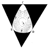
Figure 1:

Figure 2:

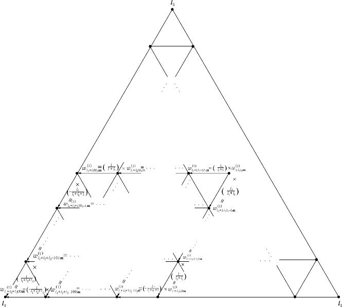
Figure 3:

References

- [1] V. A. Bogomolov. Dynamics of a Vorticity on a Sphere. Izv. Akad. Nauk SSSR, Mechanics of a Fluid and Gas, 1977, No. 6, P. 57-265.
- [2] J. J. Thomson. A Treatise on the Motion of Vortex Rings. London, MacMillan, 1883, P. 124.
- [3] H. Aref. On the Equilibrium and Stability of a Row of Point Vortices. J. Fluid Mech. 1995, V. 290, P. 167-2181.
- [4] L. G. Khazin. Regular Polygons of Point Vortices and Resonance Instability of Stationary States. Dokl. Akad. Nauk USSR, V. 230, 1976, No. 4, P. 799-2802.
- [5] A. V. Borisov, V. G. Lebedev. Dynamics of Three Vortices on a Plane and a Sphere — II. Regular and Chaotic Dynamics, V. 3, 1998, No. 2.
- [6] A. V. Borisov, I. S. Mamaev. Poisson Structures and Lie Algebras in Hamiltonian Mechanics. Izhevsk, editorial office of “Regular and Chaotic Dynamics”, 1999, P. 464.
- [7] V. V. Kozlov, S. D. Furta. Asymplotics of Solutions of Strongly Nonlinear Systems of Differential Equations. M., Izd. MGU, 1996.
- [8] A. P. Markeev. The Libration Points in Celestial Mechanics and Cosmic Dynamics. M., Nauka, 1978.