LIE ALGEBRAS IN VORTEX DYNAMICS AND
CELESTIAL MECHANICS — IV

1) Classificaton of the algebra of $n$ vortices on a plane
2) Solvable problems of vortex dynamics
3) Algebraization and reduction in a three-body problem

A. V. BOLSINOV
Faculty of Mechanics and Mathematics,
Department of Topology and Aplications
M. V. Lomonosov Moscow State University
Vorob’ievy Gory, Moscow, Russia, 119899
E-mail: bols@difgeo.math.msu.su
A. V. BORISOV
Faculty of Mechanics and Mathematics,
Department of Theoretical Mechanics Moscow State University
Vorob’ievy gory, 119899 Moscow, Russia
E-mail: borisov@uni.udm.ru
I. S. MAMAEV
Laboratory of Dynamical Chaos and Non Linearity,
Udmurt State University
Universitetskaya, 1, Izhevsk, Russia, 426034
E-mail: rcd@uni.udm.ru

Abstract

The work [13] introduces a naive description of dynamics of point vortices on a plane in terms of variables of distances and areas which generate Lie–Poisson structure. Using this approach a qualitative description of dynamics of point vortices on a plane and a sphere is obtained in the works [14, 15]. In this paper we consider more formal constructions of the general problem of $n$ vortices on a plane and a sphere. The developed methods of algebraization are also applied to the classical problem of the reduction in the three-body problem.

1 Classification of the algebra of $n$ vortices on a plane

1.1 Vortex algebra and Lie pencils

Let us introduce coordinates of vortices ${\bf r}_{k}(x_{k},y_{k}),\;k=1,\dots,n$ by complex variables $z_{k}=x_{k}+iy_{k},\;k=1,\ldots,n.$ The set ${\bf z}=(z_{1},\dots,z_{n})$ defines a vector in a complex linear space ${\mathbb{C}}^{n}$ with an Hermitian form

$$({\bf z,\bf w})_{\Gamma}=\sum_{i=1}^{n}\Gamma_{i}z_{i}\overline{w}_{i},\quad\Gamma_{i}\in{\mathbb{R}}\,,$$ (1)

where $\Gamma_{i}$ are vorticities.

The imaginary part of (1) gives the symplectic form corresponding to the Poisson bracket $\{x_{i},y_{j}\}=\frac{\delta_{ij}}{\Gamma_{i}}$. The Hamiltonian $\mathcal{H}$ and integrals of motion $P,\,Q,\,I$ of vortex system can be written as

$$\mathcal{H}=\frac{1}{16\pi}\sum\limits_{i,j=1}^{n}\Gamma_{i}\Gamma_{j}\ln|z_{i}-z_{j}|^{2}\,,$$ (2)

$$P+iQ=\sum\limits_{i=1}^{n}\Gamma_{i}z_{i}=({\bf z},{\bf z}_{0})_{\Gamma}\,,\qquad I=\sum\limits_{i=1}^{n}\Gamma_{i}|z_{i}|^{2}=({\bf z,z})_{\Gamma}\,,$$ (3)

here ${\bf z}_{0}=(1,1,\ldots,1)$ is a constant vector.

As relative variables we introduce the squares of mutual distances and doubled areas of triangles spanned on three vortices (see Fig. 1) as in [13]

$$\begin{array}[]{c}M_{lm}=({\bf r}_{i}-{\bf r}_{j})^{2}=(x_{i}-x_{j})^{2}+(y_{i}-y_{j})^{2},\\[8.0pt] \Delta_{ijk}=({\bf r}_{j}-{\bf r}_{i})\wedge({\bf r}_{k}-{\bf r}_{i})=(x_{j}-x_{i})(y_{k}-y_{i})-(x_{k}-x_{i})(y_{j}-y_{i}).\end{array}$$ (4)

New variables, as it was shown [13], generate a linear bracket, which also linearly depends on inverse intensities $1/\Gamma_{i}$

$$\{M_{ij},M_{kl}\}={} 4\Bigl{(}\frac{1}{\Gamma_{i}}\delta_{ik}-\frac{1}{\Gamma_{j}}\delta_{jk}\Bigr{)}\Delta_{ijl}+4\Bigl{(}\frac{1}{\Gamma_{i}}\delta_{il}-\frac{1}{\Gamma_{j}}\delta_{jl}\Bigr{)}\Delta_{ijk},$$

$$\{M_{ij},\Delta_{klm}\}={} \Bigl{(}\frac{1}{\Gamma_{i}}\delta_{ik}-\frac{1}{\Gamma_{j}}\delta_{jk}\Bigr{)}(M_{li}-M_{im}+M_{mj}-M_{jl})+$$

$$+\Bigl{(}\frac{1}{\Gamma_{i}}\delta_{il}-\frac{1}{\Gamma_{j}}\delta_{jl}\Bigr{)}(M_{mi}-M_{ik}+M_{kj}-M_{jm})+$$

$$+\Bigl{(}\frac{1}{\Gamma_{i}}\delta_{im}-\frac{1}{\Gamma_{j}}\delta_{jm}\Bigr{)}(M_{ki}-M_{il}+M_{lj}-M_{jk}),$$

$$\{\Delta_{ijk},\Delta_{lmn}\}={} \frac{\delta_{il}}{\Gamma_{i}}(\Delta_{jkn}-\Delta_{jkm})+\frac{\delta_{im}}{\Gamma_{i}}(\Delta_{jkl}-\Delta_{jkn})+{}$$ (5)

$$+\frac{\delta_{in}}{\Gamma_{i}}(\Delta_{jkm}-\Delta_{jkl})+\frac{\delta_{jl}}{\Gamma_{j}}(\Delta_{ikm}-\Delta_{ikn})+{}$$

$$+\frac{\delta_{jm}}{\Gamma_{j}}(\Delta_{ikn}-\Delta_{ikl})+\frac{\delta_{jn}}{\Gamma_{j}}(\Delta_{ikl}-\Delta_{ikm})+{}$$

$$+\frac{\delta_{kl}}{\Gamma_{k}}(\Delta_{ijn}-\Delta_{ijm})+\frac{\delta_{km}}{\Gamma_{k}}(\Delta_{ijl}-\Delta_{ijn})+\frac{\delta_{kn}}{\Gamma_{k}}(\Delta_{ijm}-\Delta_{ijl}).$$

Let us set invariant relations corresponding to real motions [13]

$$F_{ijkl}=\Delta_{ijk}+\Delta_{ikl}-\Delta_{lij}-\Delta_{ljk}=0\,,$$ (6)

$$F_{ijk}={(2\Delta_{ijk})}^{2}+M_{ij}^{2}+M_{jk}^{2}+M_{ik}^{2}-2(M_{ij}M_{jk}+M_{ij}M_{ik}+M_{jk}M_{ik})=0\,,$$ (7)

Relations (6) mean that the quadrangle spanned on the vortices $ijkl$ can be constructed of triangles by two ways (Fig. 1). Equations (7) are Heron formulas expressing the area of a triangle via its sides.

Let us note that for the structure (5) the Jacobi identity is fulfilled only on the submanifold defined by the first set of geometrical relations (6). Below, we consider the relations (6) to be fulfilled on default. Thus the brackets (5) define Lie–Poisson structure, which wee shall call vortex bracket.

The bracket (5) admits the linear Casimir function [13]

$$D=\sum_{i,j=1}^{N}\Gamma_{i}\Gamma_{j}M_{ij}=2\left(I\left(\sum\limits_{i=1}^{n}\Gamma_{i}\right)-Q^{2}-P^{2}\right)\,.$$ (8)

To define the real type of the corresponding Lie algebra we indicate an explicit isomorphism with some Lie pencil [10].

Remark 1. The compactness conditions of the real form (5), depending on intensities, imply that all mutual distances are bounded from above at any moment of time.

We consider a space of skew Hermitian $n\times n$ matrices and subspace $L$ in it generated by matrices of the form:

$$\begin{array}[]{c}\Delta_{lmk}=\begin{matrix}\mbox{}\\ l\\ \mbox{}\\ m\\ \mbox{}\\ k\\ \mbox{}\end{matrix}\left(\begin{array}[]{ccccccc}\ddots&&&&&&\\[-3.0pt] &0&&1&&-1&\\[-3.0pt] &&\ddots&&&&\\[-3.0pt] &-1&&0&&1&\\[-3.0pt] &&&&\ddots&&\\[-3.0pt] &1&&-1&&0&\\[-3.0pt] &&&&&&\ddots\end{array}\right),\\ M_{lm}=\begin{matrix}\mbox{}\\ l\\ \mbox{}\\ m\\ \mbox{}\end{matrix}\left(\begin{array}[]{ccccc}\ddots&&&&\\[-3.0pt] &i&&-i&\\[-3.0pt] &&\ddots&&\\[-3.0pt] &-i&&i&\\[-3.0pt] &&&&\ddots\end{array}\right).\end{array}$$ (9)

Let us describe the main properties of this subspace which can be verified by a straightforward calculation.

Proposition 1.

• The $L$ is a Lie subalgebra,

• This subalgebra is isomorphic to $u(n-1)$,

• The center of this subalgebra is generated by the element $\sum\limits_{m,l}M_{ml}$,

• The elements $\Delta_{lms}$ generate a subalgebra in $L$ isomorphic to $so(n-1)$,

• The following relation holds for any $k,l,m,s$:

  $$\Delta_{klm}+\Delta_{kms}+\Delta_{lks}+\Delta_{mls}=0,$$

• Commutation relations in $L$ coincide with the vortex bracket (5) for the case when all intensities are the same (and equal to unity).

Therefore, (9) determines an $n$-dimensional (unitary) linear representation of Lie algebra ${u(n-1)}$. There are no such irreducible representations, that is why it splits into a sum of the standard ${n-1}$-dimentional representation and one-dimensional trivial representation. This splitting is organized as follows.

Proposition 2. The representation space $V=\mathbb{C}^{n}$ splits into a direct sum of invariant subspaces $V=V_{1}\oplus V_{2}$, where $V_{1}={\mathbb{C}}^{n-1}$ is given by $z_{1}+z_{2}+\dots+z_{n}=0$ and a one-dimensional subspace $V_{2}={\mathbb{C}}$ is spanned on the vector ${\bf z}_{0}=(1,1,\dots,1)$.

Let us turn to the case of arbitrary intensities $\Gamma_{1},\dots,\Gamma_{n}.$ Consider the Lie pencil on the algebra of skew Hermitian $n\times n$ matrices generated by commutators

$$[X,Y]_{\Gamma^{-1}}=X\Gamma^{-1}Y-Y\Gamma^{-1}X,$$ (10)

where $\Gamma^{-1}$ is a real diagonal matrix of the form

$$\Gamma^{-1}=\left(\begin{matrix}\frac{1}{\Gamma_{1}}&&&\\ &\frac{1}{\Gamma_{2}}&&\\ &&\ddots&\\ &&&\frac{1}{\Gamma_{n}}\end{matrix}\right).$$ (11)

The remarkable fact is that the subalgebra $L$ is closed with respect to the commutator $[\cdot,\cdot]_{\Gamma^{-1}}$. Thus the family of commutators (10) generates some Lie pencil on $L$. Moreover, restricting the commutator $[\cdot,\cdot]_{\Gamma^{-1}}$ on $L$ we obtain the Lie algebra isomorphic to the vortex algebra $L_{\Gamma}$ corresponding to intensities $\Gamma_{1},\dots,\Gamma_{n}$. Thus one can deduce a symmetric isomorphism between the family of vortex algebras and a rather simple Lie pencil.

Using this construction we shall describe properties of vortex algebras.

Proposition 3. For positive $\Gamma_{i}$ the vortex algebra is isomorphic to ${u(n-1)}$.

Proof.

The corresponding isomorphism is constructed as follows. From the beginning let all intensities be equal to unity. All matrices (9) are skew Hermitian and satisfy the following property $A{\bf z}_{0}=0$, where ${\bf z}_{0}$ is the vector with coordinates  $(1,\,1,\,\ldots,\,1)$. In other words, this vector is invariant under the vortex algebra. Therefore its orthogonal completment, i. e., the hyperplane $V_{1}=\{{\bf z}\mid\sum z_{i}=0\}$ is also invariant.

We consider all skew Hermitian matrices possessing this property (that is, mapping ${\bf z}_{0}$ into zero) They form the subalgebra $u(n-1)$. Thus the vortex algebra in case of equal intensities is embedded into $u(n-1)$. But their dimensions coincide, therefore the algebras also coincide.

This can be shown more explicitly by choosing another basis in space $\mathbb{C}^{n}$. Consider a basis $\bf e_{1},\bf e_{2},\dots,\bf e_{n}$ where $\bf e_{1},\dots,\bf e_{n-1}$ is an orthonormal basis in the hyperplane $V_{1}$ (see Proposition 2) and ${\bf e}_{n}=(1/\sqrt{n},\dots,1/\sqrt{n})$. Rewriting matrices (9) from the vortex algebra in the new basis one can see that they take the form

$$\left(\begin{matrix}A_{n-1}&\begin{matrix}0\\ \vdots\\ 0\end{matrix}\\ \begin{matrix}0&\ldots&0\end{matrix}&0\end{matrix}\right),$$ (12)

where $A_{n-1}$ is a skew Hermitian $(n-1)\times(n-1)$ matrix. In this basis the isomorphism of the vortex algebra with $u(n-1)$ is evident. A defect of this basis is that this basis can’t be made symmetric with respect to all vortices.

Let us generalize these arguments to the case of arbitrary intensities. Transition to the new basis in ${\mathbb{C}}^{n}$ defines the conjugation of matrices in algebra (9) of the form $A=CA^{\prime}C^{-1}$, where $C$ is the transformation matrix. (In our case we can assume it to be real and orthogonal  $C^{-1}=C^{T}$). With this substitution the commutator of the vortex algebra transforms to the following form:

$$A\Gamma^{-1}B-B\Gamma^{-1}A =CA^{\prime}C^{-1}\Gamma^{-1}CB^{\prime}C^{-1}-CB^{\prime}C^{-1}\Gamma^{-1}CA^{\prime}C^{-1}=$$

$$=C[A^{\prime},B^{\prime}]_{\Gamma^{\prime}}C^{-1},$$

where

$$\Gamma^{\prime}=C^{-1}\Gamma^{-1}C=\left(\begin{matrix}\Gamma^{\prime}_{n-1}&\begin{matrix}\gamma_{1n}\\ \vdots\\ \gamma_{n-1,n}\end{matrix}\\ \begin{matrix}\gamma_{1n}&\ldots&\gamma_{n-1,n}\end{matrix}&\gamma_{n,n}\end{matrix}\right).$$

Here $\Gamma^{\prime}_{n-1}$ is the symmetric $(n-1)\times(n-1)$ matrix corresponding to the restriction of the form $\Gamma^{-1}$ onto the hyperplane $V_{1}$. This follows from the relation $C^{-1}=C^{T}$.

Taking into account that the last row and column of matrices $A$ and $B$ vanish one finds that the vortex commutator transforms to the form

$$[A^{\prime}_{n-1},B^{\prime}_{n-1}]_{\Gamma^{\prime}_{n-1}}.$$

Let us note that the matrix $\Gamma^{\prime}_{n-1}$ is positively defined and real, therefore one can take the root $(\Gamma^{\prime}_{n-1})^{1/2}$. Then the substitution

$$A^{\prime}_{n-1}=(\Gamma^{\prime}_{n-1})^{-1/2}A^{\prime\prime}_{n-1}(\Gamma^{\prime}_{n-1})^{-1/2}$$

reduces the commutator $[A^{\prime}_{n-1},B^{\prime}_{n-1}]_{\Gamma^{\prime}_{n-1}}$ to the standard one. The matrices remain skew Hermitian. This argument shows also that the vortex pencil under consideration is a subpencil of the standard pencil on the space of skew Hermitian matrices.$\blacksquare$

The main result following from this construction is that the properties of the vortex Lie algebra corresponding to parameters $\Gamma_{1},\dots,\Gamma_{n}$ are completely determined by properties of the bilinear form $\Gamma_{n-1}^{\prime}$. This form is the restriction of the form $\Gamma^{-1}$ onto the subspace $V_{1}=\{z_{1}+\dots+z_{N}=0\}$ (simply by the signature of this restriction).

Remark 2. Using the method of proof of Proposition 3 it is not difficult to show that in general case the vortex algebra is isomorphic to the algebra $u(p,q)$ with $p+q=n-1$.

Let us find conditions for which the algebra $L_{\Gamma}$ is compact, i. e., isomorphic to the Lie algebra $u(n-1)$. The necessary and sufficient condition is that $\Gamma_{n-1}^{\prime}$ is a form of fixed sign. In this case there are the following possibilities (we suppose that intensities are finite and differ from zero).

• The $\Gamma^{-1}$ is a form of fixed sign, i. e., all $\Gamma_{i}$ are simultaneously positive or negative.

• The form $\Gamma^{-1}$ has the signature $(n-1,1)$, all $\Gamma_{i}$ except for one are positive. Indeed the condition of positive definiteness of the restriction on $V_{1}$ requires that the form $\Gamma^{-1}$ is negative defined onto a one-dimensional orthogonal complement to the $V_{1}$ with respect to $\Gamma$ This condition is easy to find if one notices that the orthogonal complement to $V_{1}$ in the sense of (11) is a one dimensional subspace spanned on the vector $v_{\Gamma}=(\Gamma_{1},\dots,\Gamma_{n})$. It has the form

  $$(v_{\Gamma},v_{\Gamma})_{\Gamma^{-1}}=\sum\Gamma_{i}<0.$$

• Similarly, in the case of the signature $(1,n-1)$.

Finally we have the following

Proposition 4. The vortex Lie algebra $L_{\Gamma}$ is compact only in the following cases:

• All intensities have the same sign.

• All intensities except for one are positive and $\sum\limits_{i=1}^{n}\Gamma_{i}<0$.

• All intensities except for one are negative and $\sum\limits_{i=1}^{n}\Gamma_{i}>0$.

Remark 3. This proposition coincides with the one which was proved in the case of three vortices [14].

If the vortex algebra is not “semi-simple”, the conditions are defined similarly. It happens iff the form $\Gamma^{\prime}_{n-1}$ is degenerate on $V_{1}$. From linear algebra it follows that this condition equals to the requirement that the orthogonal complement to $V_{1}$ lies in $V_{1}$. It means that $v_{\Gamma}\in V_{1}$, i. e.

$$\Gamma_{1}+\ldots+\Gamma_{n}=0.$$

Let us note one more point. The subspace $\Delta\subset L$ spanned on vectors $\Delta_{lmn}$ is a subalgebra for any algebra of the pencil. Its compactness conditions are the same as those for the whole $L_{\Gamma}$, i. e., the form $\Gamma_{n-1}^{\prime}$ should be positive definite. Thus the vortex algebra $L_{\Gamma}$ is compact iff the subalgebra $\Delta$ is compact.

1.2 Reduction with symmetries and singular orbits

Now we explain the origin the nature of Lie pencils connected with the vortex algebra and describe the (singular) symplectic orbits of the algebra (5) corresponding to real motions. Consider a transition to relative variables (4) from the point of view of reduction with symmetries [22].

Hamiltonian function (2) and equations of motion of vortices are invariant under the action of the group $E(2)$. This action can be represented in the form

$$g\colon{\bf z}\to e^{i\varphi}{\bf z}+a{\bf z}_{0}\,,\quad g\in E(2)\,,$$ (13)

where ${\bf z}_{0}=(1,\,\ldots,\,1),\;a=a_{x}+ia_{y}$. Parameters $\varphi,\,a_{x},\,a_{y}$ define the translation and rotation corresponding to the element $g\in E(2)$.

The action (13) is the non-Hamiltonian group action [6]. Indeed integrals of motion (3) corresponding to translations $P,\,Q$ and to rotations $I$ form a Poisson structure that differs from Lie–Poisson structure of the algebra $e(2)$ by a constant, cocycle. Obviously this cocycle is unremovable and standard reduction with the momentum is impossible [6, 7, 22]. To execute the reduction in algebraic form we use the momentum map in some other way.

Consider the action of linear transformation preserving the form $(\cdot,\cdot)_{\Gamma}$ (1). The corresponding linear operators (matrices) form the group which is isomorphic to $U(p,q)$, $p+q=n$ and satisfies relations

$$X\Gamma X^{+}=\Gamma\,,\qquad\Gamma=\mbox{diag}(\Gamma_{1},\,\ldots,\,\Gamma_{n})\,.$$

Operators of the corresponding Lie algebra $A\in u(p,q)$ are defined by

$$A\Gamma+\Gamma A^{+}=0\,.$$ (14)

Since $\Gamma^{+}=\Gamma$ from (14), the matrix $A\Gamma$ is skew Hermitian. After the substitution $\phi(A)=A\Gamma$ the standard commutator transforms into the commutator $[\cdot,\cdot]_{\Gamma^{-1}}$ (10):

$$\phi([A,B])=[\phi(A),\phi(B)]_{\Gamma^{-1}}\,.$$

The advantage of this approach is that for any $\Gamma_{i}$ the algebra (14) is represented on the same space of skew Hermitian matrices. However, instead of the standard commutator it is necessary to use $[\cdot,\cdot]_{\Gamma^{-1}}$. In this case a family of Poisson brackets $\{\cdot,\cdot\}_{\Gamma^{-1}}$ appears on the corresponding coalgebra $u^{*}(p,q)$.

Linear vector fields corresponding to operators (14) in complex form can be written as

$$V_{A}=A{\bf z}=\phi(A)\Gamma^{-1}{\bf z}\,.$$

These fields are Hamiltonian [7] with

$$H_{A}=\frac{i}{2}(A{\bf z},{\bf z})_{\Gamma}=\frac{i}{2}\overline{{\bf z}}^{T}A\Gamma{\bf z}=\frac{i}{2}(\phi(A){\bf z},{\bf z})=\frac{i}{2}\overline{{\bf z}}^{T}\phi(A){\bf z}\,.$$ (15)

The bracket $\{\cdot,\cdot\}_{\Gamma^{-1}}$ of quadratic Hamiltonian functions is

$$\{H_{\phi(A)}({\bf z}),H_{\phi(B)}({\bf z})\}_{\Gamma^{-1}}=\frac{i}{2}\bigl{(}[\phi(A),\phi(B)]_{\Gamma^{-1}}{\bf z},{\bf z}\bigr{)},$$ (16)

and it corresponds to the commutator $[\cdot,\cdot]_{\Gamma^{-1}}$.

We can describe the momentum map $\mu({\bf z})$ explicitly using the standard identification $u(n)$ and $u^{*}(n)$ with the help of the form $\langle A,B\rangle=\mbox{Tr}AB$

$$\mbox{Tr}\mu({\bf z})\phi(A)=\mbox{Tr}\frac{i}{2}\overline{{\bf z}}^{T}\phi(A){\bf z}=\mbox{Tr}\left(\frac{i}{2}{\bf z}\overline{{\bf z}}^{T}\right)\phi(A).$$

Thus

$$\mu({\bf z})=\frac{i}{2}{\bf z}\overline{{\bf z}}^{T}=\frac{i}{2}\begin{pmatrix}z_{1}\overline{z}_{1}&\cdots&z_{1}\overline{z}_{n}\\ \vdots&\ddots&\vdots\\ z_{n}\overline{z}_{1}&\cdots&z_{n}\overline{z}_{n}\end{pmatrix}.$$ (17)

The formula (17) defines a map onto a singular symplectic orbit of the algebra $u(p,q)$ with the commutator $[\cdot,\cdot]_{\Gamma^{-1}}$. Now the integral (3) $I=\sum\Gamma_{i}z_{i}\overline{z}_{i}$ is a Casimir function, therefore the reduction with it is carried out. In case of all positive (negative) intensities the orbit is topologically homeomorphic to ${\mathbb{C}}P^{n-1}$, because under the map (17) all points of the form  $e^{i\varphi}{\bf z}$ (orbits of the rotation group action (11)) stick together.

Let us carry out the reduction with the remained integrals $P,Q$ (3) on the reduced space of matrices (17). Due to non-commutativity of $P,Q$ we can reduce only one degree of freedom [5]. The constant vector field corresponding to the translation in the direction $a=a_{x}+ia_{y}$ is generated by the linear Hamiltonian

$$H_{a}=({\bf z},\Gamma a{\bf z}_{0})=({\bf z},a{\bf z}_{0})_{\Gamma}\,.$$

It’s easy to show that Hamiltonians $H_{A}$ (15) commuting with $H_{a}$ are generated by matrices $A$ for which

$$A\Gamma{\bf z}_{0}=\phi(A){\bf z}_{0}=0\,.$$

So $\phi(A)$ belong to the subspace $L$ defined in the previous section (matrices (17) don’t belong to this space).

Now it is easy to see that squares of mutual distances and areas (4) also admit a natural representation of the form

$$M_{ij}(x,y) =|z_{i}-z_{j}|^{2}=i(M_{ij}{\bf z},{\bf z})\,,$$

$$\Delta_{ijk}(x,y) =i(\Delta_{ijk}{\bf z},{\bf z})\,,$$

where $M_{ij},\,\Delta_{ijk}$ are matrices (9). The momentum map $\mu({\bf z})$ into the corresponding algebra $u(p^{\prime},q^{\prime})$, $p^{\prime}+q^{\prime}=n-1$ has the form

$$\mu({\bf z})=\frac{i}{2}\left({\bf z}-\frac{({\bf z},{\bf z}_{0})\Gamma{\bf z}_{0}}{\sum\Gamma_{i}}\right)\left(\overline{\bf z}-\frac{({\bf z},{\bf z}_{0})\Gamma\overline{\bf z}_{0}}{\sum\Gamma_{i}}\right)^{T}\,.$$ (18)

Matrices (18) satisfy the relation $\mu({\bf z}){\bf z}_{0}=0$, i. e., they belong to the subspace $L$ defined in the previous section. In compact case the appropriate orbit is homeomorphic to ${\mathbb{C}}P^{n-2}$ and corresponds to the reduced phase space (after reducing two degrees of freedom). The rank of matrices (18) is equal to the unit. This is their characteristic property.

Remark 4. The structure and compactness conditions of the reduced phase space can be found by investigation (by methods of analytical geometry) of a common level surface of the first integrals (3). It is interesting that the algebraic approach also allows to solve this pure geometrical problem.

1.3 Symplectic coordinates

Let us describe an algorithm of construction of symplectic coordinates for the reduced system of $n$ vortices in the case of compact algebra $(u(n-1))$. The method of reduction of the vortex algebra (for this case) to the standard representation has been described above. In this case elements of the algebra are represented by skew Hermitian $(n-1)\times(n-1)$ matrices with an ordinary matrix commutator:

$$A=\begin{pmatrix}ih_{1}&x_{12}+iy_{12}&\cdots&x_{1,n-1}+iy_{1,n-1}\\ -x_{12}+iy_{12}&ih_{2}&\cdots&x_{2,n-1}+iy_{1,n-1}\\ {4}\\ -x_{1,n-1}+iy_{1,n-1}&-x_{2,n-1}+iy_{2,n-1}&\cdots&ih_{n-1}.\end{pmatrix}$$ (19)

Let us define a Poisson map ${\mathbb{R}}^{2(n-1)}\to u^{*}(n-1)$ onto a singular orbit $u^{*}(n-1)$ by formulas

$$\begin{aligned} h_{i}&=p_{i}\,,\\ x_{ij}&=\sqrt{h_{i}h_{j}}\sin(\varphi_{i}-\varphi_{j})\,,\\ y_{ij}&=\sqrt{h_{i}h_{j}}\cos(\varphi_{i}-\varphi_{j})\,,\end{aligned}\qquad i,\,j=1,\,\ldots,\,n-1\,.$$ (20)

The canonical bracket $\{\varphi_{i},p_{j}\}=\delta_{ij}$ turns in the standard Lie–Poisson bracket on $u^{*}(n-1)$. The orbit via variables $p_{i},\,\varphi_{i}$ is written as

$$p_{1}+p_{2}+\cdots+p_{n-1}=C=const\,.$$

This orbit is formed by matrices of rank 1 ($2\times 2$ minors equal zero). To introduce symplectic coordinates we carry out a symplectic transformation

$$r_{0} =p_{1}+p_{2}+\cdots+p_{n-1}\,,\quad s_{0} =\varphi_{1}\,,$$ (21)

$$r_{1} =p_{2}+\cdots+p_{n-1},\quad s_{1} =-\varphi_{1}+\varphi_{2}\,,$$

$$\vdots \vdots$$

$$r_{n-2} =p_{n-2}\,,\quad s_{n-2} =-\varphi_{n-1}+\varphi_{n-2}\,.$$

It is easy to see that the map (20) doesn’t depend on $s_{0}$, therefore $s_{1},\,\ldots,\,s_{n-2}$, $r_{1},\,\ldots,\,r_{n-2}$ define symplectic coordinates of $2(n-2)$-dimensional orbit $\mathbb{C}P^{n-2}$.

Remark 5. (Co)algebra $(u^{*})u(n-1)$ admits a linear change of variables $h_{i}\mapsto h_{i}+\lambda D,\;D=\sum\limits_{i=1}^{n-1}h_{i},\;\lambda=const$ preserving commutator relations. In this connection, the orbits given by matrices $F\in u(n)$ of rank 1 map into orbits for which the matrix $(A-\lambda D)$ has rank 1.

The orbit given by Heron relations (7) (in compact case) after the transition from variables $M,\triangle$ to standard variables of algebra $u(n-1)$ turns out among the above indicated orbits for some $\lambda$.

1.4 Canonical coordinates of a reduced four-vortex system. Poincaré section

Using the above described algorithm we shall point out canonical coordinates explicitly for a four-vortex problem of equal intensities.

Consider the coordinates on the algebra $u(3)$ corresponding to the matrix representation of the form (19)

$$A_{3}=\begin{pmatrix}ih_{1}&x_{3}+iy_{3}&-x_{2}+iy_{2}\\ -x_{3}+iy_{3}&ih_{2}&x_{1}+iy_{1}\\ x_{2}+iy_{2}&-x_{1}+iy_{1}&ih_{3},\\ \end{pmatrix}$$ (22)

In accordance with the above arguments these coordinates are expressed linearly via areas and squares of distances

$$x_{i}=\sum_{r}\delta^{r}_{(x_{i})}\Delta_{r}{(z)}\mbox{, }y_{i}=\sum_{k<l}m_{(y_{i})}^{kl}M_{kl}(z)\mbox{, }h_{i}=\sum_{k<l}m_{(h_{i})}^{kl}M_{kl}(z),\\ i=1,\dots,3\,.$$ (23)

To define coefficients $\delta_{(x_{i})}^{k},m_{(y_{i})}^{kl}m_{(h_{i})}^{kl}$ let us use the Proposition 3 and a matrix realization (9) of elements $\Delta_{r},M_{kl}$, where $\Delta_{1}=\Delta_{234}$, $\Delta_{2}=-\Delta_{134}$, $\Delta_{3}=\Delta_{124}$, $\Delta_{4}=-\Delta_{123}$. We choose the orthogonal matrix $C$, which reduces matrices of the vortex algebra (23) by the transformation $C^{T}AC$ to the form (12) as:

$$C=\begin{pmatrix}-\frac{1}{2}&-\frac{1}{2}&-\frac{1}{2}&\frac{1}{2}\\ \frac{1}{2}&\frac{1}{2}&-\frac{1}{2}&\frac{1}{2}\\ \frac{1}{2}&-\frac{1}{2}&\frac{1}{2}&\frac{1}{2}\\ -\frac{1}{2}&\frac{1}{2}&\frac{1}{2}&\frac{1}{2}\end{pmatrix}.$$ (24)

Let us set one of coordinates $h_{i},x_{i},y_{i}$ in the obtained matrix $A_{3}$ is equal to 1 and the others are equal to 0 and solve the system of linear equations. Thus we find corresponding coefficients $\delta_{(x_{i})}^{k},m_{(y_{i})}^{kl},m_{(h_{i})}^{kl}$. In this case

$$x_{1} =\frac{1}{4}(-\Delta_{1}+\Delta_{2}+\Delta_{3}-\Delta_{4})\mbox{, } x_{2} =\frac{1}{4}(-\Delta_{1}+\Delta_{2}-\Delta_{3}+\Delta_{4})\,,$$ (25)

$$x_{3} =\frac{1}{4}(-\Delta_{1}-\Delta_{2}+\Delta_{3}+\Delta_{4})\mbox{, } y_{1} =\frac{1}{4}(M_{14}-M_{23})\,,$$

$$y_{2} =\frac{1}{4}(M_{13}-M_{24})\mbox{, } y_{3} =\frac{1}{4}(M_{12}-M_{34})\,,$$

$$h_{1} =\frac{1}{4}(M_{12}+M_{34}+M_{13}+M_{24}-M_{14}-M_{23})\,,\hfil\hfil$$

$$h_{2} =\frac{1}{4}(M_{12}+M_{34}-M_{13}-M_{24}+M_{14}+M_{23})\,,\hfil\hfil$$

$$h_{3} =\frac{1}{4}(-M_{12}-M_{34}+M_{13}+M_{24}+M_{14}+M_{23})\,.\hfil\hfil$$

Denoting canonical coordinates (21) as $(g,G,h,H)$, we have

$$\begin{array}[]{c}\begin{aligned} x_{1}&=-\sqrt{(H-G)G}\sin g\mbox{, }&x_{2}&=\sqrt{(D-H)G}\sin(h+g)\,,\\[3.0pt] x_{3}&=-\sqrt{(D-H)(H-G)}\sin h\mbox{, }&y_{1}&=\sqrt{(H-G)G}\cos g\,,\\[3.0pt] y_{2}&=\sqrt{(D-H)G}\cos(h+g)\mbox{, }&y_{3}&=\sqrt{(D-H)(H-G)}\cos h\,,\end{aligned}\vskip 6.0pt plus 2.0pt minus 2.0pt\\ h_{1}=D-H,\qquad h_{2}=H-G,\qquad h_{3}=G,\end{array}$$ (26)

where $D=\frac{1}{4}\sum_{kl}M_{kl}$ is a constant of the Casimir function $u(3)$, in this connection $0<G<H<D$.

The Hamiltonian in new variables can be represented in the form

$${\cal H}={} \frac{1}{4\pi}\Bigl{\{}\ln\bigl{(}(D-G)^{2}-4(D-H)(H-G)\cos^{2}h\bigr{)}+{}$$ (27)

$$+\ln\bigl{(}(D-H+G)^{2}-4(D-H)G\cos^{2}(h+g)\bigr{)}+{}$$

$$+\ln\bigl{(}H^{2}-4(H-G)\cos^{2}g\bigr{)}\Bigr{\}}\,.$$

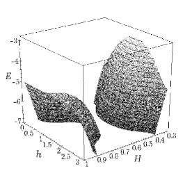
Figure 2: $G=0.3,\;g=\pi/2$

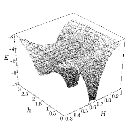
Figure 4: $G=0.3,\;g=0$

Let us construct the Poincaré map on a plane $(g,G)$ for different values of the energy $E={\cal H}(h,H,g,G)$. Surfaces of energy function in figures 2–4 for fixed ${g=g_{0}}$, ${G=G_{0}}$, $f(h,H)={\cal H}(h,H,g,G)$ show the complex structure of the isoenergetic surface.

We define an intersecting plane by the equation $H=H_{*}$. The value $H_{*}$ should be chosen so that $\forall g_{0},G_{0}<H_{*}$ equation $f(h,H_{*})=E$ has the unique solution with positive (negative) derivation $\frac{dH}{dt}$. As is obvious from the presented Fig. 2–4, that it is fulfilled not for all $H_{*}$ (analogous conditions for the intersecting plane $h=h_{*}$ are practically never fulfilled).

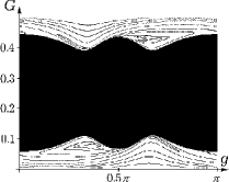
Figure 5: $H=0.5,\;E=-3.2$

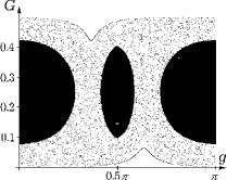
Figure 7: $H=0.5,\;E=-3.4$

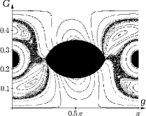
Figure 9: $H=0.5,\;E=-6.0$

The maximal possible energy $E_{T}=-4\ln 2\simeq-2.77\ldots$ corresponds to the Tompson configuration for $D=1$, in this connection $H=G=\frac{1}{2}$. In this case the phase portrait on a plane $(g,G)$ consists of the only line $G=\frac{1}{2}$. Phase portraits for the energies $E<E_{T}$ are represented in Fig. 5–10. Regions where the motion is impossible ($f(h,H_{*})=E$ has no solutions) corresponds to painted regions in Fig. 5–10. Figures show that with decreasing of the energy the stochastic layer increases first occupying all plane (Fig. 7, 8). Then it decreases and remains only near unstable solutions and separatrices (Fig. 9, 10). In the limit $E\to-\infty$ one of pairs of vortices merges and we obtain an integrable problem that is the system of three vortices.

1.5 Lax–Heisenberg representation

As a result of the reduction we can write equations of motion on the orbit of the coadjoint representation of the Lie algebra $u(p,q)$. This orbit is singular and consists of matrices of the form

$$L=\frac{i}{2}{\bf z\bar{\bf}z}^{\text{T}}\,,$$

where $\sum z_{i}=0$ (in a system connected with the center of vorticity).

According to a general principle (because of the simplicity of the corresponding Lie algebra [11]) we can rewrite equations in Lax–Heisenberg form:

$$\frac{dL}{dt}=[L,A]\,,$$

where $A=dH(L)$ is the differential of the Hamiltonian of the form

$$H(L)=\sum\Gamma_{i}\Gamma_{j}\log M_{ij}(L)\,.$$

Here $M_{ij}$ is interpreted as an element of the Lie algebra $u(n-1)$ and $M_{ij}(L)$  is a standard pairing between the algebra and coalgebra. In our case the identification $M_{ij}(L)=\pm\mbox{Tr}M_{ij}L=|z_{i}-z_{j}|^{2}$ is fulfilled.

The explicit form for the differential of the Hamiltonian is given by the formula:

$$dH(L)=\sum\Gamma_{i}\Gamma_{j}\frac{1}{M_{ij}(L)}M_{ij}\,,$$

i. e., $dH(L)$ is a linear combination of matrices $M_{ij}$. Thus the expression for the matrix  $A$ has the form

$$A=dH(L)=i\left(\begin{matrix}\sum_{j}\frac{\Gamma_{1}\Gamma_{j}}{|z_{1}-z_{j}|^{2}}&-\frac{\Gamma_{1}\Gamma_{2}}{|z_{1}-z_{2}|^{2}}&\ldots&-\frac{\Gamma_{1}\Gamma_{n}}{|z_{1}-z_{n}|^{2}}\\[5.0pt] -\frac{\Gamma_{2}\Gamma_{1}}{|z_{2}-z_{1}|^{2}}&\sum_{j}\frac{\Gamma_{2}\Gamma_{j}}{|z_{2}-z_{j}|^{2}}&\ldots&-\frac{\Gamma_{2}\Gamma_{n}}{|z_{2}-z_{n}|^{2}}\\[5.0pt] \vdots&\vdots&\ddots&\vdots\\ -\frac{\Gamma_{n}\Gamma_{1}}{|z_{n}-z_{1}|^{2}}&\ldots&-\frac{\Gamma_{n}\Gamma_{n-1}}{|z_{n}-z_{n-1}|^{2}}&\sum_{j}\frac{\Gamma_{n}\Gamma_{j}}{|z_{2}-z_{j}|^{2}}\end{matrix}\right).$$

If all intensities coincide with each other and equal to 1, the matrix $A$ is simplified:

$$A=i\left(\begin{matrix}\sum_{j}\frac{1}{|z_{1}-z_{j}|^{2}}&-\frac{1}{|z_{1}-z_{2}|^{2}}&\ldots&-\frac{1}{|z_{1}-z_{n}|^{2}}\\[5.0pt] -\frac{1}{|z_{2}-z_{1}|^{2}}&\sum_{j}\frac{1}{|z_{2}-z_{j}|^{2}}&\ldots&-\frac{1}{|z_{2}-z_{n}|^{2}}\\[5.0pt] \vdots&\vdots&\ddots&\vdots\\ -\frac{1}{|z_{n}-z_{1}|^{2}}&\ldots&-\frac{1}{|z_{n}-z_{n-1}|^{2}}&\sum_{j}\frac{1}{|z_{2}-z_{j}|^{2}}\end{matrix}\right).$$

In case of different intensities the additional procedure is required to reduce the commutator to the standard form.

1.6 Stationary configurations

In terms of $L-A$ pair the stationary configuration is naturally described. The stationary condition is equivalent to the fact that the matrices $L$ and $A$ commute: $[{L},{A}]=0$. In our case it means that

$$\frac{i}{2}A{\bf z}\bar{\bf z}^{\text{T}}=\frac{i}{2}{\bf z}\bar{\bf z}^{\text{T}}A=-\frac{i}{2}{\bf z}(\bar{A{\bf z}})^{\text{T}}.$$

Denoting ${\boldsymbol{b}}=A{\bf z}$, one has ${\boldsymbol{b}}\bar{\bf z}^{\text{T}}=-{\bf z}\bar{\boldsymbol{b}}^{\text{T}}$. It can be shown that it is possible only if $\boldsymbol{b}=i\lambda{\bf z}$, $\lambda\in\mathbb{R}$. It means that ${\bf z}$ is an eigenvector of a matrix $A$ (with an imaginary eigenvalue).

As a result we obtain a rather natural set of relations

$$\left(\begin{matrix}\sum_{j}\frac{1}{|z_{1}-z_{j}|^{2}}&-\frac{1}{|z_{1}-z_{2}|^{2}}&\ldots&-\frac{1}{|z_{1}-z_{n}|^{2}}\\ -\frac{1}{|z_{2}-z_{1}|^{2}}&\sum_{j}\frac{1}{|z_{2}-z_{j}|^{2}}&\ldots&-\frac{1}{|z_{2}-z_{n}|^{2}}\\ \vdots&\vdots&\ddots&\vdots\\ -\frac{1}{|z_{n}-z_{1}|^{2}}&\ldots&-\frac{1}{|z_{n}-z_{n-1}|^{2}}&\sum_{j}\frac{1}{|z_{2}-z_{j}|^{2}}\end{matrix}\right)\left(\begin{matrix}z_{1}\\ z_{2}\\ \vdots\\ z_{n}\end{matrix}\right)=\lambda\left(\begin{matrix}z_{1}\\ z_{2}\\ \vdots\\ z_{n}\end{matrix}\right).$$

This can be rewritten in a simpler form

$$\sum_{j}\frac{1}{z_{k}-z_{j}}=\lambda\bar{z}_{k}\mbox{, where }k=1,\dots,n.$$ (28)

Equations (28) can be obtained directly from the equations of motion under the condition that every point rotates around the origin with the same velocity $\lambda$.

Stationary configurations have been studied in several works (see [1, 16, 23]). Apparently new results can be obtained with the help of the following arguments.

• Stationary configurations can be interpreted as eigenvectors of a matrix $A$.

• Stationary configurations can be interpreted as singular points of Hamiltonian on an orbit (which is on $\mathbb{C}P^{n-1}$). As a Hamiltonian one can take a function $\tilde{H}=\prod_{k\neq j}|z_{k}-z_{j}|^{2}$. It is a positive function which vanishes on a submanifold of the “collapse”.

Using these arguments and by the investigation of a commutativity condition $[{L,A}]=0$, it would be interesting to give a theoretical explication of configurations from the “Los-Alamos” catalogue. For these configurations stable states of rotation realize on concentric circles (“atomic covers” by Kelvin) (see Fig. 11), where for the system of 11 vortices two possibilities $11=2+9$ or $11=3+8$) [2] are pointed out. As a rule these configurations possess the same type of symmetry (a rotational one or have a plane of symmetry). Recently in a short note in “Nature” [4] non-symmetric stationary configurations have been indicated for the vortex system of equal intensities.

Theoretically the simplest problem is to determine a number of collinear configurations in dependence on the ratio of intensities. In celestial mechanics (for positive masses $m_{i}$) the answer is given by the Multon theorem. In accordance with this theorem there is the only (rotating) collinear configuration for any permutation of masses $m_{1},\dots,m_{n}$ $(m_{i}>0)$ (the proof of this theorem is contained in [26]). For the three-vortex system the number of collinear configurations depends on the type of the algebra defined by Poisson brackets [14, 15]. Apparently there is such a connection in general case (for the system of $n$ vortices).

2 Solvable problems of vortex dynamics

In this section we consider in parallel the problems of dynamics of point vortices on a plane and sphere [9, 13]. The position of vortices on a sphere in the ”absolute” space is defined in cartesian ${\bf r}_{i}(x_{i},y_{i},z_{i})$ or spatial polar coordinates $(\theta_{i},\varphi_{i},\,i=1..N)$

$$x_{i}=R\sin\theta_{i}\cos\varphi_{i}\,,\qquad y_{i}=R\sin\theta_{i}\sin\varphi_{i}\,,\qquad z_{i}=R\cos\theta_{i}\,,$$

where $R$ is the radius of a sphere. Let us remind (see [13]), that the Hamiltonian function and Poisson bracket are defined by relations

$${}H=-\frac{1}{8\pi}\sum\limits_{i<j}\Gamma_{i}\Gamma_{j}\ln 4R^{2}\sin^{2}\frac{\theta_{ij}}{2}\,,$$

$${}\{\varphi_{i},\cos\theta_{j}\}=\frac{1}{R^{2}\Gamma_{i}}\delta_{ij}\,,\qquad i,j=1,\ldots,N\,,$$

where $\theta_{ij}$ is the angle between $i$-th and $j$-th vortices, and $\Gamma_{i}$ is a vortex intensity. For relative variables on a sphere the same labels — $M_{ij}$, $\Delta_{ijk}$ are used, however, their meaning is different, than for a plane [13]. So $M_{ij}$ is a length of a chord connecting the vortices, and $\Delta_{ijk}$ is equal to the ratio of volume of a tetrahedron spanned on three vortices and the center of a sphere to $\frac{1}{4}R$.

$$M_{ij}= {}(x_{i}-x_{j})^{2}+(y_{i}-y_{j})^{2}+(z_{i}-z_{j})^{2}\,,$$ (29)

$$\Delta_{ijk}= {}\frac{1}{R}({\bf r}_{i}{,\bf r}_{j}\times{\bf r}_{k})\,.$$

2.1 The particular case of the problem of $n$ vortices, the reduction to the problem of ${(n-1)}$ vortices

There is a special case of the problem of $n$ vortices on a plane and a sphere, for that case the problem can be reduced to the system of $(n-1)$ vortices with the same algebra of Poisson brackets, but reduced Hamiltonian function. The procedure of a reduction in Hamiltonian exposition corresponds to restriction of the system on a Poisson submanifold [18], which is defined in this case by involution conditions of integrals of motion. For vortices on a plane the integrals are given by relations (3), necessary conditions of reduction accept the form

$$\sum_{i=1}^{N}\Gamma_{i}=0\,,\quad Q=P=0\,.$$ (30)

For a sphere integrals of motion are obtained similarly:

$$\begin{gathered}F_{1}=R\sum_{i=1}^{N}\Gamma_{i}\sin\theta_{i}\cos\varphi_{i}\,,\quad F_{2}=R\sum_{i=1}^{N}\Gamma_{i}\sin\theta_{i}\sin\varphi_{i}\,,\quad F_{3}=R\sum_{i=1}^{N}\Gamma_{i}\cos\theta_{i}\,,\end{gathered}$$ (31)

and conditions of reduction

$$F_{1}=F_{2}=F_{3}=0\,.$$ (32)

Remark 6.The equations (30) have the following geometrical meaning: each vortex is situated at the center of vorticity of all remaining vortices. Really, expressing for example $\displaystyle\Gamma_{N}=-\sum_{i=1}^{N-1}\Gamma_{i}$ from (30), we have found that the absolute coordinates of the $N-$th vortex are defined by expressions

$${\bf r}_{N}=\frac{\sum\limits_{i=1}^{N-1}\Gamma_{i}{\bf r}_{i}}{\sum\limits_{i=1}^{N-1}\Gamma_{i}}\,.$$

The geometrical meaning of relations (32) on a sphere is a little different, it means, that the center of vorticity of a system of $n$ vortices coincides with the geometrical center of a sphere.

The mentioned below reduction happens because there is a possibility of calculation of positions of $n$ vortices basing on positions of $(n-1)$ vortices.

For a determination of additional invariant relations for relative variables we shall use identities [23]

$$\frac{1}{2}\sum_{k=1}^{N}\Gamma_{k}(M_{jk}-M_{ik})=P(x_{i}-x_{j})+Q(y_{i}-y_{j})$$ (33)

for plane which are fulfilled only under condition of $\displaystyle\smash{\sum_{i=1}^{N}}\Gamma_{i}=0$, that is also valid for the case of sphere [13]

$$\frac{1}{2}\sum_{k=1}^{N}\Gamma_{k}(M_{jk}-M_{ik})=R\bigl{(}F_{1}(x_{i}-x_{j})+F_{2}(y_{i}-y_{j})+F_{3}(z_{i}-z_{j})\bigr{)}\,.$$ (34)

Using conditions (30), (32), we have obtained $C_{N}^{2}$ invariant relations for $M_{ij}$

$$\sum_{k=1}^{N}\Gamma_{k}(M_{jk}-M_{ik})=0\,.$$ (35)

These relations we shall supplement by relations for $\Delta_{ijk}$, which also follow from (30), (32). It is possible to show by a straightforward calculation that the complete set of these relations determines a Poisson submanifold with the structure (5) and its generalization for a sphere [13].

Using representation for $M_{ij}$ in absolute coordinates (4) and (29), it is simple to verify that among the equations (35) only $n-1$ are linearly independent. Using these equations, we can express squares of distances from one of the vortices ($n$th vortex) to all the others $M_{kn},\;k=1,\ldots,n-1$ via mutual distances between $n-1$ vortices $M_{ij},\;i,j=1,\ldots,n-1$. Then substituting these expressions into initial Hamiltonian, we shall obtain a system with a bracket of the problem of $n-1$ vortices and reduced Hamiltonian function.

For the case of four vortices the explicit formulas of squares of distances from the first three vortices up to the fourth vortex $M_{14},M_{24},M_{34}$ have a form

$$\hookrightarrow M_{14}=\frac{\Gamma_{3}^{2}M_{13}+\Gamma_{2}^{2}M_{12}+\Gamma_{2}\Gamma_{3}(M_{12}-M_{23}+M_{13})}{(\Gamma_{1}+\Gamma_{2}+\Gamma_{3})^{2}}\,,$$ (36)

the reduced Hamiltonian is obtained by substitution (36) into initial Hamiltonian (2).

The system of three vortices is integrable (independently on a Hamiltonian given on algebra (5)), the described case corresponds to a special case of integrability of problem of four vortices (originating in work by Kirchhoff [21]). The phase portraits of this system at various intensities are presented in the previous work [15].

Remark 7. The indicated special cases of integrability correspond to a situation at which one of integrals reaches the extreme value. It is obvious, that in this case the system necessarily has additional invariant relations. For integrable systems that situation produces an additional degeneration. Delone case for Kovalevskaya top is one of examples. In this case the Kovalevskaya integral, which is the sum of two full squares will vanish, and the two-dimensional tori degenerate into one-dimensional torus(periodic and asymptotic solutions).

2.2 Particular solutions in the problem of four vortices

General equations of motion of vortices [13] with some restrictions on intensities $\Gamma_{i}$ allow a finite group of symmetries, the elements of the group are the permutations and reflections in some planes. Such discrete symmetries do not produce the general integrals of motion and do not allow reducing the order of a system. However, presence of these symmetries is connected to invariant submanifolds. The solution on that submanifolds can, as a rule, be obtained in quadratures [23].

Let us consider two problems of dynamics of four vortices on a plane and a sphere possessing two types of symmetry — central symmetry and reflection symmetry (for a plane, central symmetry and axial symmetry).

a. A centrally symmetric solution at $\bf{D=0}$. Equations of motion of four vortices on sphere (flat case is obtained with the passage to the limit $R\to\infty$) with condition $\Gamma_{1}=\Gamma_{3},$ $\Gamma_{2}=\Gamma_{4}$ allow invariant relations

$$\begin{array}[]{cc}M_{14}=M_{23}=M_{14}=M_{1}\,,&M_{12}=M_{34}=M_{3}\,,\\ \Delta_{234}=\Delta_{124}=\Delta_{1}\,,&\Delta_{213}=\Delta_{314}=\Delta_{2}\,.\end{array}$$ (37)

(The relations (37) don’t define the Poisson submanifold).

The equations (37) have the following geometrical meaning: a centrally symmetric configuration of vortices (the parallelogram), keeps this symmetry in all moments (see Fig. 12).

The analysis of a centrally symmetric solution in absolute variables through explicit quadratures is carried out by D. N. Goryachev [17] (see also [3]). However, he has not made clear the qualitative properties of motion and has introduced the very confusing classification. Let us introduce the qualitative analysis of relative motion.

The equations describing evolution of sides $M_{1},M_{3}$ and diagonals $M_{13}=M_{2}$, $M_{24}=M_{4}$ of the parallelogram, have a form

$$\begin{array}[]{l}\dot{M}_{1}=4\Gamma_{1}\Delta_{2}\left(\frac{1}{M_{2}}-\frac{1}{M_{3}}\right)+4\Gamma_{2}\Delta_{1}\left(\frac{1}{M_{4}}-\frac{1}{M_{3}}\right)\,,\\[10.0pt] \dot{M}_{3}=4\Gamma_{1}\Delta_{2}\left(\frac{1}{M_{1}}-\frac{1}{M_{2}}\right)+4\Gamma_{2}\Delta_{1}\left(\frac{1}{M_{1}}-\frac{1}{M_{4}}\right)\,,\\[10.0pt] \dot{M}_{2}=8\Gamma_{2}\Delta_{2}\left(\frac{1}{M_{3}}-\frac{1}{M_{1}}\right)\,,\\[10.0pt] \dot{M}_{4}=8\Gamma_{1}\Delta_{1}\left(\frac{1}{M_{3}}-\frac{1}{M_{1}}\right)\,.\end{array}$$ (38)

For a sphere (for a plane $R\to\infty$) the geometrical relations between $M,\Delta$ can be written as

$$\begin{array}[]{l}\Delta_{1}\left(4R^{2}-M_{2}\right)+\Delta_{2}\left(4R^{2}-M_{1}-M_{3}\right)=0\,,\\[6.0pt] \Delta_{1}\left(4R^{2}-M_{1}-M_{3}\right)+\Delta_{2}\left(4R^{2}-M_{4}\right)=0\,.\\[6.0pt] \end{array}$$ (39)

System (39) is solvable with respect to $\Delta_{1},\Delta_{2}$ under condition of

$$2(M_{1}+M_{3})-(M_{2}+M_{4})+\frac{1}{4R^{2}}\left(M_{2}M_{4}-(M_{1}+M_{3})^{2}\right)=0\,.$$ (40)

The linear integral of the equations (38) corresponding to the Casimir function (8) has a form

$$D=2\Gamma_{1}\Gamma_{2}(M_{1}+M_{3})+\Gamma_{1}^{2}M_{2}+\Gamma_{2}^{2}M_{4}\,.$$ (41)

With the help of relations (39) and regularization of time, the system (38) can be reduced to two inhomogeneous equations describing evolution of sides of the parallelogram $M_{1},\,M_{3}$.

For simplicity we consider the limited case $D=0$, that is also a necessary condition of a collapse [24]. Geometrical interpretations on a plane and a sphere are a little different, therefore we shall consider these cases separately.

1) P l a n e.

Relations (39),(40) for a plane ($R\to\infty$) have a form

$$\begin{array}[]{c}\Delta_{1}=-\Delta_{2}=\Delta\,,\\[6.0pt] 2(M_{1}+M_{3})-(M_{2}+M_{4})=0\,.\end{array}$$ (42)

Taking into account, that in (41) $D=0$, we found the equation, describing a trajectory of system on plane $M_{1},M_{3}$ (sides of a parallelogram)

$$\frac{dM_{1}}{dM_{3}}=-\frac{M_{1}\left(2\Gamma_{1}\Gamma_{2}(M_{1}+M_{3})+(\Gamma_{1}^{2}+\Gamma_{2}^{2})M_{3}\right)}{M_{3}\left(2\Gamma_{1}\Gamma_{2}(M_{1}+M_{3})+(\Gamma_{1}^{2}+\Gamma_{2}^{2})M_{1}\right)}\,.$$ (43)

The solution of this equation has a form

$$\begin{array}[]{c}\left(M_{1}-M_{3}\right)^{2}=\left(M_{1}+M_{3}\right)^{2}-C\left(M_{1}+M_{3}\right)^{-2\alpha}\,,\\[6.0pt] \alpha=\frac{\Gamma_{1}^{2}+\Gamma_{2}^{2}}{4\Gamma_{1}\Gamma_{2}}\,,\qquad C=const\,.\end{array}$$ (44)

(Index $\alpha<0$, because with $D=0$ intensities $\Gamma_{1},\Gamma_{2}$ have different signs).

In a quadrant $M_{1}>0,\,M_{2}>0$ (which corresponds to physical area) three types of trajectories (44) are possible depending on $\alpha$:

• $-1<\alpha<0$ — all trajectories are closed, started from the origin of coordinates, tangenting axes $OM_{1}$ $OM_{2}$ (see. Fig. 13, a), a) (inhomogeneous collapse).

• $\alpha<-1$ — all trajectory are curves asymptotically approaching to coordinate axes (see Fig. 13,b).

• $\alpha=-1$ — all trajectories are straight lines moving through the origin of coordinates (see Fig. 13,c) (homogeneous collapse) [24].

The physical area on a plane $M_{1},M_{3}$ is defined by the part of a positive quadrant $(M_{1}>0$, ${M_{3}>0)}$, for which the inequality $\Delta^{2}>0$ is fulfilled. When the trajectory reached a boundary ${\Delta^{2}=0}$, the sign in the equation (43) should be changed (reflection) that corresponds to the same trajectory passing in the opposite direction. It is easy to show, that the equation $\Delta^{2}=0$ is defined by two straight lines on a plane $M_{1},M_{3}$, which are situated inside a quadrant   $M_{1}>0,\,M_{3}>0$ for any intensities $\Gamma_{1},\Gamma_{2}$. Hence, except for a case $3^{\circ}$ vortices are moving in the bounded area without collisions and scattering. In the system in case $3^{\circ}$ the homogeneous collapse of all vortices or homogeneous scattering happen.

For the problem on a plane each point of the trajectory on the plane $M_{1},M_{3}$ correspond to two configurations of vortices, which differ only by permutation: $1\leftrightarrow 3$, or $2\leftrightarrow 4$ (see Fig. 12).

Remark 8. The condition of a homogeneous collapse ($\alpha=-1$) from the analysis of motion in absolute variables is obtained in [24]. As result of quasi-homogeneity of the equations the condition of a homogeneous collapse can be obtained by investigation of existence conditions of solutions of the form $M_{i}=C_{i}t^{\xi},\,C_{i}=const$ of the system.

Remark 9. For a plane the system (38) with a regularization

$$d\tau=\frac{4\Delta}{M_{1}M_{2}M_{3}M_{4}}\,dt$$

can be reduced to a homogeneous Hamiltonian system

$$\frac{dM_{1}}{d\tau} =\Gamma_{1}M_{1}M_{4}(M_{3}-M_{2})+\Gamma_{2}M_{1}M_{2}(M_{4}-M_{3})\,,$$ (45)

$$\frac{dM_{3}}{d\tau} =\Gamma_{1}M_{3}M_{4}(M_{2}-M_{1})+\Gamma_{2}M_{2}M_{3}(M_{1}-M_{3})\,,$$ (46)

$$\frac{dM_{2}}{d\tau} =2\Gamma_{2}M_{2}M_{4}(M_{1}-M_{3})\,,$$ (47)

$$\frac{dM_{4}}{d\tau} =2\Gamma_{1}M_{2}M_{4}(M_{3}-M_{1})$$ (48)

with a Poisson bracket of the form

$$\{M_{1},M_{2}\} =\frac{1}{\Gamma_{1}}M_{1}M_{2}M_{3}M_{4}\,,\quad \{M_{1},M_{3}\} =\frac{1}{2}\left(\frac{1}{\Gamma_{1}}-\frac{1}{\Gamma_{2}}\right)M_{1}M_{2}M_{3}M_{4}\,,$$

$$\{M_{2},M_{3}\} =\frac{1}{\Gamma_{1}}M_{1}M_{2}M_{3}M_{4}\,,\quad \{M_{1},M_{4}\} =-\frac{1}{\Gamma_{2}}M_{1}M_{2}M_{3}M_{4}\,,$$ (49)

$$\{M_{2},M_{4}\} =0,\quad \{M_{3},M_{4}\} =\frac{1}{\Gamma_{2}}M_{1}M_{2}M_{3}M_{4}$$

and Hamiltonian

$$H=2\Gamma_{1}\Gamma_{2}\ln M_{1}+\Gamma_{1}^{2}\ln M_{2}+2\Gamma_{1}\Gamma_{2}\ln M_{3}+\Gamma_{2}^{2}\ln M_{4}\,.$$

The rank of a bracket (49) is equal to two, hence dividing the bracket on $M_{1}M_{2}M_{3}M_{4}$, it can be reduced to a constant without violation of the Jacobi identity.

2) S p h e r e.

For a centrally symmetric configuration on a sphere we also consider a projection of trajectories to a plane $M_{1},M_{3}$ (see Fig. 14). The form of physical area defined by inequalities $\Delta_{i}^{2}>0,\,i=1,2$ varies. Moreover, there are two differences from a case of plane connected with the nonlinearity of the equation (40). At first, each point $M_{1},M_{3}$ correspond to two solutions of the equation (40), and therefore two various (spatial) parallelograms with the given sides on a sphere, these parallelograms are not reduced to each other by permutation $1\leftrightarrow 3\;(2\leftrightarrow 4)$. Secondly, the system (38) is not reduced to two quasi-homogeneous equations.

Let us express $\Delta_{1}$ and $\Delta_{2}$ from (39) with preservation of homogeneity

$$\Delta_{1}=(M_{4}-M_{1}-M_{3})\Delta\,,\qquad\Delta_{2}=(M_{2}-M_{1}-M_{3})\Delta\,.$$ (50)

Also we shall make change of the time

$$dt=\smash{\frac{4\Delta}{M_{1}M_{3}}}\,d\tau\,.$$

So we obtained the system describing evolution of variables $M_{1}$, $M_{2}$, $M_{3}$, $M_{4}$

$$M^{\prime}_{1} =M_{1}\left(\Gamma_{1}\frac{(M_{2}-M_{1}-M_{3})(M_{3}-M_{2})}{M_{2}}+\Gamma_{2}\frac{(M_{4}-M_{1}-M_{3})(M_{3}-M_{4})}{M_{4}}\right)\,,$$ (51)

$$M^{\prime}_{3} =M_{3}\left(\Gamma_{1}\frac{(M_{2}-M_{1}-M_{3})(M_{2}-M_{1})}{M_{2}}+\Gamma_{2}\frac{(M_{4}-M_{1}-M_{3})(M_{4}-M_{1})}{M_{4}}\right)\,,$$

$$M^{\prime}_{2} =2\Gamma_{2}(M_{2}-M_{1}-M_{3})(M_{1}-M_{3})\,,$$

$$M^{\prime}_{4} =2\Gamma_{1}(M_{4}-M_{1}-M_{3})(M_{1}-M_{3})\,,$$

here primes denote derivation on new time $\tau$.

Let us introduce a linear change of variables reducing system (51) to two differential equations, which has the most simple form.

Let us choose variables $x,y,M,N$:

$$x =\Gamma_{1}M_{2}+\Gamma_{2}M_{4}\,,\qquad y =\Gamma_{1}^{2}M_{2}-\Gamma_{2}^{2}M_{4}\,,$$ (52)

$$M =M_{1}+M_{3}\,,\qquad N =M_{1}-M_{3}\,.$$

With the help of a relation (41) where $D=0$ and (40) which have a form

$$x=-{\frac{y^{2}}{16R^{2}\Gamma_{1}\Gamma_{2}(\Gamma_{1}+\Gamma_{2})}}\,,$$ (53)

we exclude $x,M$ from (51). In outcome we obtain the equations of evolution $y,N$

$$\frac{dy}{d\tau}= \,4(\Gamma_{1}+\Gamma_{2})yN\,,$$

$$\frac{dN}{d\tau}= -\frac{1}{4(\Gamma_{1}+\Gamma_{2})^{3}\Gamma_{1}^{2}\Gamma_{2}^{2}}\biggl{[}\frac{2ky-\Gamma_{1}(\Gamma_{1}+\Gamma_{2})}{\Gamma_{2}(ky-\Gamma_{1}(\Gamma_{1}+\Gamma_{2}))}\Bigl{(}4\Gamma_{1}^{3}\Gamma_{2}^{2}(\Gamma_{1}+\Gamma_{2})^{4}N^{2}-$$

$$-y^{2}(2ky-\Gamma_{1}^{2}+\Gamma_{2}^{2})(2ky(\Gamma_{1}+2\Gamma_{2})-\Gamma_{1}(\Gamma_{1}+3\Gamma_{2})(\Gamma_{1}+\Gamma_{2}))\Bigr{)}+$$

$$+\frac{2ky+\Gamma_{2}(\Gamma_{1}+\Gamma_{2})}{\Gamma_{1}(ky+\Gamma_{2}(\Gamma_{1}+\Gamma_{2}))}\Bigl{(}4\Gamma_{1}^{2}\Gamma_{2}^{3}(\Gamma_{1}+\Gamma_{2})^{4}N^{2}-$$ (54)

$$-y^{2}(2ky-\Gamma_{1}^{2}+\Gamma_{2}^{2})(2ky(\Gamma_{2}+2\Gamma_{1})+\Gamma_{2}(\Gamma_{2}+3\Gamma_{1})(\Gamma_{1}+\Gamma_{2}))\Bigr{)}\biggr{]}\,.$$

hereinafter $k=1/R^{2}$.

The projection of trajectory $y(\tau),\,N(\tau)$ on the plane $M_{1},M_{3}$ is defined by the formulas $M_{1}=\frac{1}{2}(M+N),M_{3}=\frac{1}{2}(M-N)$, where

$$M=\frac{\Gamma_{2}-\Gamma_{1}}{2\Gamma_{1}\Gamma_{2}(\Gamma_{1}+\Gamma_{2})}y+\frac{y^{2}}{16R^{2}\Gamma_{1}\Gamma_{2}(\Gamma_{1}+\Gamma_{2})^{2}}\,,\qquad(\Gamma_{1}\Gamma_{2}<0)\,.$$ (55)

The equation (55) allows real solutions only for $M\leq M_{max}=-\frac{(\Gamma_{1}-\Gamma_{2})^{2}}{\Gamma_{1}\Gamma_{2}}R^{2}.$ Therefore, in case of a sphere the physically accessible area on a plane is defined by inequalities

$$M_{1}+M_{3}\leq M_{max}\,,$$ (56)

$$\begin{aligned} 4\Delta_{1}^{2}=&\,2(M_{1}M_{4}+M_{3}M_{4}+M_{1}M_{3})-M_{1}^{2}-M_{3}^{2}-M_{4}^{2}-\frac{1}{R^{2}}M_{1}M_{3}M_{4}\geq 0\,,\\ 4\Delta_{2}^{2}=&\,2(M_{1}M_{2}+M_{3}M_{2}+M_{1}M_{3})-M_{1}^{2}-M_{3}^{2}-M_{2}^{2}-\frac{1}{R^{2}}M_{1}M_{3}M_{2}\geq 0\,.\end{aligned}$$ (57)

In the area (57) the equation (55) has two roots, therefore we have on a plane $M_{1},M_{3}$ a projection of two different areas of possible positions of vortices defined by inequalities (56) and equations (55). If the areas (56) do not reach a straight line $M_{1}+M_{3}=M_{max}$ (Fig. 14 b, c), the point, beginning to move inside one area, remains there in all moments. When the point reached boundaries ($\Delta_{i}=0$), it is necessary to change a sign of time, and the trajectory is passed in the opposite direction. In a case when the straight line $M_{1}+M_{3}=M_{max}$ passes through the interior of areas (56) (Fig. 14 a) the trajectory, that had reached that line, passes from one area in another and is described by other solution of the equation (55). Characteristics of phase portraits in case of a sphere is the occurrence new motionless points, absent in a flat case. If the second necessary condition of a collapse is realized ($\Gamma_{1}^{2}+\Gamma_{2}^{2}=-4\Gamma_{1}\Gamma_{1}$), we can see on a Fig. 14 c), that some of trajectories starting at the origin of coordinates goes to origin again and do not reach the boundary of area (collinear positions) and some trajectories goes back to origin only after the reaching of boundary. It means, that the collapse remains homogeneous only near the origin of coordinates.

b. A reflective-symmetric solution. For a system of two cooperating vortex pairs $\Gamma_{1}=-\Gamma_{4}$, ${\Gamma_{2}=-\Gamma_{3}}$ the general system of four vortices on a sphere and on a plane also allows invariant relations

$$\begin{array}[]{cc}M_{12}=M_{34}=M_{1}\,,&M_{13}=M_{24}=M_{3}\,,\\[5.0pt] \Delta_{123}=\Delta_{234}=\Delta_{1}\,,&\Delta_{124}=\Delta_{134}=\Delta_{2}\,.\end{array}$$ (58)

These equations have the following geometrical meaning. The vortices located at the initial momentum in tops of a trapezoid will form a trapezoid during all time of motion (see Fig. 15) [23]. The given configuration has a reflection (axial) symmetry. The equations describing the evolution of sides and diagonals of a trapezoid have a form

$$\dot{M}_{1} =4\Gamma_{2}\Delta_{1}\left(\frac{1}{M_{4}}-\frac{1}{M_{3}}\right)+4\Gamma_{1}\Delta_{2}\left(\frac{1}{M_{2}}-\frac{1}{M_{3}}\right)\,,$$ (59)

$$\dot{M}_{3} =4\Gamma_{2}\Delta_{1}\left(\frac{1}{M_{4}}-\frac{1}{M_{1}}\right)+4\Gamma_{2}\Delta_{2}\left(\frac{1}{M_{2}}-\frac{1}{M_{1}}\right)\,,$$

$$\dot{M}_{2} =8\Gamma_{2}\Delta_{2}\left(\frac{1}{M_{1}}-\frac{1}{M_{3}}\right)\,,$$

$$\dot{M}_{4} =8\Gamma_{1}\Delta_{1}\left(\frac{1}{M_{1}}-\frac{1}{M_{3}}\right)\,.$$

Here $M_{2}=M_{14},\;M_{4}=M_{23}$ — of the bases of a trapezoid.

The geometrical relations between $M,\,\Delta$ in this case have the identical form on a plane and sphere:

$$\Delta_{1}M_{4}+\Delta_{2}(M_{3}-M_{1}) =0\,,$$ (60)

$$\Delta_{1}(M_{3}-M_{1})+\Delta_{2}M_{2} =0\,,$$

the condition of their resolvability with respect to $\Delta_{1},\,\Delta_{2}$ has a form

$$M_{2}M_{4}-(M_{1}-M_{3})^{2}=0\,.$$ (61)

The integral of the momentum has a form

$$D=2\Gamma_{1}\Gamma_{2}(M_{1}-M_{3})-\Gamma_{1}^{2}M_{4}-\Gamma_{2}^{2}M_{2}\,.$$ (62)

From the equations (59–61) it follows that trajectories of a system in space $M_{1},M_{2},M_{3},M_{4}$ coincide for cases of a plane and sphere. The difference between these problems consists in form of physical areas defined by inequalities (56).

With the help of the equations (60) we shall express $\Delta_{1},\Delta_{2}$ by

$$\Delta_{1}=(M_{2}-M_{1}+M_{3})\Delta,\quad\Delta_{2}=-(M_{4}-M_{1}+M_{3})\Delta\,,$$

and also we shall exclude $\Delta$ with the help of regularizing substitution of time

$$dt=\frac{4\Delta}{M_{1}M_{3}}d\tau\,.$$

To reduce the regularized equation to the system of two equations, we make the substitution (52). As a result of the existence of an integral of the moment between the variables $x,y$ the following relation is fulfilled

$$\frac{4\Gamma_{1}\Gamma_{2}}{\Gamma_{1}+\Gamma_{2}}Dx+y^{2}+\frac{2(\Gamma_{1}\Gamma_{2})}{\Gamma_{1}+\Gamma_{2}}Dy+D^{2}=0\,.$$ (63)

Using (63) and equation (61), we find

$$N=-\frac{y^{2}}{4\Gamma_{1}\Gamma_{2}D}+\frac{D}{4\Gamma_{1}\Gamma_{2}}\,.$$ (64)

With $D\neq 0$ from relations (62), (63) and (64) all $M_{1},M_{2},M_{3},M_{4}$ can be expressed through $M,y$. For the variables $M,y$ we shall get the equations of the form

$$\begin{array}[]{c}\frac{dy}{d\tau}=\frac{(y^{2}-D^{2})(y(\Gamma_{1}+\Gamma_{2})+D(\Gamma_{1}-\Gamma_{2}))}{4\Gamma_{1}\Gamma_{2}D}\,,\\[12.0pt] \begin{aligned} \frac{dM}{d\tau}=&\,\frac{1}{32D^{2}\Gamma_{1}\Gamma_{2}^{3}(D-y)}\left[D(\Gamma_{2}-\Gamma_{1})-y(\Gamma_{2}+\Gamma_{1})\bigr{)}\bigl{(}16D^{2}\Gamma_{1}^{2}\Gamma_{2}^{2}M^{2}+\right.\\[5.0pt] &\left.+8(D-y)^{2}D\Gamma_{2}^{2}M-(D^{2}-y^{2})^{2}\right]-\\[10.0pt] &-\frac{1}{32D^{2}\Gamma_{1}^{3}\Gamma_{2}(D+y)}\left[D(\Gamma_{2}-\Gamma_{1})-y(\Gamma_{2}+\Gamma_{1}))(16D^{2}\Gamma_{1}^{2}\Gamma_{2}^{2}M_{2}+\right.\\[5.0pt] &\left.+8(D+y)^{2}D\Gamma_{1}^{2}M-(D^{2}-y^{2})^{2}\right]\,.\end{aligned}\end{array}$$ (65)

By analogy with a centrally symmetric solution, we shall consider a projection of a trajectory to a plane $M_{1},M_{3}$. Besides inequalities (56) the physical area is defined by an additional condition (corollary of the relation (64))

$$D(D-4\Gamma_{1}\Gamma_{2}N)>0\,.$$ (66)

Two various points of a phase space (two solutions of the equation (64)) are projected in each point on a plane $M_{1},M_{3}$, satisfying to inequalities (56), (66). It is more evident if we imagine that two different areas defined by an inequality (56) are glued together along a line $M_{1}-M_{3}=N_{0}$. When a point reached a boundary $\Delta_{i}=0$, it is reflected back and moves on the same trajectory, and at reaching boundary (66) the point passes from one area to another (see. Fig. 16 a, 16 b). In figures for convenience we have unrolled the areas, which have been glued together along a line $M_{1}-M_{3}=N_{0}$, where $N_{0}$ is a solution of the equation $D-4\Gamma_{1}\Gamma_{2}N_{0}=0$. The difference of a plane from a sphere is exhibited in form of physical areas. For a plane (see Fig. 16 a) two types of trajectories exist:

1. Trajectories are touched once boundaries $\Delta_{i}=0$ and then leaving to infinity;

2. Trajectories stayed between boundaries $\Delta_{i}=0$.

Different motions of vortices correspond to these cases: in the first case the vortices run up, passing only once through a collinear configuration, in second case vortex pairs alternately pass one through another (leapfrog of Helmholtz), remaining on bounded distance. Only trajectories of the second type exists for a sphere. The analysis of leapfrog on a plane was carried out by other method in [23].

Let us introduce also, for completeness, the equation of motion and geometrical interpretation at the zero moment $D=0$ (necessary condition of a collapse [24]).

According to (63) in this case $y=0$, and all mutual distances $M_{1},\dots,M_{4}$ can be expressed via variables $x,M$ by formulas

$$\begin{array}[]{c}M_{2}=\frac{\Gamma_{2}x}{\Gamma_{1}(\Gamma_{1}+\Gamma_{2})}\,,\quad M_{4}=\frac{\Gamma_{1}x}{\Gamma_{2}(\Gamma_{1}+\Gamma_{2})},\quad N=\frac{x}{\Gamma_{1}+\Gamma_{2}}\,,\\[10.0pt] M_{1}=\frac{1}{2}(M+N),\quad M_{3}=\frac{1}{2}(M-N)\,.\end{array}$$

The equations of motion for $m=(\Gamma_{1}+\Gamma_{2})M$ and $x$ have a form

$$\frac{dx}{d\tau} =-2x^{2}\,,$$ (67)

$$\frac{dm}{d\tau} =\frac{1}{2}\left(\frac{\Gamma_{1}}{\Gamma_{2}}+\frac{\Gamma_{2}}{\Gamma_{1}}\right)m^{2}-2xm-\frac{1}{2}\left(\frac{\Gamma_{1}}{\Gamma_{2}}+\frac{\Gamma_{2}}{\Gamma_{1}}\right)x^{2}\,.$$

The trajectory, defined by the system (67), is obtained from equation

$$m=x\frac{Cx^{4/a}-1}{Cx^{4/a}-1}\,,\quad a=\frac{1}{2}\left(\frac{\Gamma_{1}}{\Gamma_{2}}+\frac{\Gamma_{2}}{\Gamma_{1}}\right)\,,$$ (68)

where $C$ is a constant of an integration. The equation, defining the form of area $(\Delta_{i}>0)$ on a plane $m,x$ has a form

$$\Gamma_{1}\Gamma_{2}\left(x(m-ax)-\frac{(m^{2}-x^{2})x}{8R^{2}(\Gamma_{1}+\Gamma_{2})^{2}}\right)>0\,.$$ (69)

Analyzing (68), (69) near to the origin of coordinates $m=x=0$ it is possible to conclude that for reflectional symmetrical solution the simultaneous collapse of four vortices is impossible.

The discussed above integrable systems of vortex dynamics allow the complete enough analysis with the help of qualitative research of dynamical systems on a plane. At the same time application of classical methods of an explicit solution with the help of the theory of special (Abelian) functions produces very bulky expressions, and that expressions are not permitting to make any of representation about the real motion [17].

3 Algebraization and reduction of the three-body problem

The reduction in the three-body problem of celestial mechanics is for the first time systematically considered in the lectures of Jacobi  [19]. He dwelt upon barycentric coordinates, which permit to ignore uniform motion of the centre of masses, and also to the procedure of elimination of momentum (elimination of a knot). Constructively this process reducing in a plane (spatial) case in a system with three (four) degrees of freedom was executed by Radout, Brunce, Charlier, Lie, Levi-Chevita and Whittaker, the review of their researches contains in the [27, 25]. The most natural and complete reduction of order in the three-body problem belongs to van Kampen (E. P. van Kampen) and Wintner (A. Wintner) [20]. This problem is also considered in the work  [28]. All these classical results are based on the theory of canonical transformations and connected with bulky calculations. Here we give more geometrical method of the reduction of order in a flat three-body problem, which could be easily generalized to a spatial $n$-body problem. It is connected with a preliminary algebraization of the reduced system and subsequent introduction of canonical coordinates on a symplectic orbit. In contrast with the classical approach this procedure uses (algebraic) Poisson structure of the reduced system only and has no connection with Hamiltonian (and therefore it can be derived for other potentials, which depend on mutual distance between bodies). The algorithm of reduction under our consideration is universal enough and uses only algebraic methods. Undoubdedly, the study of the algebraic form of $n$-body problem (not mentioning more natural symmetrization) has large prospects for celestial mechanics.

3.1 An algebraization of a system

The Hamiltonian of a plane three-body problem can be written in the form

$$H=\frac{1}{2}\sum_{i=1}^{k}\frac{{\bf p}_{i}^{2}}{m_{i}}+\frac{1}{2}\sum_{i\neq j}^{3}U(|{\bf r}_{i}-{\bf r}_{j}|)\,$$ (70)

where ${\bf r}_{i}(x_{i},y_{i}),\,{\bf p}_{i}(p_{ix},p_{iy})$ are two-dimensional vectors of position and momentums of particles, for which components ($p_{ix},\,x_{i},\,p_{iy},\,y_{i}$) of Poisson brackets are canonical.

Let us choose new variables, which characerize relative dynamics of particles as the quadratic forms by canonical variables:

1. Quadrates of mutual distances

   $$M_{1} =|{\bf r}_{3}-{\bf r}_{2}|^{2},$$ (71)

   $$M_{2} =|{\bf r}_{1}-{\bf r}_{3}|^{2},$$

   $$M_{3} =|{\bf r}_{2}-{\bf r}_{1}|^{2}.$$

2. Scalar products of momentums and neighbouring sides of a triangle formed by points (see Fig. 17)

   $$X_{2} =({\bf r}_{1}-{\bf r}_{3},{\bf p}_{1})\mbox{, } X_{3} =({\bf r}_{2}-{\bf r}_{1},{\bf p}_{1})\mbox{, }$$ (72)

   $$Y_{1} =({\bf r}_{3}-{\bf r}_{2},{\bf p}_{2})\mbox{, } Y_{3} =({\bf r}_{2}-{\bf r}_{1},{\bf p}_{2})\mbox{, }$$

   $$Z_{1} =({\bf r}_{3}-{\bf r}_{2},{\bf p}_{3})\mbox{, } Z_{2} =({\bf r}_{1}-{\bf r}_{3},{\bf p}_{3})\,.$$

Since the Hamiltonian (70) is dependent only on absolute quantity of momentums and mutual distances, it can be expressed through relative variables (71–72). Moreover these variables form a Lie-Poisson bracket

$$\{X_{2},X_{3}\} =X_{2}+X_{3}\mbox{, } \{X_{2},Y_{1}\} =0\mbox{, } \{X_{2},Y_{3}\} =-Y_{1}-Y_{3}\,,$$ (73)

$$\{X_{2},Z_{1}\} =X_{2}+X_{3}\mbox{, } \{X_{2},Z_{2}\} =-X_{2}-Z_{2}\mbox{, } \{X_{3},Y_{1}\} =-X_{2}-X_{3}\,,$$

$$\{X_{3},Y_{3}\} =X_{3}+Y_{3}\mbox{, } \{X_{3},Z_{1}\} =0\mbox{, } \{X_{3},Z_{2}\} =Z_{1}+Z_{2}\,,$$

$$\{Y_{1},Y_{3}\} =-Y_{1}-Y_{3}\mbox{, } \{Y_{1},Z_{1}\} =Y_{1}+Z_{1}\mbox{, } \{Y_{1},Z_{2}\} =-Y_{1}-Y_{3}\,,$$

$$\{Y_{3},Z_{1}\} =-Z_{1}-Z_{2}\mbox{, } \{Y_{3},Z_{2}\} =0\mbox{, } \{Z_{1},Z_{2}\} =Z_{1}+Z_{2}\,,$$

$$\{X_{2},M_{1}\} =0\mbox{, } \{X_{2},M_{2}\} =-2M_{2}\mbox{, } \{X_{2},M_{3}\} =M_{1}-M_{2}-M_{3}\,,$$

$$\{X_{3},M_{1}\} =0\mbox{, } \{X_{3},M_{2}\} =-M_{1}+M_{2}+M_{3}\mbox{, } \{X_{3},M_{3}\} =2M_{3}\,,$$

$$\{Y_{1},M_{1}\} =2M_{1}\mbox{, } \{Y_{1},M_{2}\} =0\mbox{, } \{Y_{1},M_{3}\} =-M_{2}+M_{1}+M_{3}\,,$$

$$\{Y_{3},M_{1}\} =M_{2}-M_{1}-M_{3}\mbox{, } \{Y_{3},M_{2}\} =0\mbox{, } \{Y_{3},M_{3}\} =-2M_{3}\,,$$

$$\{Z_{1},M_{1}\} =-2M_{1}\mbox{, } \{Z_{1},M_{2}\} =M_{3}-M_{1}-M_{2}\mbox{, } \{Z_{1},M_{3}\} =0\,,$$

$$\{Z_{2},M_{1}\} =-M_{3}+M_{1}+M_{2}\mbox{, } \{Z_{2},M_{2}\} =2M_{2}\mbox{, } \{Z_{2},M_{3}\} =0\,,$$

$$\{M_{1},M_{2}\} =0\mbox{, } \{M_{3},M_{2}\} =0\mbox{, } \{M_{1},M_{3}\} =0\,.$$

It can be shown, that variables $M,X,Y,Z$ commute with an integral of the total angular momentum of a system with respect to an arbitrary point and quadrate of total momentum. Hence, mapping (71–72) corresponds to the reduction with these integrals, while the rank of an initial canonical bracket (equal 12) reduces four units down. Thus rank of a bracket (73) is equal to eight, and the Casimir function is the quadrate of total momentum (which is expressed through relative variables (71–72) in contrast to the angular momentum).

Remark 10. The method of the algebraization of a dynamical system which was used here and in the vortex dynamics is a special case of a general method. It is based on the fact that the quadratic functions of variables $p,x$ form the algebra  $sp(n)$ with respect to canonical symplectic structure  $\omega=\sum_{i}dp_{i}\wedge dx_{i}$   [7]. There exists a certain subalgebra in   $sp(n)$, and its generators commute with integrals of motion of a system to each particular problem (Hamiltonian).

3.2 Barycentric coordinates and Poisson submanifolds

The above mentioned reduction concerns an arbitrary inertial system, for which two projections of total momentum and total angular momentum form in general case a noncommutative set of integrals. In the system of the centre of inertia (barycentric frame) the total momentum is equal to zero, hence set of integrals is commutative and the reduction for one more degree of freedom is possible. To reduce the order in the algebraic form it is necessary to restrict a system on a submanifold of zero total momentum in the algebra (73).

We choose new generators of the algebra (73). They correspond to eigenvectors of Killing form [8]

$$\begin{gathered}\begin{aligned} S_{1}&=\frac{2}{\sqrt{3}}(X_{2}+X_{3}+Y_{1}+Y_{3}+Z_{1}+Z_{2})\,,\qquad&S_{2}&=\frac{1}{4}(Y_{3}+Z_{2}-X_{2}-Y_{1})\,,\\ S_{3}&=\frac{1}{4\sqrt{3}}(2X_{3}-Y_{3}+2Z_{1}-Z_{2}+X_{2}-Y_{1})\,,\qquad&S_{4}&=\frac{1}{6}(X_{2}-X_{3}-Y_{1}+Y_{3}+Z_{1}-Z_{2})\,,\\ S_{5}&=X_{2}-Y_{1}-Y_{3}+Z_{2}\,,\qquad&S_{6}&=-X_{2}-X_{3}+Y_{1}+Z_{1}\,,\\ \end{aligned}\\ N_{1}=-\frac{1}{\sqrt{6}}(M_{1}+M_{2}+M_{3})\,,\qquad N_{2}=\frac{1}{\sqrt{2}}(M_{1}-M_{3})\,,\qquad N_{3}=-\frac{1}{\sqrt{6}}(M_{1}-2M_{2}+M_{3})\,.\end{gathered}$$ (74)

The variables $S_{5},S_{6}$ are proportional to projections of total momentum on two sides of a triangle (see Fig. 17). A linear span $S_{5},S_{6}$ forms an ideal of algebra (73), hence submanifold of zero momentum

$$S_{5}=0\,,\qquad S_{6}=0$$ (75)

is Poisson submanifold. Restricting a system on (75) and ordering remaining variables as follows ${\bf x}=(S_{1},\,S_{2},\,S_{3},\,S_{4},\,N_{1},\,N_{2},\,N_{3})$, we obtain the table of commutators

$$\|\{x_{i},x_{j}\}\|=\left(\begin{array}[]{ccccccc}0&S_{3}&-S2&0&0&N_{3}&-N_{2}\\ -S_{3}&0&-S_{1}&0&-N_{3}&0&-N_{1}\\ S2&S_{1}&0&0&N_{2}&N_{1}&0\\ 0&0&0&0&-N_{1}&-N_{2}&-N_{3}\\ 0&N_{3}&-N_{2}&N_{1}&0&0&0\\ -N_{3}&0&-N_{1}&N_{2}&0&0&0\\ N_{2}&N_{1}&0&N_{3}&0&0&0\end{array}\right).$$ (76)

The Casimir function of structure (76) coincides with quadrate of the total angular momentum with respect to the centre of masses

$$M_{z}^{2}=4\frac{\left<{\bf S,N}\right>^{2}}{\left<{\bf N,N}\right>}\,$$ (77)

where $\left<{\bf a},{\bf b}\right>=a_{1}b_{1}-a_{2}b_{2}-a_{3}b_{3}$ is a scalar product in the Minkowski space. Numerator and denominator of this fraction are Casimir functions of a subalgebra $so(1,2)\otimes_{s}\mathbb{R}^{3}$ with generators $(S_{1},S_{2},S_{3},N_{1},N_{2},N_{3})$. Moreover $\left<{\bf N},{\bf N}\right>=2\Delta^{2}$, where $\Delta$ is the square of a triangle formed by particles.

The algebra   $l_{7}$, corresponding to a bracket (76) is the semidirect sum of subalgebra formed by elements ${S_{i},\,i=1,\ldots,4}$ and three-dimensional commutative ideal: $l_{7}=(so(1,2)\oplus R)\oplus_{s}R^{3}$.

The quadrates of momentum and mutual distances can be written as

$$\begin{gathered}p_{k}^{2}=\frac{1}{3}\frac{\left<{\bf e}_{k},{\bf N}\right>S_{4}^{2}-2\left<{\bf e}_{k},{\bf S},{\bf N}\right>S_{4}+2\left<{\bf e}_{k},{\bf S}\right>\left<{\bf S},{\bf N}\right>\left<{\bf e}_{k},{\bf N}\right>\left<{\bf S},{\bf S}\right>}{\left<{\bf N},{\bf N}\right>}\,\\ M_{k}=\langle{\bf e}_{k},{\bf N}\rangle\mbox{, }k=1,\,2,\,3,\end{gathered}$$ (78)

where ${\bf S}=(S_{1},S_{2},S_{3}),\,{\bf N}=(N_{1},N_{2},N_{3})$ and vectors ${\bf e}_{k}$ have the form

$${\bf e}_{1}=\frac{1}{\sqrt{6}}(-2,-\sqrt{3},1)\mbox{, }{\bf e}_{2}=\frac{1}{\sqrt{6}}(-2,0,-2)\mbox{, }{\bf e}_{3}=\frac{1}{\sqrt{6}}(-2,-\sqrt{3},1)$$

and satisfy the relation $\langle{\bf e}_{i},{\bf e}_{j}\rangle=1-\delta_{ij}$. Here $\langle{\bf a},{\bf b},{\bf c}\rangle$ is a determinant matrix which is formed by components of vectors $\bf a,b,c$.

The Hamiltonian has the form

$$H=\frac{p_{1}^{2}}{m_{1}}+\frac{p_{2}^{2}}{m_{2}}+\frac{p_{3}^{2}}{m_{3}}+\frac{m_{1}m_{2}}{\sqrt{M_{3}}}+\frac{m_{2}m_{3}}{\sqrt{M_{1}}}+\frac{m_{1}m_{3}}{\sqrt{M_{2}}}\,.$$ (79)

3.3 Orbits and symplectic coordinates

In algebra (76) the orbits appropriate to physical motions of a system are divided in two types.

1. Regular six-dimentional orbits are surfaces of a level of Casimir function (77). The quadrate of area of a triangle is nonnegative, therefore for physical symplectic sheets $\left<{\bf N,N}\right>\geq 0$. Topologically such orbit is diffeomorphic $TL^{2}\times\mathbb{R}^{+}\times\mathbb{R}$. Here $TL^{2}$   is a tangent bundle of a pseudosphere $\left<{\bf N,N}\right>=c_{1}$, its “radius” has non-negative values $c_{1}\in\mathbb{R}^{+}=[0,\infty)$, and the last factor corresponds to a linear span $S_{4}$.

2. It is possible to show (analyzing a rank of a matrix (76)), that four-dimentional orbits diffeomorphic to tangent bundle to a cone $\left<{\bf N},{\bf N}\right>=0$ pass through points satisfying the equations ${\left<{\bf N},{\bf N}\right>=0},\left<{\bf S},{\bf N}\right>=0$. These orbits correspond to the motion of particles along a straight line (the area $\Delta$ is equal to zero).

Remark 11. The orbits passing through points with negative value of quadrate of area $\left<{\bf N},{\bf N}\right><0$ or with zero quadrates of distances have no physical sense.

We construct symplectic coordinates on a regular orbit similar to Anduier-Depri coordinates in the rigid body dynamics [12]. For this purpose we will apply the following algorithm.

For algebra (76) we shall consider the following consequence of the inserted subalgebras $so(1,2)\subset so(1,2)\oplus_{s}R^{3}\subset l_{7}$.

On a subalgebra $so(1,2)$ we shall choose $L=S_{1}$ as an action. For a Hamiltonian field of vectors with the Hamilton function $\mathcal{H}=L$

$$\frac{dS_{1}}{dl}=0\,,\qquad\frac{dS_{2}}{dl}=S_{3}\,,\qquad\frac{dS_{3}}{dl}=-S_{2}\,$$

time parameter along an integral curve $l$ is a desired angular variable canonically conjugate $L$: ${\{l,L\}=1}$. Choosing constants of an integration so that the relation $\{S_{2},S_{3}\}=-S_{1}$ can be fulfilled, we obtain

$$S_{1}=L\,,\qquad S_{2}=\sqrt{L^{2}-G^{2}}\cos l\,,\qquad S_{3}=\sqrt{L^{2}-G^{2}}\sin l\,.$$ (80)

We shall choose the Casimir function $G=\sqrt{S_{1}^{2}-S_{2}^{2}-S_{3}^{2}}$ of subalgebra $so(1,2)$ as a Hamiltonian $\mathcal{H}=G$ on a subalgebra $so(1,2)\oplus_{s}R^{3}$. Then we integrate the equation that is linear with respect to $N_{i}$

$$\frac{dN_{1}}{dg}=\frac{S_{3}N_{2}-S_{2}N_{3}}{G}\,,\quad\frac{dN_{2}}{dg}=\frac{S_{3}N_{1}-S_{1}N_{3}}{G}\,,\quad\frac{dN_{3}}{dg}=\frac{-S_{2}N_{1}+S_{1}N_{2}}{G}\,,$$

We find dependence of constants of integration on $L,l,G$ from commutators of the subalgebra ${so(1,2)\oplus_{s}R^{3}}$.

$$\begin{array}[]{l}N_{1}=\frac{HL}{G^{2}}+\frac{\sqrt{L^{2}-G^{2}}}{G}\sqrt{\frac{H^{2}}{G^{2}}-\Delta^{2}}\cos g\,,\\ N_{2}=\frac{H}{G^{2}}\sqrt{L^{2}-G^{2}}\cos l+\frac{L}{G}\sqrt{\frac{H^{2}}{G^{2}}-\Delta^{2}}\cos g\cos l-\sqrt{\frac{H^{2}}{G^{2}}-\Delta^{2}}\sin g\sin l\,,\\ N_{3}=\frac{H}{G^{2}}\sqrt{L^{2}-G^{2}}\sin l+\frac{L}{G}\sqrt{\frac{H^{2}}{G^{2}}-\Delta^{2}}\cos g\sin l+\sqrt{\frac{H^{2}}{G^{2}}-\Delta^{2}}\sin g\cos l\,,\end{array}$$ (81)

where $H=\left<{\bf S},{\bf N}\right>,\;\Delta=\left<{\bf N},{\bf N}\right>$.

We shall choose as a last action variable $S=S_{4}$. As a result we obtain the following expressions

$$N_{1} =e^{s}\Bigl{(}\frac{M_{z}L}{G^{2}}+\frac{\sqrt{L^{2}\,{-}\,G^{2}}}{G}\sqrt{\frac{M_{z}^{2}}{G^{2}}-1}\cos g\Bigr{)},$$ (82)

$$N_{2} =e^{s}\Bigl{(}\frac{M_{z}}{G^{2}}\sqrt{L^{2}{-}G^{2}}\cos l+\frac{L}{G}\sqrt{\frac{M_{z}^{2}}{G^{2}}-1}\cos g\cos l-\sqrt{\frac{M_{z}^{2}}{G^{2}}-1}\sin g\sin l\Bigr{)},$$

$$N_{3} =e^{s}\Bigl{(}\frac{M_{z}}{G^{2}}\sqrt{L^{2}-G^{2}}\sin l+\frac{L}{G}\sqrt{\frac{M_{z}^{2}}{G^{2}}-1}\cos g\sin l+\sqrt{\frac{M_{z}^{2}}{G^{2}}-1}\sin g\cos l\Bigr{)},$$

$$S_{4} =S\,,$$

here $M_{z}$ is a constant of total momentum with respect to a system of the centre of masses. The variables $S_{1},S_{2},S_{3}$ express by the formulas (80).

It is possible to introduce the other pair of canonical variables $x,\,y$, instead of $s,\,S$, by the formulas $e^{s}=x,\,S=xy$.

Remark 12. Using the above mentioned algebraic structure of three-body problem, it is also easy to reconstruct the results of classics in a problem of reduction of order. However, obtained expressions will remain bulky enough. Remind that in researches of Brunce, Whittaker and van Kampen as positional variables the mutual distances are chosen. Reduction of the order which has been carried out by Charlier, uses distances of three bodies from the general centre of inertia.

Using the algebraic form of the equations of the three-body problem it is easy to investigate its particular solutions. One of such solutions was founded by Lagrange. In this case all of three bodies are situated in tops of an equilateral triangle (which in an even more special case does not change sizes). The second solution belongs to Euler and defines collinear stationary configurations. All these solutions can be defined by a method, explained in [28, 26], and also one can obtain a system of appropriate invariant relations which are not determined, Poisson manifolds.

It is easy to show (see  [28]), that there are only two “rigid-body” stationary configurations in the three-body problem — Euler and Lagrangian. Collinear configurations are investigated in detail in the  $n$-body problem. By the Multon theorem their number is equal to $\frac{n!}{2}$ [26].

The topological proof of the Multon theorem is given with the use of the Morse theory. In the paper [26] series of hypotheses about the amount of noncollinear configurations in a $n$-body problem are also expressed. As far as we know the majority of them are not proved until now. We hope that the algebraic form of the reduced system offered in this application, will allow to achieve further progress in this problem.

The autors are grateful to N. N. Simakov for the help in numerical computations. In Russian outcomes of this paper are introduced in the book A. V. Borisov, I. S. Mamaev “Poisson structures and Lie algebras in Hamiltonian mechanics”.

Figure 1:

Figure 3: $G=0.3,\;g=\pi/4$

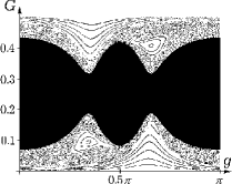
Figure 6: $H=0.5,\;E=-3.3$

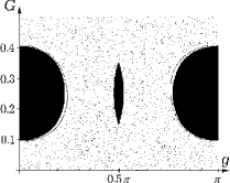
Figure 8: $H=0.5,\;E=-3.6$

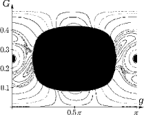
Figure 10: $H=0.5,\;E=-7.5$

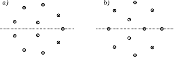
Figure 11:

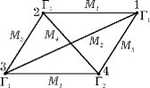
Figure 12:

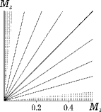
a) $\begin{aligned} \Gamma_{1}&=-1.5,\\ \Gamma_{2}&=2.0.\end{aligned}$	b) $\begin{aligned} \Gamma_{1}&=-0.183,\\ \Gamma_{2}&=2.0.\end{aligned}$	c) $\begin{aligned} \Gamma_{1}&=-0.183,\\ \Gamma_{2}&=0.683.\end{aligned}$

Figure 13:

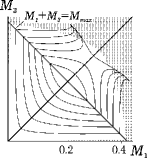
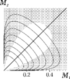
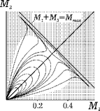
a) $\begin{aligned} \Gamma_{1}&=-0.183,\\ \Gamma_{2}&=2.0,\\ k&=0.6.\end{aligned}$	b) $\begin{aligned} \Gamma_{1}&=-1.5,\\ \Gamma_{2}&=2.0,\\ k&=0.6.\end{aligned}$	c) $\begin{aligned} \Gamma_{1}&=-0.183,\\ \Gamma_{2}&=0.683,\\ k&=0.6.\end{aligned}$

Figure 14:

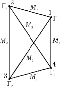
Figure 15:

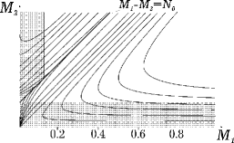
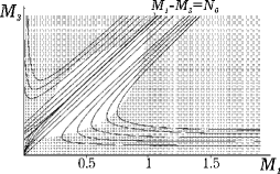
$\begin{aligned} \Gamma_{1}&=2.0,\;&\Gamma_{2}&=2.0\\ k&=0.0,\;&D&=-2.0.\end{aligned}$	$\begin{aligned} \Gamma_{1}&=2.0,\;&\Gamma_{2}&=2.0\\ k&=0.9,\;&D&=-2.0.\end{aligned}$
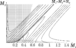
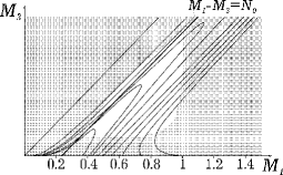
$\begin{aligned} \Gamma_{1}&=-1.0,\;&\Gamma_{2}&=2.0\\ k&=0.0,\;&D&=-2.0.\end{aligned}$	$\begin{aligned} \Gamma_{1}&=-1.0,\;&\Gamma_{2}&=2.0\\ k&=0.9,\;&D&=-2.0.\end{aligned}$
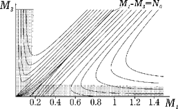
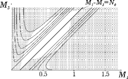
$\begin{aligned} \Gamma_{1}&=-1.8,\;&\Gamma_{2}&=2.0\\ k&=0.0,\;&D&=-2.0.\end{aligned}$	$\begin{aligned} \Gamma_{1}&=-1.8,\;&\Gamma_{2}&=2.0\\ k&=0.9,\;&D&=-2.0.\end{aligned}$
a)	b)

Figure 16:

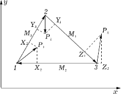
Figure 17:

References

- [1] H. Aref. On the equilibrium and stability of a row of point vortices. J. Fluid Mech., v. 290, 1995, p. 167–191.
- [2] H. Aref. Integrable, chaotic and turbulent vortex motion in two-dimensional flows. Ann. Rev. Fluid Mech., v. 15, 1983, p. 345–389.
- [3] H. Aref. Point vortex motions with a center of symmetry. Phys. Fluids, 1982, v. 25 (12), p. 2183–2187.
- [4] H. Aref, D. L. Vainstein. Point vertices exhibit asymmetric equilibria. Nature, v. 392, 1998, 23 April, p. 769–770.
- [5] V. I. Arnold, V. V. Kozlov, A. I. Neishtadt. Mathematical aspects of classical and celestial mechanics. 2nd ed. Encyclopedia of Mathematical Sciences, v. 3 (Dynamical systems III), New York, Springer, 1996.
- [6] V. I. Arnold. Mathematical methods of classical mechanics. New York, Springer, v. 60., 1984.
- [7] V. I. Arnold, A. B. Givental. Symplectic geometry. M., VINITI, v. 4, 1985, p. 5–140.
- [8] A. Barut, R. Raczka. Theory of Group Representations and Applications. PWN. Polish Scientific Publishers, 1977.
- [9] V. A. Bogomolov. Dynamics of the vortisity on a sphere. Izv. AN USSR, Mekh. zhid. gaza, No. 6, 1977, p. 57–65.
- [10] A. V. Bolsinov. Compatible Poisson brackets on Lie algebras and the completeness of families of involutive functions Izv. AN USSR, ser. math., v. 55, 1991, No. 1, p. 68–92.
- [11] A. V. Bolsinov, A. V. Borisov. Lax-representation and compatible Poisson brackets on Lie algebras. (to be published, 1999).
- [12] A. V. Borisov, K. V. Emelyanov. Non-integrability and stochastisity in rigid-body dynamics. Izhevsk, Izd. Udm. Univ., 1995.
- [13] A. V. Borisov, A. E. Pavlov. Dynamics and Statics of Vortices on a Plane and a Sphere — I. Reg. & Ch. Dynamics, v. 3, 1998, No. 1, p. 28–39.
- [14] A. V. Borisov, V. G. Lebedev. Dynamics of Three Vortices on a Plane and a Sphere — II. General compact case. Reg. & Ch. Dynamics, v. 3, 1998, No. 2, p. 99–114.
- [15] A. V. Borisov, V. G. Lebedev. Dynamics of three vortices on a plane and a sphere — III. Noncompact case. Problem of collapse and scattering. Reg. & Ch. Dynamics, v. 3, 1998, No. 4, p. 76–90.
- [16] L. J. Campbell, R. M. Ziff. Vortex patterns and energies in a rotation superfluid. Phys. Rev. B., v. 20, 1979, No. 5, p. 1886–1901.
- [17] D. N. Goryachev. On some cases of the motion of straightline vortices. Moskwa, 1898.
- [18] A. T. Fomenko. Symplectic geometry. .: GU, 1988.
- [19] C. G. J. Jacobi. Vorlesungen über Dynamik. Aufl. 2. Berlin: G. Reimer, 1884, 300 S.
- [20] E. R. van Kampen, A. Wintner. On a symmetrical canonical reduction of the problem of three bodies. Amer. J. Math., v. 59, 1937, No. 1, p. 153–166.
- [21] G. Kirchhoff. Vorlesungen über mathematische Physik. Leipzig, 1891, 272 S.
- [22] J. Marsden, A. Weinstein. Reduction of Symplectic manifolds with symmetry. Rep. on Math. Phys., v. 5, 1974, No. 5, p. 121–130.
- [23] V. V. Meleshko, M. Yu. Konstantinov. Dynamics of vortex structures. Kiev, Naukova Dumka, 1993.
- [24] E. A. Novikov, Yu. B. Sedov. Collapse of vortices. ZETF, v. 77, No. 2(8), 1979, p. 588–597.
- [25] C. L. Charlier. Die Mechanik des Himmels. Walter de Gruyter & Co. 1927.
- [26] S. Smeil. Topology and mechanics. Uspekhi mat. nauk, v. 27, No. 2, 1972, p. 77–133.
- [27] E. T. Whittaker. A treatise on the analytical dynamics. Ed. 3-d. Cambridge Univ. Press., 1927.
- [28] A. Wintner. The analytical foundation of celestial mechanics. Princeton Univ. Press, 1941.