Coupled mode theory for photonic band-gap inhibition of spatial instabilities

Abstract

We study the inhibition of pattern formation in nonlinear optical systems using intracavity photonic crystals. We consider mean field models for single and doubly degenerate optical parametric oscillators. Analytical expressions for the new (higher) modulational thresholds and the size of the ”band-gap“ as function of the system and photonic crystal parameters are obtained via a coupled-mode theory. Then, by means of a nonlinear analysis, we derive amplitude equations for the unstable modes and find the stationary solutions above threshold. The form of the unstable mode is different in the lower and upper part of the bandgap. In each part there is bistability between two spatially shifted patterns. In large systems stable wall defects between the two solutions are formed and we provide analytical expressions for their shape. The analytical results are favorably compared with results obtained from the full system equations. Inhibition of pattern formation can be used to spatially control signal generation in the transverse plane.

I Introduction

Photonic crystals (PC) have shown to be able to control light in ways that were not possible with conventional optics Joannopoulos ; Knight . Their remarkable properties stem from the unusual dispersion relation as a result of the periodic modulation of their dielectric properties. Most of the interest on PC is related to propagation problems. Here the existence of photonic band-gaps, i.e. a range of frequencies for which light can not propagate in the medium, allows for a new way of guiding and localize light once defects are introduced in the PC Joannopoulos ; Knight . Photonic crystals in combination with nonlinear effects have been also considered for all-optical switching devices Slusher .

Transverse effects in periodic media have been mainly studied in propagation in planar waveguides with periodic modulation of the refractive index in the transverse direction and arrays of couple waveguides. In the first case the attention has been focused on the so called spatial gap (or Bragg) solitons Kivshar ; Nabiev ; Yulin , which are intense peaks with frequencies inside the (linear) band-gap. This is possible thanks to a shift of the photonic band-gap boundaries due to nonlinear effects: the intense core of a gap soliton can propagate freely in the periodic media, while in its less intense tails, where non-linearity can be neglected, light is reflected back to the center due to Bragg reflection, sustaining the localized structure. Bragg solitons are usually studied within the coupled-mode theory where only the slowly varying envelope of two counter-propagating beams are considered. Arrays of waveguides are usually studied within the tight-binding approximation, where the system is described by a set of coupled ordinary differential equations describing the dynamics of the guided-mode amplitude in each site. The evanescent coupling between adjacent waveguide give rise to the so called discrete diffraction. If nonlinearity is also present discrete solitons can be formed Slusher ; Kivshar .

In this paper we consider a different case, a photonic crystal inside a nonlinear optical cavity, i.e. a system with driving and dissipation. Nonlinear optical cavities typically undergo spatial instabilities leading to the formation of spatial structures similar to what observed in many different fields across science Cross-Hohenberg ; Walgraef . In particular, spatial structures in nonlinear optical cavities have important potential applications in photonics such as memories, multiplexing, optical processing and imaging Firth . Control of spatial structures is then an important issue for the implementation of such devices. In this context, different mechanisms of control have been proposed Martin ; Harkness ; Neubecker . In particular, Neubecker and Zimmerman reported on experimental pattern formation in presence of an external modulated forcing and observed lockings between the forcing and natural wavelengths Neubecker . More recently the use of the properties of photonic crystals for the control of optical spatial structures has been considered PRL ; Dabbicco ; Choquette . In PRL we showed how the photonic band-gap of a photonic crystal could be used to inhibit a pattern forming instability in a self-focusing Kerr cavity. Pattern formation in an optically-injected, photonic-crystal vertical-cavity surface-emitting laser, electrically biased below threshold has been observed experimentally in Dabbicco . Finally, in Choquette , a defect in a photonic crystal has been used to achieve stable emission in broad area lasers.

Here we study the inhibition of pattern formation in a mean field model for a Degenerate Optical Parametric Oscillator with a photonic crystal. We first show that the inhibition mechanism introduced in PRL occurs independently of the type of nonlinearity here being quadratic. Then we introduce an analytical treatment by means of a couple-mode theory that fully explains the phenomenon. A linear stability analysis allows us to determine analytically the new thresholds shifted in parameter space by pattern inhibition and the form of the unstable modes. We show that the band-gap region is divided into two different regions: one in which pattern formation takes place due to an energy concentration at the maxima of the photonic crystal modulation, and a different one where the energy concentrates at the minima. We determine amplitude equations for the unstable modes and find the stationary solutions above threshold analytically. We show that this scenario is organized by a co-dimension two bifurcation point where both modes become simultaneously unstable. We also show that in the band-gap, where the pattern arises with a wavenumber half the one of the PC, there is bistability between two different ”phase locked” solutions differing by a shift of a PC wavelength in the near field. This bistability stems from the breaking of the translational symmetry by the PC. In large systems this leads to the formation of domains of different ”phases” connected by topological walls (or antiphase boundaries) Walgraef . This is a different kind of (spatial) bistability where the two different ”phases” do not differ on the phase of the electric field but on the location of the spatial oscillation in the near field.

II Models

A phase-matched Double Resonant Degenerate Optical Parametric Oscillator (DRDOPO), where both pump and signal fields resonate in the cavity, can be described in the mean field approximation by refsDRDOPO :

$$\partial_{t}B = \Gamma[-B+E-A^{2}]+i{1\over 2}\partial_{xx}B$$

$$\partial_{t}A = -A-i\Delta_{s}A+BA^{*}+i\partial_{xx}A,$$ (1)

where $B$ and $A$ are the pump and signal slowly varying amplitudes, $\Gamma$ is the ratio between the pump and signal cavity decay rates and $E$ is the amplitude of the external pump field (our control parameter). $\Delta_{s}=\Delta+\alpha f(x)$ is the total signal detuning, where $\Delta$ is the average detuning and $f(x)=e^{ik_{pc}x}+e^{-ik_{pc}x}$ describes the spatially dependent contribution of the photonic crystal (Fig. 1).

For the singly resonant DOPO (SRDOPO), where there is no cavity for the pump field, the mean field equation for the resonating signal is refsSRDOPO ; G-L

$$\partial_{t}A=-A-i\Delta_{s}A+EA^{*}-|A|^{2}A+i\partial_{xx}A.$$ (2)

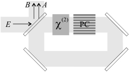
Figure 1: Scheme of a doubly resonant degenerate optical parametric oscillator with a photonic crystal. It consist of a ring cavity filled with a quadratic ($\chi^{(2)}$) medium and a photonic crystal slab (PC). $E$ is the plane wave input field at frequency $\omega$ partially transmitted into the cavity. The other mirrors are assumed to be perfectly reflecting. $B$ and $A$ are the pump and signal fields at frequencies $\omega$ and $\omega/2$ respectively. In the single resonant case only the signal field $A$ resonates with the cavity.

III Linear stability analysis with periodic media: couple-mode theory

The linearization around the steady state homogeneous solution $B^{0}=E$ and $A^{0}=0$ of Eqs. (II) and (2) leads, in both cases, to the same equation for the perturbations of the signal $A$:

$$\partial_{t}A=-(1+i\Delta)A-i\alpha f(x)A+EA^{*}+\partial_{xx}A.$$ (3)

Without the photonic crystal ($\alpha=0$), the homogeneous solution is stable for $E<1$. Above threshold ($E>1$) a stripe pattern arises with a wavenumber $k_{c}=\sqrt{-\Delta}$. Here we restrict ourselves to negative values of the detuning. For positive detuning the system display bistability between homogeneous solutions G-L . For $\alpha\neq 0$, and assuming that the amplitude of the modulation is weak enough, we can write the signal perturbations as a superposition of two waves with opposite transverse wavenumbers Yulin

$$A=A_{+}(x,t)e^{ik_{pc}x/2}+A_{-}(x,t)e^{-ik_{pc}x/2},$$ (4)

where $A_{\pm}(x,y)$ are slow functions of $x$. This is basically equivalent to the so called coupled-mode theory for propagation of pulses in periodic media Slusher .

By writing $A_{\pm}=a_{\pm}^{+}(t)e^{ikx}+a_{\pm}^{-}(t)e^{-ikx}$, one obtains a set of coupled linear ordinary differential equations for the amplitudes $a_{\pm}^{+}$ ($a_{\pm}^{-}$) of the Fourier components $\pm k_{pc}/2+k$ ($\pm k_{pc}/2-k$) of the perturbations. By defining ${\bf F}=(a_{+}^{+},a_{-}^{-*},a_{-}^{+},a_{+}^{-*})^{T}$ this set of equations can be written as

$$\dot{\bf F}={\mathcal{L}}{\bf F},$$ (5)

where ${\mathcal{L}}$ is given by

$${\mathcal{L}}=\left(\begin{array}[]{cccc}-1-i\Delta-i(k+{k_{pc}\over 2})^{2}&E&-i\alpha&0\\ E&-1+i\Delta+i(k+{k_{pc}\over 2})^{2}&0&i\alpha\\ -i\alpha&0&-1-i\Delta-i(k-{k_{pc}\over 2})^{2}&E\\ 0&i\alpha&E&-1+i\Delta+i(k-{k_{pc}\over 2})^{2}\end{array}\right).$$ (6)

In this way one reduces the stability analysis of the steady state of the initial partial differential equations with periodic coefficients (II) and (2) to diagonalize the $4\times 4$ complex matrix ${\mathcal{L}}$. In the case $k=0$ one has to consider that $a_{\pm}^{+}=a_{\pm}^{-}$.

The eigenvalue of ${\mathcal{L}}$ with largest real part is

$$\lambda=-1+\sqrt{E^{2}-\left[k^{2}+\left({k_{pc}\over 2}\right)^{2}+\Delta-\sqrt{\alpha^{2}+4k^{2}\left({k_{pc}\over 2}\right)^{2}}\right]^{2}},$$ (7)

and by setting $\lambda=0$ we obtain four marginal stability curves

$$\Delta_{1}(k,E) = -d_{1}(k)+d_{2}(k)+d_{3}(E)$$

$$\Delta_{2}(k,E) = -d_{1}(k)+d_{2}(k)-d_{3}(E)$$

$$\Delta_{3}(k,E) = -d_{1}(k)-d_{2}(k)+d_{3}(E)$$

$$\Delta_{4}(k,E) = -d_{1}(k)-d_{2}(k)-d_{3}(E).$$ (8)

where $d_{1}(k)=\left(k_{pc}/2\right)^{2}+k^{2}$, $d_{2}(k)=\sqrt{4k^{2}\left({k_{pc}/2}\right)^{2}+\alpha^{2}}$ and $d_{3}(E)=\sqrt{E^{2}-1}$.

Fig. 2 shows the marginal stability curves for different values of the pump $E$. Note that, due to definition (4), $k=0$ indicates a perturbation with a wavenumber at the limit of the first Brillouin zone. Therefore it is convenient to plot $\Delta$ as a function of $k^{\prime}=(k_{pc}/2-k)/k_{pc}$. Dotted lines are the results from the coupled-mode theory (III), while solid lines have been obtained from a numerical stability analysis of the full model, i.e. solving the eigenvalue problem associated to the linear differential operator with periodic coefficients in the rhs of (3) PRL . The coupled-mode theory provides a very good analytical approximation for thresholds and unstable wavenumbers allowing us to predict the existence and size of a band-gap in the modulation instability analytically. In the following we analyze the results of the coupled-mode theory in more detail.

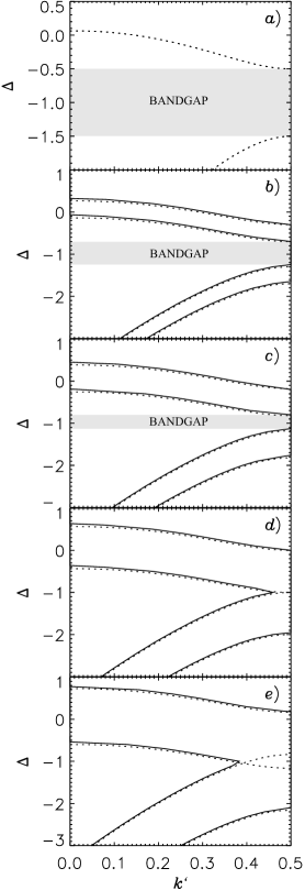
Figure 2: Unstable wavenumbers of a DOPO for $a)E=1.0$, $b)E=1.02$, $c)E=1.05$, $d)E=\sqrt{1+\alpha^{2}}=1.118034$, and $e)E=1.2$ in presence of a periodically modulated media ($k_{pc}=2,\alpha=0.5$). For each value of $\Delta$ wavenumbers between the two lines are unstable.

From (III) one can evaluate the instability threshold of the fundamental solution as a function of the detuning $\Delta$. For $E<1.0$ the steady state homogeneous solution is stable for all values of the detuning. At $E=1$ (Fig. 2a) $d_{3}(E)=0$ and the four marginal stability lines given by Eqs. (III) become only two, signaling the instability threshold for all values of the detuning outside the band-gap ($-d_{1}(k_{pc}/2)-d_{2}(k_{pc}/2)+\alpha^{2}<\Delta<-(k_{pc}/2)^{2}-\alpha<-(k_{pc}/2)^{2}+\alpha<\Delta<-d_{1}(k_{pc}/2)+d_{2}(k_{pc}/2)+\alpha^{2}$). In the bandgap, $-(k_{pc}/2)^{2}-\alpha<\Delta<-(k_{pc}/2)^{2}+\alpha$, the instability is, however, inhibited. The threshold $E=1$ for values of $\Delta$ outside the bandgap is slightly underestimated. In the full model, for this value of the pump, the system is still stable (no solid line in Fig.2a). This is due to the fact that the spatial modulation couples the fundamental wavenumbers with their harmonics, which are dumped, introducing an additional source of stability. Harmonics are not taken into account in the couple-mode theory and then the threshold is slightly lower than for the full models (II) and (2).

Increasing further the value of the pump the band-gap narrows (Figs 2b,c). At $E=\sqrt{1+\alpha^{2}}$ the homogeneous solution become eventually unstable for any value of the detuning (Fig. 2d). The threshold value of $E$ as a function of the photonic crystal parameters for any value of $\Delta$ is given by

$$E^{2}_{th}(\Delta)=\left\{\begin{array}[]{ccccc}1&&-({k_{pc}\over 2})^{2}+\alpha&<\Delta\leq&-d_{1}({k_{pc}\over 2})+d_{2}({k_{pc}\over 2})+\alpha^{2}\\ 1+\left[-({k_{pc}\over 2})^{2}+\alpha-\Delta\right]^{2}&&-({k_{pc}\over 2})^{2}&<\Delta\leq&-({k_{pc}\over 2})^{2}+\alpha\\ 1+\left[({k_{pc}\over 2})^{2}+\alpha+\Delta\right]^{2}&&-({k_{pc}\over 2})^{2}-\alpha&<\Delta\leq&-({k_{pc}\over 2})^{2}\\ 1&&-d_{1}({k_{pc}\over 2})-d_{2}({k_{pc}\over 2})+\alpha^{2}&<\Delta\leq&-({k_{pc}\over 2})^{2}-\alpha\end{array}\right.,$$ (9)

and the critical wavenumber by:

$$k^{2}_{c}(\Delta)=\left\{\begin{array}[]{ccccc}(k_{pc}/2)^{2}-\Delta-\sqrt{-4({k_{pc}\over 2})^{2}\Delta+\alpha^{2}}&&-({k_{pc}\over 2})^{2}+\alpha&<\Delta\leq&-d_{1}({k_{pc}\over 2})+d_{2}({k_{pc}\over 2})+\alpha^{2}\\ 0&&-({k_{pc}\over 2})^{2}&<\Delta\leq&-({k_{pc}\over 2})^{2}+\alpha\\ 0&&-({k_{pc}\over 2})^{2}-\alpha&<\Delta\leq&-({k_{pc}\over 2})^{2}\\ ({k_{pc}\over 2})^{2}-\Delta-\sqrt{-4({k_{pc}\over 2})^{2}\Delta+\alpha^{2}}&&-d_{1}({k_{pc}\over 2})^{2}-d_{2}({k_{pc}\over 2})+\alpha^{2}&<\Delta\leq&-({k_{pc}\over 2})^{2}-\alpha\end{array}\right..$$ (10)

Fig. 3 shows the theoretical prediction (9) for the instability threshold of the homogeneous solution (solid lines). The black and grey lines correspond to two different eigenmodes. The first is a mode with energy concentrated in the minima of the photonic crystal, while the second in the maxima (see next section for more details). The dashed line is the threshold for the full system computed as explained above.

The coupled-mode theory accurately capture the features of the inhibition of the modulation instability by the photonic crystal. The fact that the gap of values of the detuning for which pattern formation is inhibited decreases with the intensity of the pump is because nonlinearity always overcomes the linear inhibition by the photonic crystal for suitable high input intensities. This is similar to the phenomenon behind the formation of gap solitons. But in that case the nonlinearity only shifts the position of the band-gap, while in our case it narrows it and makes it eventually to disappear.

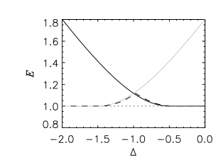
Figure 3: Pump threshold as function of the detuning from the theoretical result (9) obtained by means of the coupled-mode theory (solid black and grey lines). The dashed line is the result obtained from a numerical stability analysis of the full model. The dotted line is the threshold for a DOPO without photonic crystal.

From Eq. (9) we can calculate the size $g(E,\alpha)$ of the band-gap as function of the system and photonic crystal parameters:

$$g(E,\alpha)=2(\alpha-\sqrt{E^{2}-1}).$$ (11)

The size of the band-gap is proportional to the amplitude of the modulation $\alpha$ and becomes smaller by increasing the pump $E$ (Fig. 2), eventually disappearing for $E=\sqrt{1+\alpha^{2}}$ (Fig. 2d). For $E>1+\alpha^{2}$ the homogeneous solution is unstable for any value of $\Delta$ (Fig. 2e). Fig. 4 shows how the width of the band-gap (white region) changes as function of the amplitude of the modulation $\alpha$ for a fixed value of the pump $E$. The presence of the modulated medium opens an entirely new stable region. Fig. 4 should be compared with Fig. 6 of PRL showing that pattern inhibition is independent of the form of the nonlinearity.

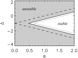
Figure 4: Stability diagram of the steady state homogeneous solution for $E=1.1$ (solid line). The system is unstable in the shadowed region. The dashed (dotted) line shows the boundary of the stable region for $E=1.0$ ($E=1.2$).

Since for negative signal detunings, in the absence of PC, down conversion takes place at a finite wavenumber, the inhibition mechanism can be used to spatially control the generation of signal in a way analogous to that explained in PRL . If we set our system in a parameter region where pattern formation is inhibited, the inclusion of a defect in the PC will lead to a spot of signal generation as shown in Fig. 5.

Figure 5: Localized spot of signal generation due to a defect in the photonic crystal. Here $E=1.08,\Delta=-1,k_{pc}=2$ and $\alpha=0.5$.

IV Weakly nonlinear analysis: amplitude equations for pattern formation in periodic media

In this section we study by means of a multiple scales analysis the solutions that appear above threshold for values of the detuning inside the band-gap. Above threshold nonlinear terms have to be considered since they saturate the linear growth induced by the instability. In the following we consider the SRDOPO only. By including the nonlinear terms from (2) in (5) we obtain:

$$\dot{\bf F}={\mathcal{L}}{\bf F}-{\mathcal{W}}({\bf F}),$$ (12)

where ${\mathcal{W}}=[(a_{+}^{+}a_{+}^{-*}+2a_{-}^{-*}a_{-}^{+})a_{+}^{+},(2a_{-}^{+}a_{-}^{-*}+a_{+}^{-*}a_{+}^{+})a_{-}^{-*}(a_{-}^{+}a_{-}^{-*}+2a_{+}^{-*}a_{+}^{+})a_{-}^{+},(2a_{+}^{+}a_{+}^{-*}+a_{-}^{-*}a_{-}^{+})a_{+}^{-*}]^{T}$ is a nonlinear function of ${\bf F}$.

In the bandgap, the critical wave number is always $k_{c}=0$ independently of the detuning. We recall that in this case one has to consider $a_{\mp}^{+}=a_{\mp}^{-}$. In the following we will discuss the lower ($-(k_{pc}/2)^{2}-\alpha\leq\Delta<-(k_{pc}/2)^{2}$) and upper ($-(k_{pc}/2)^{2}\leq\Delta<-(k_{pc}/2)^{2}+\alpha$) halves of the band-gap separately.

IV.1 Lower-half part

Assuming the following scaling refsDRDOPO :

$${\bf F} = \epsilon{\bf F_{1}}+\epsilon^{3}{\bf F_{3}}$$ (13)

$$E = E_{th}+\epsilon^{2}E_{2}$$

$$T = \epsilon^{2}t$$

$$X = \epsilon^{2}x.$$

Substituting (13) in (12), at order $\epsilon$ one obtains ${\bf F_{1}}=F_{1}{\bf v_{1}}$, where ${\bf v_{1}}$ is the critical eigenmode of ${\mathcal{L}}$ (${\mathcal{L}}{\bf v_{1}}=0$ and $|{\bf v_{1}}|=1$) and $F_{1}$ is its real amplitude. In the near field, ${\bf v_{1}}$ has the form: $[(1+E_{th}-i\sqrt{E_{th}^{2}-1})/\sqrt{2E_{th}(1+E_{th})}]\cos(k_{pc}x/2)$.

The solvability condition at order $\epsilon^{3}$ yields to the following equation for the real amplitude $\tilde{A_{1}}=\epsilon F_{1}$ of the unstable mode

$$\partial_{t}\tilde{A_{1}}=\sqrt{E_{th}^{2}-1}~{}\partial_{x}^{2}\tilde{A_{1}}+E_{th}(E-E_{th})\tilde{A_{1}}-{3\over 4}\tilde{A_{1}}^{3}.$$ (14)

The amplitude equation (14) is equivalent to the one obtained from a secondary instability at twice the spatial period of a cellular pattern Coullet , except for the fact that in our case the translational invariance has been broken by the presence of the photonic crystal. The homogeneous steady state solution of (14) is $\tilde{A_{1}}=\pm 2\sqrt{E_{th}(E-E_{th})/3}$. The solution of (2) is then:

$$A(x)=\pm\sqrt{2\over 3}\sqrt{E-E_{th}\over 1+E_{th}}\left(1+E_{th}-i\sqrt{E_{th}^{2}-1}\right)\cos({k_{pc}\over 2}x).$$ (15)

The bifurcation diagram and spatial form of this solution is shown in Fig 6. The plus and minus solutions (15) are created in a pitchfork bifurcation. The analytical solution (15) is in very good agreement with the stationary solution of the full model computed numerically. Note that, despite being completely equivalent, the plus and minus solutions of (15) are not the same. One corresponds to the other shifted by a wavelength of the photonic crystal modulation. In a system with translational invariance the position of a solution that brakes such symmetry is undetermined. The photonic crystal periodicity selects just two of a continuum of possible solutions. This two ”frequency locked” solutions differ now by a shift of a photonic crystal wavelength in the transverse position. This situation is the spatial analogue of an oscillatory system forced at twice its natural frequency Coullet2 . In a large system and starting from arbitrary initial conditions, some sections of the system will attain the first solution while others will move to the second one, leading to the formation of domain walls. This is illustrated in Fig. 7. The solid line is the result of a simulation of the full model (2) starting from a random initial condition. The dashed line is the steady state solution of Eq. (14) connecting the two (plus and minus) homogeneous solutions Walgraef times the critical eigenmode ${\bf v_{1}}$ in the near field:

$$A_{1}(x)=\sqrt{2\over 3}\sqrt{E-E_{th}\over 1+E_{th}}\left(1+E_{th}-i\sqrt{E_{th}^{2}-1}\right)\tanh\left[\sqrt{E_{th}(E-E_{th})\over 2}{x\over(E_{th}^{2}-1)^{1\over 4}}\right]\cos({k_{pc}\over 2}x).$$ (16)

The dotted-dashed line in Fig. 7 is the envelope of (16). The analytical result (16) is in very good agreement with the domain wall obtained from the numerical simulations of the full model (2).

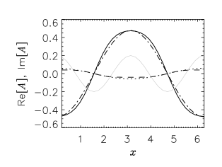
Figure 6: Left: Bifurcation diagram for the pattern arising above threshold in the lower-half of the band-gap. Here $\Delta=-1.2$. For this value of the detuning $E_{th}=1.04403$. Right: Real (solid line) and imaginary (dashed lined) of the pattern solution of the full model for $E=1.2$. The dot-dashed and dotted lines correspond to the real and imaginary parts of the pattern from the coupled-mode theory. The grey solid line illustrates the modulation of the photonic-crystal for comparison.

Figure 7: Two domains corresponding to the plus and minus sign solutions (15) separated by domain walls. The final state is the result of a numerical simulation starting from an arbitrary initial condition. Left: Real part of the field. Right: Close up to the intensity around a domain wall. The dotted line shows the modulation of the photonic crystal. Here $\Delta=-1.1$, $E=1.15$, $\alpha=0.5$ and $k_{pc}=2.0$.

IV.2 Upper-half part

In the upper-half part of the photonic band-gap the critical mode ${\bf v_{1}}$ has the form: $\{[\sqrt{E_{th}^{2}-1}+i(E_{th}-1)]/\sqrt{2E_{th}(E_{th}-1)}\}\sin(k_{pc}x/2)$. As in the previous case, we obtain a similar amplitude equation for the real amplitude $\tilde{A_{1}}$ of the unstable mode

$$\partial_{t}\tilde{A_{1}}=\sqrt{E_{th}^{2}-1}~{}\partial_{x}^{2}\tilde{A_{1}}+\sqrt{E-E_{th}}\tilde{A_{1}}-{3\over 4}\tilde{A_{1}}^{3}.$$ (17)

In this case the pattern solutions is

$$A_{1}(x)=\pm\sqrt{2\over 3}\sqrt{E-E_{th}\over E_{th}(E_{th}-1)}\left[\sqrt{E_{th}^{2}-1}+i(E_{th}-1)\right]\sin({k_{pc}\over 2}x).$$ (18)

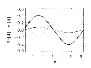
Figure 8: Left: Bifurcation diagram for the pattern arising above threshold in the lower-half of the band-gap. Here $\Delta=-0.9$. For this value of the detuning $E_{th}=1.07703$. Right: Real (solid line) and imaginary (dashed lined) of the pattern solution of the full model for $E=1.2$. The dot-dashed and dotted lines correspond to the real and imaginary parts of the pattern from the coupled-mode theory. The grey solid line illustrates the modulation of the photonic-crystal for comparison.

The bifurcation diagram and spatial form of this solution is shown in Fig 8. The analytical solution (18) is in very good agreement with the stationary solution of the full model computed numerically. As in the previous case, in large systems, fronts between the plus and minus solutions are formed. The shape of the front is given by:

$$A_{1}(x)=2\sqrt{2\over 3}\sqrt{E-E_{th}\over E_{th}(E_{th}-1)}\left[\sqrt{E_{th}^{2}-1}+i(E_{th}-1)\right]\tanh\left[\sqrt{E-E_{th}\over 2}{x\over(E_{th}^{2}-1)^{1\over 4}}\right]\sin({k_{pc}\over 2}x).$$ (19)

Note that while the cosine solution in the lower-half part of the band-gap has the maxima of the intensity at the maxima of the photonic crystal modulation, the sine solution in the upper-part has them at the minima. This different distribution of energy in the photonic crystal is at the basis of the creation of the band-gap. An interesting point is the middle of the band-gap ($\Delta=-(k_{pc}/2)^{2}$). At this particular value of the detuning, for $E=E_{th}=\sqrt{1+\alpha^{2}}$ both the sine and cosine modes become simultaneously unstable. This is a co-dimension two point where Eqs. (14) and (17) become coupled. The unfolding of such a critical point is however beyond the scope of this paper and it is left for future investigation.

V Conclusions

In this paper we have studied pattern formation in nonlinear optical cavities in presence of a photonic crystal, i.e. a spatial modulation of the refractive index. The linear phenomenon of the band-gap inhibits pattern formation for a certain range of cavity detunings (bandgap). For high enough intensities nonlinearity finally overcomes the inhibition by the photonic crystal and a pattern arises. By means of a couple-mode theory approach we have obtained analytical expressions for the new (shifted) threshold and the form of the unstable modes. The bandgap is naturally divided in two halves, the lower-half one in which the unstable mode has a cosine shape, i.e. its intensity maximums are in correspondence with the maximums of the photonic crystal modulation, and the upper-half where the unstable mode is a sine; the intensity maximums are in correspondence with the minima of the photonic crystal modulation. By means of a multiple scale analysis we also found the pattern solution above threshold. In each part of the bandgap there is bistability between the plus and minus cosine or sine solutions. This bistability stems from the breaking of the translational symmetry of the photonic crystal. In large systems domain wall between this two solutions are typically form. The shape of the defect wall is given by an hyperbolic tangent. While the particular form of the coefficients are model dependent, the shape of the unstable modes and the splitting of the bandgap in two different regions are generic. We have checked that the same phenomenon is present in a completely different model, namely the Kerr cavity model studied in PRL . Finally we also have shown that photonic crystal can be useful to engineer particular spatial signal outputs in frequency down conversion. An interesting extension of this work is to consider the case with two transverse dimension. In this case, some of the features studied here, such us the two different modes in each part of the bandgap, will remain the same, while new features like the coupling of the geometry of the photonic crystal and that of the spontaneous pattern will come into play.

- (1) J.D. Joannopoulos, R.D. Meade, and J.N. Winn, Photonic Crystals (Princeton University Press, Singapore, 1995); J.D. Joannopoulos, P.R. Villeneuve, and S. Fran, Nature (London) 386, 143 (1997).
- (2) J.C. Knight, Nature (London) 424, 846 (2003).
- (3) Nonlinear Photonic Crystals, edited by R.E. Slusher and B.J. Eggleton (Springer, Berlin, 2003).
- (4) Y.S. Kivshar and G.P. Agrawal, Optical Solitons: From Fibers to Photonic Crystals (Academic Press, San Diego, 2003); Spatial Solitons, edited by S. Trillo and W. Torruellas (Springer, Berlin, 2001).
- (5) R.F. Nabiev, P. Yeh, and D. Botez, Optics Lett. 18, 1612 (1993).
- (6) A.V. Yulin, D.V. Skryabin and W.J. Firth, Phys. Rev. E 66, 046603 (2002).
- (7) M.C. Cross and P.C. Hohenberg, Rev. Mod. Phys. 65, 851 (1993)
- (8) D. Walgraef, Spatio-temporal pattern formation (Springer-Verlag, New York, 1997).
- (9) W.J. Firth and C.O. Weiss, Opt. Phot. News 13, 55 (2002); S. Barland et al., Nature 419, 699 (2002).
- (10) R. Martin et al., Phys. Rev. Lett. 77, 4007 (1996).
- (11) G. Harkness et al., Opt. Phot. News, December 1998, 44.
- (12) R. Neubecker and A. Zimmermann, Phys. Rev. E 65, 035205(R) (2002).
- (13) D. Gomila, R. Zambrini and G.-L. Oppo, Phys. Rev. Lett. 92, 253901 (2004).
- (14) M. Dabbicco, T. Maggiopinto and M. Brambilla, Appl. Phys. Lett., to appear (2004).
- (15) T.S. Kim el al., Electr. Lett. 40, 1340 (2004).
- (16) G.-L. Oppo, M. Brambilla and L.A. Lugiato, Phys. Rev. A 49, 2028 (1994); G.-L. Oppo et al., J. Mod. Opt. 41, 1151 (1994).
- (17) S. Longhi, J. Mod. Opt. 43, 1089 (1996).
- (18) G.-L. Oppo, A.J. Scroggie, and W.J. Firth, Phys. Rev. E 63, 066209 (2001).
- (19) P. Coullet and G. Iooss, Phys. Rev. Lett. 64, 866 (1990).
- (20) P. Coullet et all., Phys. Rev. Lett. 65, 1352 (1990). P. Coullet and K. Emilsson, Physics (Amsterdam) 61D, 119 (1992).