Convective instability induced by nonlocality in nonlinear diffusive systems

Abstract

We consider a large class of nonlinear diffusive systems with nonlocal coupling. By using a non-perturbative analytical approach we are able to determine the convective and absolute instabilities of all the uniform states of these systems. We find a huge window of convective instability that should provide a great opportunity to study experimentally and theoretically noise sustained patterns.

There has been a considerable interest in convective instabilities and noise induced patterns recently santagiustina97-taki00 . A convective instability happens when a state of a nonlinear system becomes unstable and a localised perturbation grows travelling in the system, but eventually decays at any point in the laboratory frame. In this regime a state different from the original one cannot be established unless it is sustained by noise. Small regions of convective instabilities have been predicted and observed in hydrodynamics ahlers83-gondret99 , plasma physics briggs and optics Louvergeaux04 . These are due to spatial drift terms modelled by gradients in the direct space or by the first few terms of the Taylor expansion of the dispersion relation in the Fourier space Louvergeaux04 .

In this letter, instead, we study nonlinear systems with nonlocal coupling. Nonlocality is fundamental in modelling material response in presence of transport effects nonlocalrefs . Even for local material response, nonlocality is unavoidable whenever travelling waves emerging from a medium are reflected back to it non-collinearly, therefore coupling any spatial point $x$ with the shifted point $x+\Delta x$. Indeed this kind of nonlocal coupling is induced by any small misalignment in all feedback optical systems (see experiments in Refs. ramazza98 ; Louvergeaux04 ; thorsten99 ). We consider the most general case in which the spatial shift cannot be approximated by a gradient (drift) term in a very broad class of nonlinear diffusion equations. Equations of this type arise in nonlinear systems with diffraction-free optical feedback ramazza98 and are an interesting generalisation of more standard nonlinear diffusion equations. We show that the stability of all the uniform states of this class of systems is determined by a single dispersion relation with two parameters. By using a non-perturbative analytical approach we are able to analyse this dispersion relation. We find a huge convective instability window where noise sustained patterns and amplification of perturbations can be observed.

We consider equations of the type

$$(\partial_{t}-\partial_{x}^{2})\phi(x,t)=f_{1}(\phi(x,t);\mu)+f_{2}(\phi(x+\Delta x,t);\mu)$$ (1)

where $\phi$ is a real variable, $t$ is in units of the diffusion time, $x$ and the spatial shift $\Delta x$ are in unit of the diffusion length, $\mu$ is a control parameter independent on $x$. $f_{1}$, $f_{2}$ are real functions that can be derived with respect to $\phi$. The uniform states $\phi_{m}$ of Eq.(1) are the solutions of $f_{1}+f_{2}=0$ and their domains of existence depend upon $\mu$ but not upon $\Delta x$ in the limit of infinitely extended systems. The dispersion relation for perturbations $\exp{(\omega t+ik_{I}x)}$ of a uniform state of Eq. (1) is

$$\omega=-k_{I}^{2}+\partial_{\phi}f_{1}(\phi_{m};{\mu})+\partial_{\phi}f_{2}(\phi_{m};{\mu})e^{ik_{I}\Delta x}.$$ (2)

As a consequence of the term $e^{ik_{I}\Delta x}$, which is present in all systems with shift, there are bands of $k_{I}$ for which the real part of the dispersion relation $\omega_{R}$ can be positive. For $\partial_{\phi}f_{1}(\phi_{m};{\mu})<0$, as in the experiments in Ref ramazza98 , these bands are within the regions where $\partial_{\phi}f_{2}(\phi_{m};{\mu})\cos{k_{I}\Delta x}>0$. As a result the homogeneous solution $\phi_{m}$ is unstable and plane wave perturbations are amplified. As the imaginary part of $\omega$ (phase velocity) is in general non null, these waves move across the system. A peculiar effect of the non-locality is that for spatially localised perturbations the sign of the group velocity and of the phase velocity of the most unstable wavenumber are always $opposite$.

When the group velocity is non vanishing, we have to consider whether localised perturbations produce absolute or convective instability, that is, to find whether the Green function,$\int^{+\infty}_{-\infty}e^{ik_{I}x+\omega(k_{I})t}dk_{I}$, of the linearised equation diverges or vanishes for $t\rightarrow+\infty$ Infeld_Rowlands . To evaluate the integral, it is convenient to extend analytically $\omega$ in the complex plane $k=k_{R}+ik_{I}$ and apply the saddle-point method. An even number (at least four) of paths with $\omega_{I}$ constant start from each saddle point with $d\omega/dk=0$, as shown in Fig. 1. On half of these equiphase paths, the steepest descent, $\omega_{R}$ decreases fastest; on the remaining half, the steepest ascents, $w_{R}$ increases fastest. If one can form a closed integration contour with the imaginary axis and steepest descents, then the asymptotic value of the integral is given by the values of $\omega$ at the saddle points on the integration contour bender99 . This method has been extensively used to find the threshold between convective and absolute instabilities in systems with drift, where the dispersion has in general few saddle points. However for nonlocal systems the exponential term in the dispersion originates always a countable infinity of saddle points. Moreover, the saddles and their steepest descents move and can suddenly collide and disappear as the control parameters change. It is therefore essential to study very carefully how the global geometrical organisation of the saddles and of the equiphase paths changes with the control parameters in order to close correctly the integration contour.

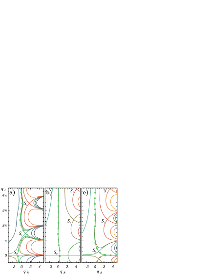
Figure 1: Equiphase paths in the complex plane, $w_{I}(q_{R},q_{I})=$ constant, with $w=\omega\Delta x^{2}$ and $q=k\Delta x$, for 3 values of the control parameter $\partial_{\phi}f_{2}(\phi_{m};{\mu})\Delta x^{2}=4$ (a), $-0.5$ (b), $-1$ (c). The saddles points $s_{i}$ are at the intersections between equiphase paths. The symbols show the steepest descent paths closing the integration contour.

In order to simplify the calculations, we define the parameters $\xi=\partial_{\phi}f_{1}(\phi_{m};{\mu})$, $\chi=\partial_{\phi}f_{2}(\phi_{m};{\mu})$. The analytic extension of the dispersion relation is $w=\xi\Delta x^{2}+q^{2}+\chi\Delta x^{2}e^{q}$, with $w=\omega\Delta x^{2}$ and $q=k\Delta x$, and we consider only the semi-plane $q_{I}\geq 0$ because $w(q)=w^{*}(q^{*})$. Note that the dispersion relation and the stability depend only upon the effective parameters $\xi\Delta x^{2}$ and $\chi^{\prime}\equiv\chi\Delta x^{2}$. For all values of $\chi^{\prime}$ there is at least a saddle and at most two saddles in the interval $q_{I}\in[0,\pi)$. We call the leftmost of these saddles $s_{0}$ (see Fig. 1b). For all $n>0$, there are also saddles $s_{n}$ in the $n$-th interval $q_{I}\in(2n\pi,(2n+1)\pi)$ for $\chi^{\prime}<0$ (Fig. 1b-c) or in the $n$-th interval $q_{I}\in((2n-1)\pi,2n\pi)$ for $\chi^{\prime}>0$ (Fig. 1a). In order to close the integration contour entirely with steepest descents, we need a steepest descent path that ends on or is asymptotic to the real axis ($q_{R}$) and another asymptotic to the imaginary axis ($q_{I}$). These steepest descents must either come from the same saddle or be connected by other steepest descents.

From the equation of the equiphase paths that originate at the saddle $s$, $2q_{I}q_{R}+\chi^{\prime}e^{q_{R}}\sin{q_{I}}=w_{I}(s)$, we can show that the possible asymptotes of the steepest descents are the imaginary axis for $q_{I}\rightarrow+\infty$ and the lines $q_{I}=(2n+1)\pi$ for $\chi^{\prime}>0$ and $n\geq 0$ (or the lines $q_{I}=2n\pi$ for $\chi^{\prime}<0$) and $q_{R}\rightarrow+\infty$. We determine the geometrical organisation of the steepest descents by using this information, together with the exact determination of the interception of the steepest descents with the lines $q_{I}=n\pi$ and with the imaginary axis and the fact that, in this problem, two steepest descents with different phases can intersect only at infinity Arfken . We find analytically that the saddle with the smallest phase $w_{I}$ ($s_{1}$ in Fig. 1a and $s_{0}$ in Fig. 1b and c) has always the upper steepest descent to the left of all the other steepest descents and asymptotic to the imaginary axis. Indeed this saddle is always necessary to close the integration contour. If $s_{0}$ happens to be the saddle with the smallest phase, then the steepest descents of $s_{0}$ close the integration contour (Fig. 1b-c) because $s_{0}$ either lies on the real axis or has another steepest descent asymptotic to the real axis. If instead there is another saddle $s_{n_{1}}$ with $w_{I}(s_{n_{1}})\leq w_{I}(s_{0})$ (for instance the saddle $s_{1}$ in Fig. 1a), than the upper steepest descent from $s_{0}$ remains below $s_{n_{1}}$ and is connected to the steepest descent from $s_{n_{1}}$ (in Fig. 1a these two steepest descents are asymptotically connected at $q_{I}=\pi$). In this case we use a steepest descent from $s_{n_{1}}$ to reach values of $q_{I}$ above $s_{n_{1}}$ itself and a steepest descent from $s_{0}$ to reach the real axis. If $s_{n_{1}}$ is the saddle with the smallest phase, then the steepest descents of $s_{0}$ and $s_{n_{1}}$ close the integration contour (symbol lines in Fig. 1a), otherwise we will have to include also the first saddle, $s_{n_{2}}$, with $n_{2}>n_{1}$ and $w_{I}(s_{n_{2}})\leq w_{I}(s_{n_{1}})$. In order to find the saddles to be used to close the integration contour, we repeat this process including all the saddles whose phase is the minimum of the phases of the saddles below them. For each finite $\chi^{\prime}$, this procedure gives a finite set of saddles $P_{\chi^{\prime}}$ . Examples of different integration contour are shown in Fig.(1) as symbols lines.

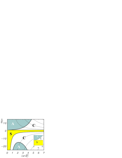
Figure 2: Instabilities diagram: Stable (S), convectively unstable (C) and absolutely unstable (A) regions for $\xi<0$. The dashed lines indicate where different bands become unstable. The insert shows the well-known diagram deissler obtained when instead of a non-local coupling a walk-off term ($v$) is considered. In this case there are no instabilities at all in the lower diagram region.

From Eq. (2) we identify the region $w_{R}(0,q_{I})<0$ in which the homogeneous solutions are stable. This is the region S in Fig. 2 and its contour is the convective threshold. If $w_{R}(0,q_{I})>0$ for some $q_{I}$ and if at least one saddle $s_{n}\in P_{\chi^{\prime}}$ has $w_{R}(s_{n})>0$, the instability is absolute. However, we need to find only a small subset of saddles in $P_{\chi^{\prime}}$ to determine the stability because $w_{R}(s_{n})>0$ only if there is instability with $w_{R}(0,q_{I})>0$ for $q_{I}$ in the $n$-th interval . Therefore, for each $\mu$, we can determine the nature of the instability by finding the values of $w$ at the saddles in $P_{\chi^{\prime}}$ that are in bands with instability threshold ${\chi^{\prime}}^{c}_{n}$ below the threshold ${\chi^{\prime}}^{a}_{0}$ where $w_{R}(s_{0})=0$. The absolute threshold $\chi^{\prime a}$ is then the value of $\chi^{\prime}$ where

$$\max\{w_{R}(s_{n})|s_{n}\in P_{\chi^{\prime}},{\chi^{\prime}}^{c}_{n}\leq{\chi^{\prime}}^{a}_{0}\}=0.$$ (3)

The importance of the determination of $P_{\chi^{\prime}}$ and of Eq. (3) is twofold. On one hand they guarantee that we can apply the method of steepest descents by properly closing the integration contour; on the other hand, they allow us to find the absolute threshold simply by inspection of $w$ at a finite number of saddles. This is remarkable in view of the infinite number of saddles produced by the shift. Moreover, $P_{\chi^{\prime}}$ is the same for all systems with the same $\chi^{\prime}$ in the class considered because the global geometrical organisation of the saddles and of their steepest descents does not depend on $\xi$.

Applying this technique we obtain the instabilities diagram in Fig. 2 valid for any $\xi\leq 0$ (including the typical case of a linear damping term $\xi=-1$). For $\chi<0$ the instability bands have $q_{I}\neq 0$ and the lowest convective threshold is very far from the absolute threshold. For $\chi>0$, the instability with respect to perturbations with $q_{I}=0$ is absolute for $\xi=0$ and convective for $\xi\neq 0$, with the convective instability windows increasing as $\xi$ decreases. Comparing the instabilities diagram for diffusive problems with finite shift and with with walk-off deissler (Fig. 2) we note that the whole $modulation$ instability region for negative values of $\chi$ is a specific effect of a finite shift, as was already recognised by ramazza98 . What our analysis reveals by direct calculation of the absolute threshold is that in this parameter region the system is mainly $convectively$ unstable and shows noise sustained modulated patterns. Only for very negative values of $\chi/|\xi|$ the absolute threshold is crossed.

Figure 3: a) $\chi_{0}(\mu)$ and $\chi_{\pm}(\mu)$ for the NGL equation. b) Gaussian perturbation (continuous line) of the vanishing state $\phi_{0}$ and evolved state for $\mu=1.03$ (dotted line) and for $\mu=1.09$ (dashed line). Shift $\Delta x=0.48$. The instability for $\mu=1.03$ is convective (local decay, even if the maximum of the perturbation grows), while for $\mu=1.09$ it is absolute (the perturbation grows also locally). After a longer transient the perturbation ends up colliding with the uniform stable states $\phi_{+}$ or $\phi_{-}$. Simulations with space discretization $0.12$, $4096$ grid points and time step $0.001$.

To show the general applicability of the stability analysis presented in this letter we consider in the following two examples: the Ginzburg-Landau and the saturable nonlinear equations, both with nonlocal nonlinear terms. A nonlocal Ginzburg-Landau (NGL) equation is obtained by Eq. (1) when

$$f_{1}=-\phi,~{}~{}~{}~{}f_{2}=\mu\phi-\phi^{3}.$$ (4)

The three uniform states $\phi_{0}=0$ (for any $\mu$) and $\phi_{\pm}=\pm\sqrt{\mu-1}$ (for $\mu>1$) are associated to the parameters $\xi_{0}=\xi_{\pm}=-1$ and $\chi_{0}=\mu$, $\chi_{\pm}=3-2\mu$ (Fig. 3a). Given the relation between $\chi_{0,\pm}$ and $\mu$, Fig. 2 provides the linear stability diagram of each state of the NGL equation. In particular, $\chi_{\pm}$ is always less than 1 so that only the lower part of the diagram in Fig. 2 describes $\phi_{\pm}$ instabilities, while for the state $\phi_{0}=0$ all the instabilities shown in the diagram arise by varying $\mu$ and the shift $\Delta x$. Without shift the state $\phi_{0}$ becomes unstable for $\mu>1$ where the system evolves to the homogeneous states $\phi_{+}$ and $\phi_{-}$(connected by fronts). With a finite shift for $\mu>1$ a region of convective instability arises before the absolute threshold. Simulations of the NGL equation with small values of $\mu$ show instabilities of the states $\phi_{0,\pm}$ in good agreement with our theoretical analysis. Fig. 3b is an illustrative example of the typical evolution of an initial perturbation of the unstable state $\phi_{0}$, below and above the predicted absolute threshold.

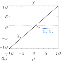
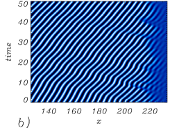
Figure 4: a) $\chi_{0}(\mu)$ and $\chi_{\pm}(\mu)$ for the AS equation. b) Noise sustained pattern for $\chi_{0}/|\xi|=\mu=-5$ and $\Delta x=1.92$ in the NAS with an additive Gaussian white noise of amplitude $0.01$. Simulations with Dirichlet boundary conditions and same numerical discretization of Fig. 3.

We now consider the nonlocal saturable nonlinear (NSN) equation obtained by Eq. (1) when

$$f_{1}=-\phi,~{}~{}~{}~{}f_{2}=\mu\frac{\phi}{1+\phi^{2}}.$$ (5)

We find the same three uniform states $\phi_{0}=0$, $\phi_{\pm}=\pm\sqrt{\mu-1}$ as before, but now $\chi_{0}=\mu$, $\chi_{\pm}=\frac{2-\mu}{\mu}$ (Fig. 4a). Again, knowing $\chi_{0,\pm}(\mu)$ and $\xi=-1$, Fig. 2 gives the thresholds of the NSN in terms of the specific parameters $\mu$ and $\Delta x$. We have seen before that for negative values of $\chi$ (here $\chi_{0}=\mu<0$) new modulation instabilities are predicted (both convective and absolute), existing $only$ for non-vanishing shifts and not observed in systems with drift. In Fig. 4b we show an example of a noise sustained stripe pattern, as predicted by our theoretical analysis.

The NSN equation has the advantage of not developing divergences even for large values of the control parameter due to the saturable nonlinearity. Therefore it was possible to check the instability diagram even for large negative values of $\chi_{0}$, decreasing $\mu$ from $-14$ to $-18$ (Fig. 5). Due to the modulational character of the instability an initial Gaussian perturbation does not evolves in the simple way shown in Fig. 3b. Nevertheless from the temporal evolution of the fronts it is still possible to distinguish without ambiguity between convective (Fig. 5a) and absolute (Fig. 5b) instabilities. It is also interesting to note that the wave-packet shows a clear asymmetry between the left and the right edges, with the wavenumbers with lower phase velocity in the leading edge and those with higher phase velocity in the trailing edge. This effect results from the symmetry breaking caused by the shift and the opposite sign of the group velocity and the phase velocities of most wavenumbers.

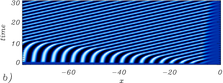
Figure 5: Temporal evolution of an initial Gaussian in $x=0$ perturbing the vanishing state $\phi_{0}$. a) For $\mu=-14$ the perturbation evolves toward a modulated wave-packet that eventually leaves the system (convective instability). b) For $\mu=-18$ the right front moves to the positive $x$ space region, and finally the modulated solution occupies the whole system (absolute instability). Simulation of the deterministic NSN equation with same parameters as in Fig. 4b.

In conclusion we have identified nonlocality as a new mechanism leading to convective instabilities in a large class of systems. We have shown how to determine the absolute threshold by finding the values of $w$ at a finite number of saddles which are selected out of an infinite number by the procedure described here. Our non perturbative approach allows us to analyse situations in which there are several bands of unstable wavenumbers and the absolute instability is very far from the lowest convective threshold. Theoretical predictions have been confirmed by numerical simulation of the dynamics of two prototype models. We expect that experiments in nonlocal systems will exhibit a dynamics dominated by noise and boundary effects in a very large region of control parameters. This opens the possibility of new and exciting research in the fundamental properties of extended nonlinear systems.

We acknowledge discussions with M. San Miguel, D. Walgraef and E. Yao. RZ is financially supported by the UK Engineering and Physical Sciences Research Council (GR/S03898/01).

References

- (1) J M. Chomaz, Phys. Rev. Lett. 69 1931 (1992); M. Santagiustina et al., Phys. Rev. Lett. 79 3633 (1997) Opt. Lett. 23, 1167 (1998); M. Taki et al., JOSA B 17, 997 (2000); R. Zambrini et al., Phys. Rev. A 65, 023813 (2002)
- (2) R. J. Briggs, Electron-Stream Interaction with Plasmas (MIT, Cambridge, MA, 1964)
- (3) K. L. Babcock, G. Ahlers, and D. S. Cannell, Phys. Rev. Lett. 67, 3388 (1991); P. Gondret et al., Phys. Rev. Lett. 82, 1442 (1999)
- (4) E. Louvergneaux et al., Phys. Rev. Lett. 93, 101801 (2004)
- (5) A.W. Snyder and D.J. Mitchel, Science 276, 1538 (1997); P. Cheben et al., Nature 408, 64 (2000)
- (6) P.L. Ramazza, S. Ducci, F.T. Arecchi, Phys. Rev. Lett. 81, 4128, (1998); S. Rankin, E. Yao and F. Papoff, Phys. Rev. A 68, 013821 (2003); L. Pastur, U. Bortolozzo, P.L. Ramazza, Phys. Rev. E 69, 016210 (2004)
- (7) J.P. Seipenbusch et al., Phys. Rev. A 56, R4401 (1997); Y. Hayasaki et al., Opt. Comm. 220, 281 (2003)
- (8) E. Infeld, G. Rowlands Nonlinear waves, solitons and chaos (Cambridge University Press, 1990)
- (9) C.M. Bender, S.A. Orszag, Advanced mathematical methods for scientists and engineers (Springer-Verlag, 1999)
- (10) G. Arfken, Mathematical Methods for Physicists, (Accademic Press, 1985)
- (11) R. J. Deissler, J. Stat. Phys. 40, 371 (1985)