Very fine structures in scalar mixing

Abstract

We explore very fine scales of scalar dissipation in turbulent mixing, below Kolmogorov and around Batchelor scales, by performing direct numerical simulations at much finer grid resolution than is usually adopted in the past. We consider the resolution in terms of a local, fluctuating Batchelor scale and study the effects on the tails of the probability density function and multifractal properties of the scalar dissipation. The origin and importance of these very fine-scale fluctuations are discussed. One conclusion is that they are unlikely to be related to the most intense dissipation events.

1 Introduction

Direct numerical simulations (DNS) of the equations governing turbulent phenomena have now become an important tool in both research and applications. Faithful results require the equations to be solved on a grid of adequate resolution. Most solutions of the past adopt a standard resolution based on an average measure of the smallest scale estimated from dimensional considerations. Our purpose here is to show, for the case of turbulent mixing, that such standard measures do not resolve a range of very fine scales that are present in reality. We demonstrate the essentials of this feature by performing several numerical simulations whose resolution is much finer than that adopted routinely, and comment on the practical relevance of the scales missed in past calculations.

We focus on the practically important case of $Sc\equiv\nu/\kappa>1$, where $Sc$ is the Schmidt number, $\nu$ the kinematic viscosity of the fluid and $\kappa$ the scalar diffusivity. The smallest scale of mixing is generated by the balance of turbulent stretching and diffusion (Batchelor 1959), and is related to the Kolmogorov scale $\overline{\eta}\equiv(\nu^{3}/\overline{\epsilon})^{1/4}$ through the identity $\overline{\eta}_{B}=\overline{\eta}/\sqrt{Sc}$; here, $\overline{\epsilon}$ is the average value of the instantaneous (and local) energy dissipation rate $\epsilon$ of the turbulent kinetic energy. The expression for $\epsilon$ reads as

$$\epsilon({\bf x},t) = \frac{\nu}{2}\sum_{i,j=1}^{3}\left(\frac{\partial u_{i}}{\partial x_{j}}+\frac{\partial u_{j}}{\partial x_{i}}\right)^{2},$$ (1)

where $u_{i}({\bf x},t)$ is the velocity fluctuation in the direction $i$. In simulations of a fixed size, in which the advection diffusion equation and the Navier-Stokes equations are simultaneously solved, the largest scale has traditionally been maximized by resolving no more than $\overline{\eta}_{B}$. Resolving this scale is also the goal of most experimental efforts, though they often fall short for large Péclet numbers $Pe\equiv u^{\prime}L/\kappa$, where $u^{\prime}$ and $L$, respectively, are the characteristic large-scale velocity and length scale of the flow.

However, since the time it was realized that the local energy dissipation rate $\epsilon$ has a multifractal character (e.g., Sreenivasan & Meneveau 1988), and that its average value $\overline{\epsilon}$ is therefore not adequate for quantifying small-scale characteristics (Grant, Stewart & Moilliet 1962), it has been clear that, locally, length scales smaller than $\overline{\eta}$ appear in a flow. This is obvious from the definition of the local Kolmogorov scale $\eta({\bf x},t)=(\nu^{3}/\epsilon({\bf x},t))^{1/4}$, in which $\epsilon({\bf x},t)$ is a highly fluctuating variable: the larger the value of $\epsilon$ locally, the smaller is the local Kolmogorov scale $\eta$, and vice versa. In view of the relation between the local values of the Batchelor and Kolmogorov scales, namely $\eta_{B}({\bf x},t)=\eta({\bf x},t)/\sqrt{Sc}$, it becomes similarly apparent that the existence of very small values of $\eta$ may lead to $\eta_{B}$ values that are much smaller than the average value $\overline{\eta}_{B}$. This intuitive (and incomplete) reasoning will be supplemented by further explanation momentarily, but it is enough to note here that such fine scales have not been explored before.

Section 2 presents a brief description of the simulations and resolution effects, and the main results are stated in section 3. This is followed by a discussion in section 4 of how the finest dissipation filaments are generated. Conclusions are stated in section 5.

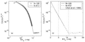
Figure 1: (a) Energy spectrum in the far-dissipation range for runs with $N=128$ and $N=512$, as indicated in the legend. In (b) we have fitted the data by $E(\tilde{k})\sim\tilde{k}^{\alpha}\exp(-c\tilde{k})$ where $\tilde{k}=k\overline{\eta}$, with $\alpha=3.3$ and $c=7.1$ as in Chen et al. (1993).

2 Resolution criteria and the far-dissipation range

The advection-diffusion equation for the passive scalar is solved together with the Navier-Stokes equations for the homogeneous and isotropic turbulent velocity field. The simulations are carried out within periodic boxes of fixed size $L^{3}=(2\pi)^{3}$. The flow is maintained stationary by a random volume forcing. The passive scalar is rendered stationary through a mean scalar gradient in the $y$-direction. Except for enhanced resolution, about which some comments follow, the pseudo-spectral methods used here are quite standard (Schumacher & Sreenivasan 2003; Vedula, Yeung & Fox 2001).

For DNS of box-type turbulence on an $N^{3}$ grid based on pseudo-spectral methods control of alias errors requires that modes with wavenumber higher than $k_{m}=\sqrt{2}N/3$ be truncated (Patterson & Orszag 1971). Specifically, this removes double and triple aliases in three dimensions. The usual resolution criterion is expressed as a number for $k_{m}\overline{\eta}$ which, by extension to cases with $Sc>1$, is

$$k_{m}\overline{\eta}_{B}\geq 1.5\,.$$ (2)

A proper resolution of the smallest scale requires that the global minimum of $\eta_{B}$ be resolved by the grid which can be written as

$$\frac{\min_{{\bf x},t}[\eta_{B}({\bf x},t)]}{\Delta}\geq 1\,.$$ (3)

By comparing (2.2) with the usual resolution criterion (2), we get

$$\frac{\overline{\eta}_{B}}{\Delta}\geq\frac{9}{4\sqrt{2}\pi}\approx 0.5\,,$$ (4)

where we used $\Delta=L/N=2\pi/N$ and $k_{m}=\sqrt{2}N/3$. It is apparent that the criterion (3) is stronger. Our simulation will satisfy (3) and its results will be compared with data from those with nominal grid resolution.

Unfortunately, the demands of this fine resolution restrict us to rather low values of the Reynolds number ($R_{\lambda}\leq 24$, see table 1 for details). This necessitates that most of our flow scales are in the viscous range of turbulence. Figure 1(a) shows the energy spectrum for $R_{\lambda}=10$, evaluated with two resolutions, $N=128$ and 512. It is seen that the noise floor is reached some 30 orders of magnitude below the peak signal. In figure 1(b), we verify that the energy spectrum in the far-dissipation range falls off as $E(\tilde{k})\sim\tilde{k}^{\alpha}\exp(-c\tilde{k})$ with $\tilde{k}=k\overline{\eta}$. For the lower Reynolds number case, one gets $\alpha=3.3$ and $c=7.1$ as did Chen et al. (1993) for the same range of dissipative wavenumbers; this range is indicated by the two vertical dotted lines in the figure.

$N^{3}$	$128^{3}$	$512^{3}$	$1024^{3}$
$R_{\lambda}=\sqrt{15/\nu\epsilon}\langle u_{x}^{2}\rangle$	10	10	24
$Sc$	32	32	32
$P_{\lambda}=Sc\,R_{\lambda}$	320	320	768
$L_{\theta}/L_{u}$	0.468	0.468	0.389
$T_{av}/T_{E}$	9.1	9.1	1.2
$k_{m}\overline{\eta}$	8.39	33.56	33.56
$k_{m}\overline{\eta}_{B}$	1.48	5.92	5.92
$\overline{\eta}_{B}/\Delta$	1/2	2	2
$\langle\theta^{2}\rangle^{1/2}$	2.57	2.57	1.91

Table 1: Parameters of the numerical simulations. $\Delta$ is the (equidistant) grid spacing. The integral length scale for the velocity field is $L_{u}=\pi/(2\overline{u_{x}^{2}})\int_{0}^{\infty}\mbox{d}kE(k)/k$ and that for the scalar field is $L_{\theta}=\pi/(2\overline{\theta^{2}})\int_{0}^{\infty}\mbox{d}kE_{\theta}(k)/k$; here $E(k)$ and $E_{\theta}(k)$ are the spectral densities of the velocity and scalar fields, respectively, $\overline{u_{x}^{2}}$ is the mean square of the velocity in the $x$-direction, and $\overline{\theta^{2}}$ that of the passive scalar. $T_{av}/T_{E}$ is the averaging time in units of the large scale eddy turnover time $T_{E}=3\overline{{u_{x}}^{2}}/2\overline{\epsilon}$.

3 Resolution effects on the scalar dissipation field

Figure 2 shows that the small scales of the scalar dissipation field $\epsilon_{\theta}$, defined by

$$\epsilon_{\theta}({\bf x},t) = 2\kappa\sum_{j=1}^{3}\left(\frac{\partial\theta}{\partial x_{j}}\right)^{2}\,,$$ (5)

appear as filamented structures in a planar cut. This is especially highlighted in the three-dimensional rendering of figure 3 which shows that very intense parts of scalar dissipation rate appear as sheets. Box counting of such events confirms a dimension close to 2. While no immediately discernible differences are apparent between the two scalar fields obtained with conventional and the present ultra-fine resolution (see the two upper panels of figure 2), the differences in $\epsilon_{\theta}$ can be detected more easily at several positions. This is seen quantitatively in figure 4, which shows that the resolution matters far away from the mean, or for the tails of the probability density function (PDF) of $\epsilon_{\theta}$. For $\epsilon_{\theta}\ll\overline{\epsilon_{\theta}}$, the PDF scales with an exponent of 1/2 and the curves for the two resolutions do not coincide. Significant differences in the large-amplitude tails ($\epsilon_{\theta}/\overline{\epsilon_{\theta}}>20$) are also apparent.

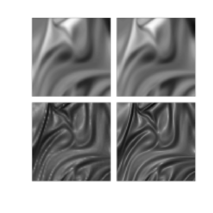
Figure 2: A slice in the ($x$-$z$) plane of the scalar field (upper row) and the corresponding scalar dissipation field (lower row in logarithmic units, black for maximum and white for minimum) at $Sc=32$ and $R_{\lambda}=10.$ Left column: low resolution case with $N=128$. Right column: high resolution case with $N=512$. A quarter of the plane is shown with an area of 131$\overline{\eta}_{B}\times 131\overline{\eta}_{B}$.

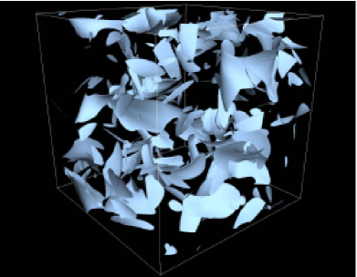
Figure 3: Isosurfaces of the scalar dissipation field for $R_{\lambda}=24$ and $Sc=32$. The level is $z\equiv\epsilon_{\theta}/\overline{\epsilon_{\theta}}=11$. Isosurfaces form flat and curved sheets which was also confirmed by a box counting analysis of isolevel sets.

An analytical result for the tails of $p(\epsilon_{\theta})$ exists for $Pe\to\infty$ in a smooth white-in-time flow. Using the Lagrangian approach, Chertkov, Falkovich & Kolokolov (1998) and Gamba & Kolokolov (1999) deduced the behaviour to be $p(\epsilon_{\theta})\sim\exp(-\epsilon_{\theta}^{1/3})$. Our finding here seems to be consistent with this result though our data are in the Eulerian frame.

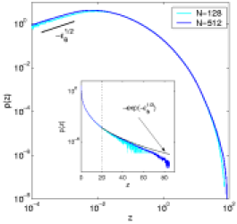
Figure 4: PDF $p(z)$ of the scalar dissipation field $z=\epsilon_{\theta}/\overline{\epsilon_{\theta}}$ for $N=128$ and $N=512$ at $Sc=32$. The outer panel shows the PDF in log-log scales while the inset shows a log-linear plot. The predicted tail behavior for a smooth white-in-time flow in the limit of $Pe\to\infty$ (Chertkov et al. 1998) is indicated in the inset. For the latter fit we included only the data with $z=\epsilon_{\theta}/\overline{\epsilon_{\theta}}>20$, as indicated by the dotted vertical line in the inset.

Another result that emphasizes the presence of very fine scales is shown in the left panel of figure 5 which plots, from three well-resolved simulations, the PDF of the local Batchelor scale $\eta_{B}({\bf x})=\eta({\bf x})/\sqrt{Sc}$ generated by mixing. The data for all three values of $Sc$ are advected in exactly the same flow. $\overline{\eta}_{B}$ is indicated for each $Sc$ by a vertical dashed line. It is clear that scales substantially smaller than $\overline{\eta}_{B}$ do exist, and that they are inaccessible to the standard resolution (2). The right panel of figure 5 illustrates that an increase of the Reynolds number will broaden the range of $\eta_{B}({\bf x})$ and thus magnifying the effect.

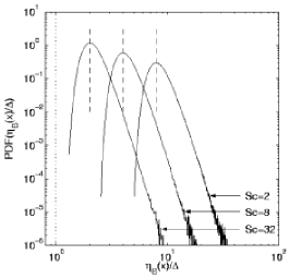
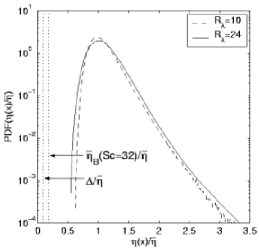
Figure 5: Left: Probability density function (PDF) of local fluctuations of the Batchelor scale in the mixing problem. The Taylor microscale Reynolds number is 10 and the Schmidt numbers are 2, 8, and 32. The computational domain is 512$\Delta$ on the side, where $\Delta$ is the grid spacing. The vertical dashed lines close to the maximum of each PDF indicates the average Batchelor scale $\overline{\eta}_{B}$. The dotted vertical line corresponds to one $\Delta$. Right: Reynolds number dependence of the fluctuations of the local dissipation scale, $\eta({\bf x})$. The Batchelor scale for $Sc=32$ and the grid spacing $\Delta$ are indicated by dotted lines. Since all lengths are rescaled by $\overline{\eta}$, both these parameters collapse for the two Reynolds numbers.

To highlight the sensitivity to fine-scale resolution, we have calculated the generalized dimensions

$$D_{q}(q)=\lim_{r\to 0}\frac{1}{q-1}\,\frac{\log\sum_{i}\mu_{i}^{q}(r)}{\log r}$$ (6)

where $r$ is the diameter of the subvolumes $B_{i}(r)$ of the successive coarse graining and the measure $\mu_{i}(r)=\overline{\epsilon_{\theta,\,B_{i}(r)}}/\overline{\epsilon_{\theta}}$ (Hentschel & Procaccia 1983). In the mid panel of figure 6 we compare the generalized dimensions for two runs, taking the same scaling range. Differences for $q<0$ are readily apparent. This part of the $D_{q}$ curve is dominated by low magnitudes of scalar dissipation. Clear differences are visible in the spatial distribution of regions of scalar dissipation below a certain small threshold value for the two runs (compare left and right panels). $D_{q}(q)$ for $q>0$ also shows differences, with the inadequately resolved data slightly underestimating the peak dissipation regions. Larger effects of inadequate resolution correspond to low amplitude regions rather than to high amplitude regions. They can be identified with wavenumbers $k>k^{\ast}$ where $k^{\ast}$ is the wavenumber at which the scalar dissipation spectrum $\epsilon_{\theta}(k)=2\kappa k^{2}E_{\theta}(k)$ peaks.

It is not surprising that poor resolution—which, in some sense, translates to increased noise—has a stronger effect on regions of low $\epsilon_{\theta}$ than those of high $\epsilon_{\theta}$ where the signal-to-noise ratio is effectively high.

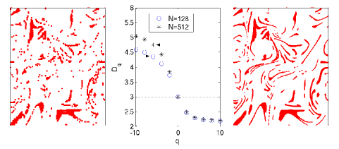
Figure 6: Generalized dimensions $D_{q}$ of the scalar dissipation field for nominal and ultra-fine resolutions. The values of $D_{q}$, shown on the left panel, were obtained by fits in the range $r\in[L/2^{6},L/2^{4}]$ with $L=2\pi$. The right panels show (without any additional numerical smoothing) slices through a snapshot for the data set $\epsilon_{\theta}/\overline{\epsilon_{\theta}}<0.025$ illustrating the differences in the calm regions that contribute to $D_{q}$ for $q<0$.

4 Scales of very high and very low scalar dissipation

We note that two different situations of large $Pe$ are of interest: (a) $Sc={\cal O}(1)$ at high Reynolds number and (b) $Sc\gg 1$ but at lower Reynolds numbers. In laboratory experiments dealing with liquid flows, the Reynolds numbers are moderate and the Schmidt numbers quite high (Sreenivasan 1991; Buch & Dahm 1996; Villermaux & Innocenti 1999; Catrakis et al. 2002). Most air experiments (Sreenivasan 1991a; Mydlarski & Warhaft 1998) are at higher Reynolds number and $Sc={\cal O}(1)$. Numerical simulations have considered either moderately high $Re$ and modest $Sc$ (Vedula, Yeung & Fox 2001; Watanabe & Gotoh 2004) or low $Re$ and large $Sc$ (Yeung, Xu & Sreenivasan 2002; Brethouwer, Hunt & Nieuwstadt 2003; Schumacher & Sreenivasan 2003; Yeung et al. 2004). Our situation is neither (a) nor (b) exactly, and we may expect small-scale scalar fluctuations influenced by the forcing which arises from velocity fluctuations.

The fluctuations of the velocity field around the Kolmogorov scale—in the intermediate dissipation range—have been discussed in Frisch & Vergassola (1991). A set of velocity increments, having a certain Hölder exponent $h$ in the inertial range—i.e. $\delta_{\ell}v\equiv|{\bf u}({\bf x}+{\bf\ell})-{\bf u}({\bf x})|\sim\ell^{h}$ with $\delta_{\ell}v$ being the velocity increment over a generic scale $\ell$ in the inertial range—and occupying a spatial support with a (fractal) dimension $D(h)$, is associated with a dissipation length $\eta(h)$. The “roughest” increments scale with $h_{min}$ and cause the largest spikes of energy dissipation persisting down to the smallest dissipative scale, $\eta(h_{min})$. The extent of the intermediate dissipation range is basically the width of the probability density functions as plotted in figure 5 (right). A global minimum of the local Batchelor scale would be given by the condition

$$\min_{{\bf x},t}[\eta_{B}({\bf x},t)]=\frac{\eta(h_{min})}{\sqrt{Sc}}\,,$$ (7)

which means that strongest scalar dissipation is controlled by $\eta(h_{min})=\nu^{3/4}/\max(\epsilon)$. To see if such a scale is related to the most intense scalar dissipation events, we estimate $\epsilon_{\theta}\sim\kappa\langle\theta^{2}\rangle/\ell^{2}$ by setting $\ell\equiv\eta(h_{min})/\sqrt{Sc}$ which is smaller than $\overline{\eta}_{B}$ and obtain

$$\max(\epsilon_{\theta})\simeq\overline{\theta^{2}}\,\sqrt{\frac{\max(\epsilon)}{\nu}}\,.$$ (8)

This connects directly the regions of high scalar dissipation to locations of large energy dissipation rate, as anticipated in section 1. Limitations of this expectation can be seen in figure 7, which plots the joint PDF, $p(\epsilon,\epsilon_{\theta})$. Large values of $\epsilon$ are not necessarily connected to large values of $\epsilon_{\theta}$. The crossing point of the dotted lines which is marked as a black square indicates that an extreme event as given by (8) is not present.

A second possibility is that the most intense scalar dissipation events are at scales in the viscous-convective range. Taking scalar increments $\delta_{\ell}\theta$ over this range, i.e. $\overline{\eta}_{B}<\ell<\overline{\eta}$, one gets due to Batchelor (1959) the expression

$$\overline{\delta_{\ell}\theta^{2}}=\overline{(\theta({\bf x}+{\bf\ell})-\theta({\bf x}))^{2}}\sim\overline{\epsilon_{\theta}}\sqrt{\frac{\nu}{\overline{\epsilon}}}\,\log\left(\frac{\ell}{\overline{\eta}_{B}}\right)\,.$$ (9)

A scale-dependent maximum of

$$\epsilon_{\theta}(\ell)\approx\kappa\frac{\overline{\delta_{\ell}\theta^{2}}}{\ell^{2}}\sim\kappa\overline{\epsilon_{\theta}}\sqrt{\frac{\nu}{\overline{\epsilon}}}\,\frac{\log(\ell/\overline{\eta}_{B})}{\ell^{2}}\$$ (10)

can be calculated via $\mbox{d}\epsilon_{\theta}(\ell)/\mbox{d}\ell=0$. This occurs at $\ell^{*}=\overline{\eta}_{B}\sqrt{\mbox{e}}$, which is larger than $\overline{\eta}_{B}$. The corresponding value $\epsilon_{\theta}(\ell^{*})$, shown by the dashed line, remains below the dotted horizontal line given by (8). The related scale is larger than the Batchelor scale which eases somewhat the strong resolution requirement (3).

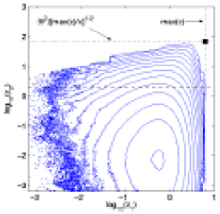
Figure 7: Joint PDF $p(z_{1},z_{2})$ with $z_{1}=\epsilon/\overline{\epsilon}$ and $z_{2}=\epsilon_{\theta}/\overline{\epsilon_{\theta}}$ for $N=512$. The contours are in equal increments of the logarithm to base 10, decreasing from 0.5 in steps of $-0.5$. The crossing point of the dotted lines is the maximum of $\epsilon_{\theta}$ following (8). The dashed line indicates the maximum if that maximum were to occur in the viscous-convective range.

	$R_{\lambda}=10$		$R_{\lambda}=24$
$\lambda_{k}=a_{k}\pm\mbox{i}b_{k}\;\;\;$	$z<10^{-3}$	$z>42\;\;\;\;\;$	$z<10^{-3}$	$z>69$	$z>42$	$z>11$
$(a_{1},a_{2},a_{3})$	$23\%$	$87\%$	$28\%$	$90\%$	$82\%$	$58\%$
$(a\pm\mbox{i}b,-2a)$	$77\%$	$13\%$	$72\%$	$10\%$	$18\%$	$42\%$

Table 2: Eigenvalue analysis of the velocity gradient tensor $\partial_{i}u_{j}$ at sites where $z=\epsilon_{\theta}/\overline{\epsilon_{\theta}}$ exceeds/falls below a threshold. The mean fraction of each of the possible eigenvalue solutions is given for two Reynolds numbers and a Schmidt number of 32. $\lambda_{1}+\lambda_{2}+\lambda_{3}=0$.

Of particular interest is the nature of the velocity field near the most intense or the least intense parts of the scalar dissipation. This was examined through the eigenvalue analysis of the velocity gradient at sites where $z=\epsilon_{\theta}/\overline{\epsilon_{\theta}}$ exceeded or fell below a chosen threshold. Trends with $Sc$ were discussed by Schumacher & Sreenivasan (2003), but here we focus only on the highest Schmidt number. The results of table 2 show that the pure straining motion (three real eigenvalues) and rotation (complex conjugated pair of eigenvalues) contribute to low amplitude scalar dissipation. It may be thought that the scale ${\ell}$ of maximum dissipation is related closely to the most compressive strain events, i.e. $\ell=\sqrt{\kappa/\max(|\gamma|)}$. The present data for all levels of $z$, some of which are reported in table 2, indicate that this is not so. Indeed, a broad range of compressive rates—not merely the maximal magnitudes—are associated with intense scalar dissipation. This is already apparent from the analysis of Ashurst et al. (1987) (see their figure 9b which reports an isotropic flow for Sc=0.5). While the most compressive eigenvector was preferentially aligned with the direction scalar gradient, corresponding events of maximum $\epsilon_{\theta}$ were preferentially aligned at an angle of about $20^{\circ}$. We explicitly note that this is the Eulerian point of view, and that a Lagrangian analysis following incipient fronts to the stage of their maturity may yield a different result.

5 Discussion

The possibility that the resolution requirement could be more stringent than is conventionally believed has been discussed to some detail in Sreenivasan (2004), but the details outlined in the present paper have not been explored before. When there is a significant overlap of the intermediate dissipation with the viscous-convective range, extreme values of the scalar dissipation are determined by the roughest velocity increments of the inertial range of turbulence. An important example in which these fine scales would make a difference is non-premixed turbulent combustion (Bilger 2004). There, the scalar dissipation rate of the mixture fraction enters as a basic quantity, e.g. for the modelling of jet-diffusion flames. Chemical reactions take place at the stochiometric mixture fraction in sheets of sub-Kolmogorov thickness. One expects steep gradients across such layers and strongly varying scalar dissipation. These variations are not captured in the flamelet equations where only the statistical mean enters the expansion parameter (Peters 2000).

A broad example where resolution effects can be important is the multifractal scaling of $\epsilon$ and $\epsilon_{\theta}$. The spiky structures in space and time, which are most prominent in the dissipative scales, are thought to affect appropriate turbulent field even for scales larger than $\eta$ or $\eta_{B}$, as appropriate (Frisch 1995).

To summarize, the very fine scalar filaments that were resolved here do not seem to be associated with the most intense scalar dissipation. The small-scale stirring in the flow seems to interrupt a further steepening process which is known as the formation of mature fronts. Similar findings were made for two-dimensional turblence at $Sc=1$ (Celani et al. 2001). Clearly, the Reynolds number of the advecting flow has an impact on this issue simply because the intermediate dissipation range might “overshadow” the viscous-convective range completely for sufficiently large $R_{\lambda}$. A more conclusive study of this issue will require higher Reynolds numbers and will be part of future work.

Computations were carried out using the NPACI resources provided by the San Diego Supercomputer Center and on the Jülich Multiprocessor (JUMP) IBM cluster at the John von Neumann-Institute for Computing, Jülich. Special thanks go to Herwig Zilken (Jülich) for his help with figure 3. PKY and KRS acknowledge support by the US National Science Foundation and JS from the Deutsche Forschungsgemeinschaft.

References

- (1) Ashurst, W. T., Kerstein, A. R., Kerr, R. M. & Gibson, C. H. 1987 Alignment of vorticity and scalar gradient with strain rate in simulated Navier-Stokes turbulence. Phys. Fluids 30, 2343-2353.
- (2) Batchelor, G. K. 1959 Small scale variation of convected quantities like temperature in a turbulent fluid. J. Fluid Mech. 5, 113-133.
- (3) Bilger, R. W. 2004 Some aspects of scalar dissipation. Flow Turb. Combust. 72, 93-114.
- (4) Brethouwer, G., Hunt, J. C. R. & Nieuwstadt, F. T. M. 2003 Micro-structure and Lagrangian statistics of the scalar field with a mean gradient in isotropic turbulence, J. Fluid Mech. 474, 193-225.
- (5) Buch, K. A. & Dahm, W. A. 1996 Experimental study of the fine-scale structure of conserved scalar mixing in turbulent shear flows. Part 1. , J. Fluid Mech. 317, 21-71.
- (6) Catrakis, H. J., Aguirre, R. C., Ruiz-Plancarte, J., Thayne, R. D., McDonald, B. A. & Hearn, J. W. 2002 Large-scale dynamics in turbulent mixing and the three-dimensional space-time behaviour of outer fluid interfaces. J. Fluid Mech. 471, 381-408.
- (7) Celani, A., Lanotte, A., Mazzino, A. & Vergassola, M. 2001 Fronts in scalar turbulence. Phys. Fluids 13, 1768-1783.
- (8) Chen, S., Doolen, G., Herring, J. R., Kraichnan, R. H., Orszag, S. A. & She, Z.-S. 1993 Far-dissipation range of turbulence. Phys. Rev. Lett. 70, 3051-3054.
- (9) Chertkov, M., Falkovich, G. & Kolokolov, I. 1998 Intermittent dissipation of a passive scalar in turbulence. Phys. Rev. Lett. 80, 2121-2124.
- (10) Frisch, U. & Vergassola, M. 1991 A prediction of the multifractal model: the intermediate dissipation range. Europhys. Lett. 14, 439-444.
- (11) Frisch, U. 1995 Turbulence, Cambridge: Cambridge University Press.
- (12) Gamba, A. & Kolokolov, I. 1999 Dissipation statistics of a passive scalar in a multi-dimensional smooth flow. J. Stat. Phys. 94, 759-777.
- Grant, Stewart & Moilliet, (1962) Grant, H. L., Stewart, R. W. & Moilliet, A. 1962 Turbulence spectra from a tidal channel. J. Fluid. Mech. 12 241-268.
- Procaccia (1983) Hentschel, H. G. E. & Procaccia, I. 1983 The infinite number of generalized dimensions of fractals and strange attractors. Physica D 8, 435-444.
- Mydlarski (1998) Mydlarski, L. & Warhaft, Z. 1998 Passive scalar statistics in high-Peclet-number grid turbulence. J. Fluid Mech. 358, 135-175.
- (16) Patterson, G. S. & Orszag, S. A. 1971 Spectral calculations of isotropic turbulence: efficient removal of aliasing interactions. Phys. Fluids 14, 2538-2541.
- Peters (2000) Peters, N. 2000 Turbulent Combustion, Cambridge: Cambridge University Press.
- Schumacher & Sreenivasan (2003) Schumacher, J. & Sreenivasan, K. R. 2003 Geometric features of the mixing of passive scalars at high Schmidt numbers. Phys. Rev. Lett. 91, 174501 (4 pages).
- Sreenivasan & Meneveau, (1988) Sreenivasan, K. R. & Meneveau, C. 1988 Singularities of the equations of motion. Phys. Rev. A 38 6287-6295.
- Sreenivasan (1991) Sreenivasan, K. R. 1991 Fractals and multifractals in fluid turbulence. Annu. Rev. Fluid Mech. 23, 539-600.
- Sreenivasan (1991a) Sreenivasan, K. R. 1991a On local isotropy of passive scalars in turbulent shear flows. Proc. Roy. Soc. A434, 165-182.
- Sreenivasan (2004) Sreenivasan, K. R. 2004 Possible effects of small-scale intermittency in turbulent reacting flows. Flow Turb. Combust. 72, 115-141.
- Vedula, Yeung & Fox (2001) Vedula, P., Yeung, P. K. & Fox, R. O. 2001 Dynamics of scalar dissipation in isotropic turbulence: a numerical and modelling study. J. Fluid Mech. 433, 29-60.
- Villermaux (1999) Villermaux, E. & Innocenti, C. 1999 On the geometry of turbulent mixing. J. Fluid Mech. 393, 123-148.
- Watanabe (2004) Watanabe, T. & Gotoh, T. 2004 Statistics of passive scalar in homogeneous turbulence. New J. Phys. 6, 40 (36 pages).
- Yeung (2002) Yeung, P. K., Xu, S. & Sreenivasan, K. R. 2002 Schmidt number effects on turbulent transport with uniform mean scalar gradient. Phys. Fluids 14, 4178-4191.
- (27) Yeung, P.K., Xu, S., Donzis, D.A. & Sreenivasan, K.R. 2004 Simulations of three-dimensional turbulent mixing at Schmidt numbers of the order 1000. Flow Turb. Combust. 72, 333-347.