Second order additive invariants in elementary cellular automata

1 Introduction

Cellular automata (CA) are often described as systems of cells in a regular lattice updated synchronously according to a local interaction rule. An interesting subclass of CA consists of rules possessing an additive invariant. The simplest of such invariants is the total number of sites in a particular state. CA with such invariant, often called “conservative CA” or “number-conserving CA”, generated a lot of interest in recent years [1, 2, 3, 4, 5]. Number-conserving CA can be viewed as a system of interacting and moving particles, where in the case of a binary rule, 1’s represent sites occupied by particles, and 0’s represent empty sites. The flux or current of particles in equilibrium depends only on their density, which is invariant. The graph of the current as a function of density characterizes many features of the flow, and is therefore called the fundamental diagram.

For a majority of number-conserving CA rules, fundamental diagrams are piecewise-linear, usually possessing one or more “sharp corners” or singularities. There exist a strong evidence of universal behavior at singularities, as reported in [6, 7].

Since number-conserving CA are simplest rules with additive invariants, it would be interesting to consider higher order invariants and CA rules with such invariants. In 1991, Hattori and Takesue performed extensive study of additive invariants in discrete-time lattice dynamical systems [8], not necessarily restricted to CA. They derived very general existence conditions, and applied them to elementary CA rules as well as reversible CA. In this paper, we will use their results to study second-order invariants in elementary rules, focusing mainly on fundamental diagrams.

2 Number-conserving cellular automata

In what follows, we will assume that the dynamics takes place on one-dimensional lattice of length $L$ with periodic boundary conditions. Let $s_{i}(t)$ denote the state of the lattice site $i$ at time $t$, where $i\in\{0,1,\ldots,L-1\}$, $t\in\mathbbm{N}$. All operations on spatial indices $i$ are assumed to be modulo $L$. We will further assume that $s_{i}(t)\in\{0,1\}$, and we will say that the site $i$ is occupied (empty) at time $t$ if $s_{i}(t)=1$ ($s_{i}(t)=0$).

Let $l$ and $r$ be two integers such that $l\leq 0\leq r$, and let $n=r-l+1$. The set $\{s_{i+l}(t),s_{i+l+1}(t),\ldots,s_{i+r}(t)\}$ will be called the neighbourhood of the site $s_{i}(t)$. Let $f$ be a function $f:\{0,1\}^{n}\rightarrow\{0,1\}$, also called a local function The update rule for the cellular automaton is given by

$$s_{i}(t+1)=f(s_{i+l}(t),s_{i+l+1}(t),\ldots,s_{i+r}(t)).$$ (1)

In [8], the concept of additive invariant for CA has been introduced. Let $\alpha$ be a non-negative integer, and let $\xi=\xi(x_{0},x_{1},\ldots,x_{\alpha})$ be a function of $\alpha+1$ variables taking values in ${\mathbbm{R}}$. We say that $\xi$ is a density function of an additive conserved quantity if for every positive integer $L$ and for every initial condition $(s_{0}(0),s_{1}(0),\ldots,s_{L-1}(0))\in\{0,1\}^{L}$ we have

$$\sum_{i=0}^{L-1}\xi(s_{i}(t),s_{i+1}(t),\ldots,s_{i+\alpha}(t))=\sum_{i=0}^{L-1}\xi(s_{i}(t+1),s_{i+1}(t+1),\ldots,s_{i+\alpha}(t+1))$$ (2)

for all $t\in{\mathbbm{N}}$. For simplicity, if the above condition is satisfied, we will say that $\xi$ is an additive invariant of $f$. It is often more convenient to write (2) using the function $G$ defined as

$$G(x_{0},x_{1},\ldots,x_{\alpha+n-1})=\xi(f(x_{0},x_{1},\ldots,x_{n-1}),f(x_{1},x_{2},\ldots,x_{n}),\ldots,f(x_{\alpha},x_{\alpha+1},\ldots,x_{\alpha+n-1})).$$ (3)

With this notation, $\xi$ is an additive invariant of $f$ if

$$\sum_{i=0}^{L-1}G(x_{i},x_{i+1},\ldots,x_{i+\alpha+n-1})=\sum_{i=0}^{L-1}\xi(x_{i},x_{i+1},\ldots,x_{i+\alpha})$$ (4)

for every positive integer $L$ and for all $x_{0},x_{1},\ldots,x_{L-1}\in\{0,1\}$.

In recent years, many authors studied the case of the simplest additive invariant, with $\alpha=0$ and $\xi(x_{0})=x_{0}$. For this invariant, the equation (2) becomes

$$\sum_{i=0}^{L-1}s_{i}(t)=\sum_{i=0}^{L-1}s_{i}(t+1),$$ (5)

which means that the CA rule posessing this invariant conserves the number of sites in state 1. Such rules are often referred to as number-conserving rules. Among elementary CA, i.e. those with $l=-1$ and $r=1$, there are only five number-conserving rules. Three of these are trivial, namely the identity rule 204 and two shifts 170 and 240. Two remaining rules, 184 and 226, are equivalent under the spatial reflection. Rule 184, which is a discrete version of the totally asymmetric exclusion process, has been extensively studied [9, 10, 11, 12, 13, 14, 15, 16], and many rigorous result regarding its dynamics have been established.

Hattori and Takesue [8] established a very general result which we will write here in a somewhat simplified form, taking into account that this paper is concerned with binary rules only.

Theorem 1 (Hattori & Takesue ’91)

Let $\xi(x_{0},x_{1},\ldots,x_{\alpha})$ be a function of $\alpha+1$ variables. Then $\xi$ is a density function of an additive conserved quantity under the time evolution of cellular automaton rule (1) if and only if the condition

$$G(x_{0},x_{1},\ldots,x_{\alpha+n-1})-\xi(x_{-l},x_{-l+1},\ldots,x_{\alpha-l})=J(x_{0},x_{1},\ldots,x_{\alpha+n-2})-J(x_{1},x_{2},\ldots,x_{\alpha+n-1})$$ (6)

holds for all $x_{0}$, $x_{1}$, $\ldots$, $x_{\alpha+n-1}\in\{0,1\}$, where the quantity $J$, to be referred to as the current, is defined by

$$J(x_{0},x_{1},\ldots,x_{\alpha+n-2})=-\sum_{i=0}^{\alpha+n-2}G(\overbrace{0,0,\ldots,0}^{\alpha+n-1-i},x_{0},x_{1},\ldots,x_{i})+\sum_{i=-l-n+2}^{\alpha-l}\xi(\overbrace{0,0,\ldots,0}^{\alpha+1-i},x_{0},x_{1},\ldots,x_{i-1}).$$ (7)

The following convention is used in the definition of $J$:

$$\xi(\overbrace{0,0,\ldots,0}^{\alpha+1-i},x_{0},x_{1},\ldots,x_{i-1})=\xi(x_{i-\alpha-1},x_{i-\alpha},\ldots,x_{i-1})\mbox{\,\,\,\,\,if $i\geq\alpha+1$},$$ (8)

and

$$\xi(\overbrace{0,0,\ldots,0}^{\alpha+1-i},x_{0},x_{1},\ldots,x_{i-1})=\xi(0,0,\ldots,0)\mbox{\,\,\,\,\,if $i\leq 0$}.$$ (9)

The equation (6) can be interpreted in a similar way as a conservation law in a continuous, one dimensional physical system. In such system, let $\rho(x,t)$ denote the density of some material at point $x$ and time $t$, and let $j(x,t)$ be the current (flux) of this material at point $x$ and time $t$. A conservation law states that the rate of change of the total amount of material contained in a fixed domain is equal to the flux of that material across the surface of the domain. The differential form of this condition can be written as

$$\frac{\partial\rho}{\partial t}=-\frac{\partial j}{\partial x}.$$ (10)

Since in our case $\xi$ is the the density of an additive conserved quantity, the left hand side of (6) is simply the change of density in a single time step, so that (6) is an obvious discrete analog of the current conservation law (10) with $J$ playing the role of the current.

Let us now assume that the initial configuration has been generated from some translation-invariant distribution $\mu$. We define the expected value of $\xi$ at site $i$ as

$$\rho(i,t)=E_{\mu}\left[\xi(s_{i}(t),s_{i+1}(t),\ldots,s_{i+\alpha}(t))\right].$$ (11)

Since the initial distribution is $i$-independent, we expect that $\rho(i,t)$ also does not depend on $i$, and we will therefore define $\rho(t)=\rho(i,t)$. Furthermore, since $\xi$ is density function of a conserved quantity, $\rho(t)$ is $t$-independent, so we define $\rho=\rho(t)$. The expected value of the current $J(s_{i+l}(t),s_{i+l+1}(t),\ldots,s_{i+r-1}(t))$ will also be $i$-independent, so we can define the expected current as

$$j(\rho,t)=E_{\mu}\big{(}J(s_{i+l}(t),s_{i+l+1}(t),\ldots,s_{i+r-1}(t))\big{)}.$$ (12)

The graph of the equilibrium current $j(\rho,\infty)=\lim_{t\rightarrow\infty}j(\rho,t)$ versus the density $\rho$ is known as the fundamental diagram.

3 Number-conserving nearest-neighbour rules

In order to illustrate the theorem of the previous section, we will first consider the case of number-conserving nearest-neighbour rules, i.e., $\alpha=0$ and $\xi(x_{0})=x_{0}$, $l=-1$, $n=3$. Condition (6) becomes

$$G(x_{0},x_{1},x_{2})-\xi(x_{1})=J(x_{0},x_{1})-J(x_{1},x_{2}),$$ (13)

where

$$J(x_{0},x_{1})==-G(0,0,x_{0})-G(0,x_{0},x_{1})+\xi(0)+\xi(x_{0})$$ (14)

Obviously, $G(x_{0},x_{1},x_{2})=f(x_{0},x_{1},x_{2})$, thus the current becomes $J(x_{0},x_{1})=-f(0,0,x_{0})-f(0,x_{0},x_{1})-x_{0}$, and the conservation condition takes the form

$$f(x_{0},x_{1},x_{2})-x_{1}=J(x_{0},x_{1})-J(x_{1},x_{2}).$$ (15)

As mentioned earlier, rule 184 and its spatial reflection are the only non-trivial elementary CA rules satisfying (15). For rule 184, $f$ is defined by $f(x_{0},x_{1},x_{2})=x_{0}-x_{0}x_{1}+x_{1}x_{2}$ and the current can be written as $J(x_{0},x_{1})=x_{0}(1-x_{1})$. It is possible to show [13] that the equilibrium current for this rule is given by

$$j(\rho,\infty)=\left\{\begin{array}[]{ll}\rho&\mbox{if $\rho<1/2$},\\ 1-\rho&\mbox{otherwise}.\end{array}\right.$$ (16)

Since number-conserving CA rules conserve the number of occupied sites, we can label each occupied site (or “particle”) with an integer $k\in\mathbbm{Z}$, such that the closest particle to the right of particle $k$ is labeled $k+1$. If $y_{k}(t)$ denotes the position of particle $k$ at time $t$, the configuration of the particle system at time $t$ is described by the increasing bisequence $\{y_{k}(t)\}_{k=-\infty}^{\infty}$. We can then specify how the position of the particle at the time step $t+1$ depends on positions of the particle and its neighbours at the time step $t$. For example, for rule 184 one obtains

$$y_{k}(t+1)=y_{n}(t)+\min\{y_{k+1}(t)-y_{k}(t)-1,1\}.$$ (17)

Equation (17) is sometimes referred to as the motion representation. The motion representation is analogous to Lagrange representation of the fluid flow, in which we observe individual particles and follow their trajectories [17]. It turns out that the motion representation can be constructed for arbitrary number-conserving CA rule by employing algorithm described in [18].

4 Second-order invariants

In what follows, we will referr to the number of variables of $\xi$ as the order of the invariant, equal to $\alpha+1$. Since the invariant of $\alpha=0$ and corresponding fundamental diagrams have been extensively studied, we will explore the case of $\alpha=1$, i.e., second order invariants, using the method of [8].

The arguments $x_{0},x_{1}$ of the density function take values in the set $\{0,1\}$, and therefore $\xi$ can be defined in terms of four parameters

$$\xi(0,0)=c_{00},\,\,\xi(0,1)=c_{01},\,\,\xi(1,0)=c_{10},\,\,\xi(1,1)=c_{11},$$ (18)

where $c_{00},c_{01},c_{10},c_{11}\in\mathbbm{R}$. This can be also expressed as

$$\xi(x_{0},x_{1})=c_{00}(1-x_{0})(1-x_{1})+c_{01}(1-x_{0})x_{1}+c_{10}x_{0}(1-x_{1})+c_{11}x_{0}x_{1}$$

$$=c_{00}+(c_{10}-c_{00})x_{0}+(c_{01}-c_{00})x_{1}+(c_{00}-c_{01}-c_{10}+c_{11})x_{0}x_{1}.$$

The constant term does not bring anything new, so we can set $c_{00}=0$. Moreover, note that for any function $g(x)$ and any $x_{0},x_{1},\ldots,x_{L-1}\in\{0,1\}$ we have

$$\sum_{i=0}^{L-1}\xi(x_{i},x_{i+1})=\sum_{i=0}^{L-1}\big{(}\xi(x_{i},x_{i+1})+g(x_{i})-g(x_{i+1})\big{)},$$ (19)

which means that if $\xi(x_{0},x_{1})$ is a density function of some conserved additive quantity, then $\widehat{F}(x_{0},x_{1})=\xi(x_{0},x_{1})+g(x_{0})-g(x_{1})$ is also a density function of a conserved additive quantity. To remove this ambiguity, we will require that $\xi(0,x_{1})=0$, similarly as done in [8]. This yields $c_{01}=0$, and we are left with $\xi$ depending on two parameters only

$$\xi(x_{0},x_{1})=c_{10}x_{0}+(c_{11}-c_{10})x_{0}x_{1}.$$ (20)

Defining $a_{1}=-c_{10}$, $a_{2}=c_{11}-c_{10}$, we arrive at the final parameterization of $\xi$

$$\xi(x_{0},x_{1})=a_{1}x_{0}+a_{2}x_{0}x_{1},\mbox{\,\,\,}a_{1},a_{2}\in\mathbbm{R}.$$ (21)

For $\alpha=1$, $l=-1$, and $n=3$, eq. (6) becomes

$$G(x_{0},x_{1},x_{2},x_{3})-\xi(x_{1},x_{2})=J(x_{0},x_{1},x_{2})-J(x_{1},x_{2},x_{3}),$$ (22)

where

$$G(x_{0},x_{1},x_{2},x_{3}) = \xi(f(x_{0},x_{1},x_{2}),f(x_{1},x_{2},x_{3}))$$

$$J(x_{0},x_{1},x_{2}) = -G(0,0,0,x_{0})-G(0,0,x_{0},x_{1})-G(0,x_{0},x_{1},x_{2})$$

$$\mbox{\,}+\xi(0,0)+\xi(0,x_{0})+\xi(x_{0},x_{1}).$$

Since $\xi(0,0)=\xi(0,x_{0})=0$, the formula for current simplifies to

$$J(x_{0},x_{1},x_{2})=-G(0,0,0,x_{0})-G(0,0,x_{0},x_{1})-G(0,x_{0},x_{1},x_{2})+\xi(x_{0},x_{1}).$$ (23)

For a given elementary CA rule $f(x_{0},x_{1},x_{2})$, one can write eq. (22) for all $2^{4}$ combinations of values of the variables $x_{0},x_{1},x_{2},x_{3}\in\{0,1\}$, thus obtaining an overdetermined linear system of 16 equations with two unknowns $a_{1},a_{2}$. This system is homogeneous, therefore the solution, if it exists, is not unique. That is, if $(a_{1},a_{2})$ is a solution, then $(ca_{1},ca_{2})$ is also a solution for any $c\in\mathbbm{R}$. We will normalize the solution so that the first non-zero number in the pair $(a_{1},a_{2})$ is set to be equal to 1.

Solving these equations for all “minimal” CA rules, one finds that for most CA rules solutions do not exist. Remaining CA rules can be divided into two classes. The first class contains rules 204 and 170, and for these rules, any pair $(a_{1},a_{2})$ is a solution. We will not be concerned with these rules, since they exhibit trivial dynamics. The second class consists of 10 rules for which a unique solution exists (up to the normalization described earlier). These rules are 12, 14, 15, 34, 35, 42, 43, 51, 140, 142, and 200, as reported in [8].

Table 1 shows the density function $\xi$ and the current $J$ for all of them. The formulas for the current have been obtained using the HCELL C++ library for cellular automata developed by the author.

Rule number	$\xi(x_{0},x_{1},x_{2})$	$J(x_{0},x_{1})$
12	$x_{0}-x_{0}x_{1}$	$-x_{0}x_{1}$
14	$x_{0}-x_{0}x_{1}$	$-x_{0}x_{1}$
15	$x_{0}-x_{0}x_{1}$	$-x_{0}x_{1}$
34	$x_{0}-x_{0}x_{1}$	$-x_{1}$
35	$x_{0}-x_{0}x_{1}$	$-x_{1}$
42	$x_{0}-x_{0}x_{1}$	$-x_{1}+x_{1}x_{2}-x_{0}x_{1}x_{2}$
43	$x_{0}-x_{0}x_{1}$	$-x_{1}+x_{1}x_{2}-x_{0}x_{1}x_{2}$
51	$x_{0}-x_{0}x_{1}$	$-x_{1}$
140	$x_{0}-x_{0}x_{1}$	$-x_{0}x_{1}+x_{0}x_{1}x_{2}$
142	$x_{0}-x_{0}x_{1}$	$-x_{0}x_{1}+x_{0}x_{1}x_{2}$
200	$x_{0}x_{1}$	$0$

Table 1: Density of the invariant $\xi$ and the current $J$ for all non-trivial elementary CA with second order invariants.

5 Fundamental diagrams

In order to construct fundamental diagrams for rules of Table 1, we first note that the current for rule 200 is identically equal to zero, thus the equilibrium current $j(\rho,\infty)=0$. The graph of $j(\rho,\infty)$ vs. $\rho$ for this rule is, therefore, not interesting.

For all other rules, the density of the invariant is given by the same function $\xi(x_{0},x_{1})=x_{0}-x_{0}x_{1}$. This means that rules 12, 14, 15, 34, 35, 42, 43, 51, 140, and 142 conserve the number of blocks “10” in the configuration. In order to construct their fundamental diagrams, we have to be able to create an initial configuration with a given number of pairs “10”. Construction of a configuration of length $L$ with exactly $m$ pairs “10” can proceed according to the following algorithm. We start with an array of $L$ integers, $\{s_{i}(0)\}_{i=0}^{L-1}$.

1. Set $s_{i}(0)=0$ for all $i=0,1,\ldots,L-1$.

2. Place the symbol “C” at randomly selected site of the array. Then place another symbol “C” at another site randomly selected among all remaining empty sites. Repeat this procedure until you place exactly $2m$ symbols “C”.

3. Let $x=0$. Starting from $i=0$, traverse the array filling it with $x$ values. Every time when you encounter $C$, set $x:=1-x$. Stop when you reach the end of the array.

The average density of the invariant $\xi(x_{0},x_{1})=x_{0}-x_{0}x_{1}$ for the configuration obtained with the above algorithm will be

$$\rho_{av}=\frac{1}{L}\sum_{i=0}^{L-1}\xi(s_{i}(t),s_{i+1}(t))=\frac{m}{L},$$ (24)

and it will be independent of $t$. We can also define average current at time $t$ for a configuration with average density $\rho_{av}$ of the invariant as

$$j_{av}(\rho_{av},t)=\frac{1}{L}\sum_{i=0}^{L-1}J(s_{i}(t),s_{i+1}(t),s_{i+2}(t)).$$ (25)

Graph of $j_{av}(\rho_{av},t)$ vs. $\rho_{av}$ for very large $t$ will approximate the graph of $j(\rho,\infty)$ (given by eq. 12) vs. $\rho$, i.e., the fundamental diagram.

For six rules from Table 1, the fundamental diagram is strictly linear, and the following expressions for current can be conjectured based on numerical experiments.

$$\mbox{Rule 12:\,\, }j(\rho,\infty) = 0$$

$$\mbox{Rule 15:\,\, }j(\rho,\infty) = \rho-1/2$$

$$\mbox{Rule 34:\,\, }j(\rho,\infty) = -\rho$$

$$\mbox{Rule 42:\,\, }j(\rho,\infty) = -\rho$$

$$\mbox{Rule 51:\,\, }j(\rho,\infty) = -1/2$$

$$\mbox{Rule 140:\,\, }j(\rho,\infty) = 0$$

The remaining four rules are more interesting, as they exhibit singularities in fundamental diagrams, as shown in Figure 1.

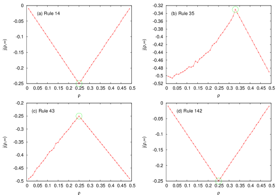
Figure 1: Fundamental diagrams for rules 14, 35, 43, 142. Singularities are denoted by green circles. Diagrams have been obtained using 50000 lattice sites after 50000 iterations.

It is remarkable that singularities are present only in fundamental diagram of those particular rules. In [8], authors searched for invariants of up to seventh order for all “minimal” elementary CA. According to the table published in their paper, rules $14,35,43,142$ do not have any other invariant except $\xi(x_{0},x_{1})=x_{0}-x_{0}x_{1}$, in contrast to remaining rules of Table 1, which also posses other higher order invariants. It seems that singularities in the fundamental diagram can appear only in rules which have only one invariant, just like rule 184, which only has first order invariant $\xi(x_{0})=x_{0}$.

6 Convergence to equilibrium

In number-conserving cellular automata, singularities of the fundamental diagram exhibit critical behavior. This can be illustrated by introducing the the decay time defined as

$$\tau(\rho)=\sum_{t=0}^{\infty}|j(\rho,t)-j(\rho,\infty)|.$$ (26)

If the decay of $j(\rho,t)$ toward its equilibrium value $j(\rho,\infty)$ is of power-law type, the above sum diverges. For all rules in Figure 1, we have performed computer simulations to estimate $\tau$. The value of $\tau$ has been estimated by measuring $j_{av}(\rho,t)$ for $t=0,1,\ldots,1000$, and truncating the sum (26) at $t=1000$. Figure 2 shows a typical graph of $\tau$ as a function of $\rho$, obtained for rule 42. Comparing Figures 1c and Figure 2 we clearly see that $\tau$ diverges at the critical point of rule 42, which occurs at $\rho=0.25$. We will denote this value by $\rho_{c}$.

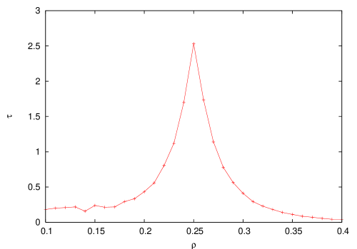
Figure 2: Decay time vs. density of the invariant for rule 43.

Assuming that $|j(\rho_{c},\infty)-j(\rho_{c},t)|\sim t^{-\alpha}$, we have determined the exponent $\alpha$ as the slope of the straight line which best fits the logarithmic plot of $|j(\rho_{c},\infty)-j(\rho_{c},t)|$ vs. time $t$. Example of such a plot, again for rule 42, is shown in Figure 3. Table 2 shows values of the exponent $\alpha$ for critical points of all four rules of Figure 1.

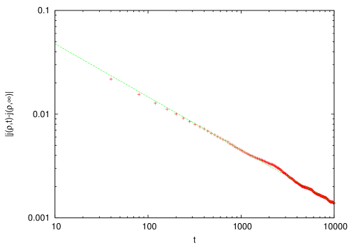
Figure 3: Logarithmic plot of $|j(\rho_{c},\infty)-j(\rho_{c},t)|$ as a function of time for rule 43. Data points ($+$) represent computer simulations, while the dashed line represents the best fit.

Rule number	$(\rho_{c},j(\rho_{c},\infty))$	$\alpha$
14	$(1/4,-1/4)$	$-0.504$
35	$(1/3,-1/3)$	$-0.472$
43	$(1/4,-1/4)$	$-0.492$
142	$(1/4,-1/4)$	$-0.502$

Table 2: Values of the exponent $\alpha$ at the critical point for elementary CA rules with second-order additive invariant.

Exponent $\alpha$ is known to be equal to exactly $1/2$ for rule 184 and its generalizations, and rigorous proof of this fact exists [13]. Extensive numerical experiments support the conjecture that for all rules with first-order invariant the value $\tau=1/2$ is universal, in the case of both piecewise linear [6] and nonlinear [6] fundamental diagrams. Table 2 provides evidence that a more general conjecture may be valid: regardless of the order of the invariant, exponent $\alpha$ seems to have universal value of $1/2$. In the next section we will offer some justification for this conjecture for rules with second-order invariants.

7 Dynamics of localized structures

In rule 184, the power-law convergence of the current toward its equilibrium value is related to the dynamics of this rule, which resembles ballistic annihilation. The spatiotemporal patter generated by rule 184 can be understood as propagation of two types of localized structures, shown in Figure 4.

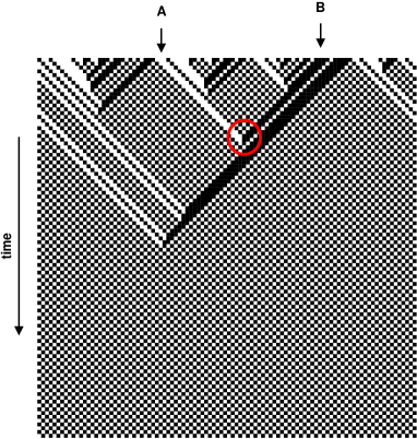
Figure 4: Spatiotemporal pattern generated by rule 184. Initial configuration is represented by the top row, where black squares represent 1’s, and white spaces represent 0’s. Consecutive configurations are plotted as consecutive rows. Two types of defects of “A” and “B” type are visible, annihilating in the circled spot.

These two types of structures, marked with letters “A” and “B”, propagate in opposite directions and annihilate upon collision. At the critical point, the number of “A” defects in the initial configuration is the same as the number of “B” defects, and it takes long time for all of them to disappear, hence the “critical slowing down”, or power-law convergence is observed. Detailed analysis of this process [13] leads to the exact formula for the current $j(\rho,t)$, which in the limit of large $t$ and using de Moivre-Laplace limit theorem leads to $j(\rho_{c},\infty)-j(\rho_{c},t)\sim t^{-1/2}$. Here, by $f(t)\sim g(t)$ we mean that $\lim_{t\to\infty}f(t)/g(t)$ exists and is different from $0$.

Dynamics of rules 14, 35, 43, 142 resembles rule 184 very strongly, as can be seen in Figure 5, which shows spatiotemporal patterns at the critical point for all four rules.

Figure 5: Spatiotemporal pattern generated by rules 14, 35, 43, 142 at their critical points. Density of the invariant $\xi$ equals $1/4$ for rules 14, 43, 142, and $1/3$ for rule 35.

In all four cases, localized propagating structures moving in opposite directions and annihilating upon collision are visible. In fact, for two of these rules, it is possible to establish direct relationship with rule 184. In order to do this, we will define superposition of two rules as

$$(f\circ g)(x_{0},x_{1},x_{2},x_{3},x_{4})=f(g(x_{0},x_{1},x_{2}),g(x_{1},x_{2},x_{3}),g(x_{2},x_{3},x_{4})).$$ (27)

If $h\circ f=h\circ g$, then following [19] we will say that $g$ is a transform of rule $f$ by $h$. If by $f_{k}$ we denote local function of rule $k$, one can show [19] that

$$f_{60}\circ f_{43}=f_{184}\circ f_{60},$$ (28)

$$f_{60}\circ f_{142}=f_{226}\circ f_{60}.$$ (29)

This means that there exists a local mapping (rule 60) which transforms rule 43 into rule 184, and rule 142 into rule 226 (recall that rule 226 is the image of rule 184 under spatial reflection). Similarity of dynamics of rules 43, 142 to rule 184 is, therefore, not surprising.

8 Conclusion

We investigated second order additive invariants in elementary cellular automata rules. We found that fundamental diagrams of rules which possess additive invariant are either linear or exhibit singularities similar to singularities of rules with first-order invariant. Singularities can appear only in rules with exactly one invariant. At the critical density of the invariant, the current decays to its equilibrium value as a power law $t^{\alpha}$, and the value of the exponent $\alpha$ obtained from numerical simulations is very close to $-1/2$. This indicates that regardless of the order of the invariant, the dynamics of CA rules with invariants is very similar.

Since rules 43 and 142 can be transformed into rules 184 and 226 by a surjective local transformation, it should be possible to obtain for them rigorous formulas for the expected value of the current at arbitrary time, similarly as it has been done for rule 184 and its generalizations [13]. Such formula could then used to compute the exact value of the exponent $\alpha$. For rules 14 and 35 no such local transformation exists, nevertheless they exhibit localized propagating structures strikingly similar to structures of rule 184, so exact calculation of the current might be possible too. This problem is currently under investigation and will be reported elsewhere.

Acknowledgements: The author acknowledges financial support from NSERC (Natural Sciences and Engineering Research Council of Canada) in the form of the Discovery Grant.

References

- [1] M. Pivato, “Conservation laws in cellular automata,” Nonlinearity 15 (2002) 1781–1793, arXiv:math.DS/0111014.
- [2] A. Moreira, “Universality and decidability of number-conserving cellular automata,” Theor. Comput. Sci. 292 (2003) 711–721.
- [3] B. Durand, E. Formenti, and Z. Róka, “Number-conserving cellular automata I: decidability,” Theoretical Computer Science 299 (2003) 523–535.
- [4] E. Formenti and A. Grange, “Number conserving cellular automata II: dynamics,” Theoretical Computer Science 304 (2003) 269–290.
- [5] K. Morita and K. Imai, “Number-conserving reversible cellular automata and their computation-universality,” Theoretical Informatics and Applications 35 (2001) 239–258.
- [6] H. Fukś and N. Boccara, “Convergence to equilibrium in a class of interacting particle systems,” Phys. Rev. E 64 (2001) 016117, arXiv:nlin.CG/0101037.
- [7] H. Fukś, “Critical behaviour of number-conserving cellular automata with nonlinear fundamental diagrams,” J. Stat. Mech.: Theor. Exp. (2004). art. no. P07005.
- [8] T. Hattori and S. Takesue, “Additive conserved quantities in discrete-time lattice dynamical systems,” Physica D 49 (1991) 295–322.
- [9] J. Krug and H. Spohn, “Universality classes for deterministic surface growth,” Phys. Rev. A 38 (1988) 4271–4283.
- [10] T. Nagatani, “Creation and annihilation of traffic jams in a stochastic assymetric exclusion model with open boundaries: a computer simulation,” J. Phys. A: Math. Gen. 28 (1999) 7079–7088.
- [11] K. Nagel, “Particle hopping models and traffic flow theory,” Phys. Rev. E 53 (1996) 4655–4672, arXiv:cond-mat/9509075.
- [12] V. Belitsky and P. A. Ferrari, “Invariant measures and convergence for cellular automaton 184 and related processes,” math.PR/9811103. Preprint.
- [13] H. Fukś, “Exact results for deterministic cellular automata traffic models,” Phys. Rev. E 60 (1999) 197–202, arXiv:comp-gas/9902001.
- [14] K. Nishinari and D. Takahashi, “Analytical properties of ultradiscrete burgers equation and rule-184 cellular automaton,” J. Phys. A-Math. Gen. 31 (1998) 5439–5450.
- [15] V. Belitsky, J. Krug, E. J. Neves, and G. M. Schutz, “A cellular automaton model for two-lane traffic,” J. Stat. Phys. 103 (2001) 945–971.
- [16] M. Blank, “Ergodic properties of a simple deterministic traffic flow model,” J. Stat. Phys. 111 (2003) 903–930.
- [17] J. Matsukidaira and K. Nishinari, “Euler-Lagrange correspondence of cellular automaton for traffic-flow models,” Phys. Rev. Lett. 90 (2003) art. no.–088701.
- [18] H. Fukś, “A class of cellular automata equivalent to deterministic particle systems,” in Hydrodynamic Limits and Related Topics, A. T. L. S. Feng and R. S. Varadhan, eds., Fields Institute Communications Series. AMS, Providence, RI, 2000. arXiv:nlin.CG/0207047.
- [19] N. Boccara, “Transformations of one-dimensional cellular automaton rules by translation-invariant local surjective mappings,” Physica D 68 (1992) 416–426.