Complexiton solutions to integrable equations

Abstract

Complexiton solutions (or complexitons for short) are exact solutions newly introduced to integrable equations. Starting with the solution classification for a linear differential equation, the Korteweg-de Vries equation and the Toda lattice equation are considered as examples to exhibit complexiton structures of nonlinear integrable equations. The crucial step in the solution process is to apply the Wronskian and Casoratian techniques for Hirota’s bilinear equations. Correspondence between complexitons of the Korteweg-de Vries equation and complexitons of the Toda lattice equation is provided.

1 INTRODUCTION

Differential equations or differential-difference equations can describe various motions in nature. It is important to study their integrable properties, and more important to tangibly determine their exact solutions. Soliton theory is one of significant developments along this direction. The theory tells us that there exist soliton solutions to many integrable equations, both continuous and discrete. More generally, negatons (generalized solitons) can be explicitly presented (see [1, 2], for example, for the Korteweg-de Vries (KdV) equation and the Toda lattice equation). Similarly, there exist positons [3]-[6], which is another important achievement in soliton theory. What could we say about exact solutions further? This report is aiming at discussing this question. Specifically, we will explore what other solutions to integrable equations can exist, and show that so-called complexiton solutions [7] are one of new exact solutions.

Let us first observe an example of linear ordinary differential equations:

$$ay^{\prime\prime}+by^{\prime}+cy=0,\quad y^{\prime}=dy/dx,\quad y^{\prime\prime}=d^{2}y/dx^{2},\quad a,b,c=\textrm{real consts.},$$ (1)

to recall the solution classification of linear differential equations. Its characteristic equation is a quadratic equation

$$am^{2}+bm+c=0,$$

and the quadratic formula gives its two roots:

$$m_{1,2}=\frac{-b\pm\sqrt{b^{2}-4ac}}{2a}.$$

These two roots completely determine the general solution $y=y(x)$ of (1). We now describe all solution situations of (1), with pointing out the corresponding solutions in soliton theory.

• Real roots:

  • Distinct roots $m_{1}\neq m_{2}$: The general solution of (1) is then

    $$y(x)=c_{1}\textrm{e}^{m_{1}x}+c_{2}\textrm{e}^{m_{2}x},\quad c_{1},c_{2}\in\mathbb{R}.$$

    This corresponds to so-called solitons and negatons in soliton theory.

  • Repeated roots $m_{1}=m_{2}$: The general solution of (1) is now

    $$y(x)=c_{1}\textrm{e}^{m_{1}x}+c_{2}x\textrm{e}^{m_{1}x},\quad c_{1},c_{2}\in\mathbb{R}.$$

    This corresponds to negatons of higher order when $m_{1}=m_{2}\neq 0$ and rational solutions when $m_{1}=m_{2}=0$ in soliton theory.

• Complex roots:

  • Purely imaginary roots $m_{1,2}=\pm\beta\sqrt{-1}$: The general solution of (1) is then

    $$y(x)=c_{1}\sin(\beta x)+c_{2}\cos(\beta x),\quad c_{1},c_{2}\in\mathbb{R}.$$

    This corresponds to so-called positons in soliton theory.

  • Not purely imaginary roots $m_{1,2}=\alpha\pm\beta\sqrt{-1}$: The general solution of (1) is now

    $$y(x)=c_{1}\textrm{e}^{\alpha x}\sin(\beta x)+c_{2}\textrm{e}^{\alpha x}\cos(\beta x),\quad c_{1},c_{2}\in\mathbb{R}.$$

    This corresponds to so-called complexitons which we are going to discuss. This solution can also boil down to periodic solutions of positon type if $\alpha\to 0$, and exponential function solutions of negaton type if $\beta\to 0$.

It is always possible to classify exact solutions of constant-coefficient, linear ordinary differential equations of any order. A great review of solution classifications was given in Ince’s book [8], where the solutions of the second-order linear ordinary differential equations were classified in terms of hypergeometric functions, Riemann P-functions, etc. The problem of solution classifications becomes very difficult for nonlinear differential equations. Galois differential theory may help in handling differential equations of polynomial type. We will only concentrate on integrable equations, for which we can start from their nice mathematical properties such as symmetries and adjoint symmetries [9, 10].

What is a complexiton solution? The general notion of complexitons could be characterized by the following two criteria:

• Complexitons involve two kinds of transcendental functions: trigonometric and exponential functions.

• Complexitons correspond to complex eigenvalues of associated characteristic problems.

This report aims at constructively contributing to the theory of complexiton solutions to nonlinear integrable equations, and the KdV equation and the Toda lattice equation will be taken as two illustrative examples. The proposed idea of constructing complexitons through special determinants, for example, the Wronskian and Casorati determinants, will also work for other integrable equations. In particular, super-complexitons can be similarly generated for super integrable equations, which will extend the theory of supersolitons [11, 12].

2 KORTEWEG-DE VRIES EQUATION

Let us first consider the KdV equation

$$u_{t}+u_{xxx}-6uu_{x}=0,$$ (2)

where $u_{t}=\frac{\partial u}{\partial t},\,u_{x}=\frac{\partial u}{\partial x}$ and $u_{xxx}=\frac{\partial^{3}u}{\partial x^{3}}$. It is known that under the transformation

$$u=-2(\textrm{ln}f)_{xx}=-\frac{2(ff_{xx}-f_{x}^{2})}{f^{2}},$$ (3)

the KdV equation (2) is transformed into the bilinear equation

$$(D_{x}D_{t}+D_{x}^{4})f\cdot f=0,$$

that is,

$$f_{xt}f-f_{t}f_{x}+f_{xxxx}f-4f_{xxx}f_{x}+3f_{xx}^{2}=0,$$ (4)

where $D_{x}$ and $D_{t}$ are Hirota’s operators:

$$f(x+h,t+k)g(x-h,t-k)=\sum_{i,j=0}^{\infty}\frac{1}{i!j!}(D_{x}^{i}D_{t}^{j}f\cdot g)h^{i}k^{j},$$

or more directly,

$$D_{x}^{m}D_{t}^{n}(f\cdot g)=\left(\frac{\partial}{\partial x}-\frac{\partial}{\partial x^{\prime}}\right)^{m}\left(\frac{\partial}{\partial t}-\frac{\partial}{\partial t^{\prime}}\right)^{n}f(x,t)g(x^{\prime},t^{\prime})\Bigl{.}\Bigr{|}_{x^{\prime}=x,t^{\prime}=t}.$$

A powerful method of solutions for integrable bilinear equations is the Wronskian technique [13]. To construct solutions, we use the Wronskian determinant

$$f=W(\phi_{1},\phi_{2},\cdots,\phi_{N}):=\left|\begin{array}[]{cccc}\phi_{1}^{(0)}&\phi_{1}^{(1)}&\cdots&\phi_{1}^{(N-1)}\\ \phi_{2}^{(0)}&\phi_{2}^{(1)}&\cdots&\phi_{2}^{(N-1)}\\ \vdots&\vdots&\ddots&\vdots\\ \phi_{N}^{(0)}&\phi_{N}^{(1)}&\cdots&\phi_{N}^{(N-1)}\end{array}\right|,$$ (5)

where $\phi_{i}^{(j)}={\partial^{j}\phi_{i}}/{\partial x^{j}},\ j\geq 0.$ The resulting solutions are called Wronskian solutions. The Wronskian technique requires

$$-\phi_{i,xx}=\lambda_{i}\phi_{i},\quad\phi_{i,t}=-4\phi_{i,xxx},\quad 1\leq i\leq N,$$

and thus all involved functions $\phi_{i}$, $1\leq i\leq N$, are eigenfunctions of the Lax pair of the KdV equation associated with zero potential. Actually, the Wronskian solution can be generated from the Darboux transformation of the KdV equation starting with zero solution. The above system generates the eigenfunctions needed in forming Wronskian solutions:

$$\phi_{i} = C_{1i}x+C_{2i},$$

$$\phi_{i} = C_{1i}\textrm{cosh}({\eta_{i}x-4\eta_{i}^{3}t})+C_{2i}\textrm{sinh}({\eta_{i}x-4\eta_{i}^{3}t}),\quad\eta_{i}=\sqrt{-\lambda_{i}}\,,$$

$$\phi_{i} = C_{1i}\sin(\eta_{i}x+4\eta_{i}^{3}t)+C_{2i}\cos(\eta_{i}x+4\eta_{i}^{3}t),\quad\eta_{i}=\sqrt{\lambda_{i}}\,,$$

when $\lambda_{i}$ is zero, negative and positive, respectively. Here $C_{1i}$ and $C_{2i}$ are arbitrary real constants.

More general Wronskian solutions can be constructed under a broader set of sufficient conditions [14]:

$$-\phi_{i,xx}=\sum_{j=1}^{i}\lambda_{ij}\phi_{j},\quad\phi_{i,t}=-4\phi_{i,xxx},\quad 1\leq i\leq N,$$

where the coefficient matrix $\Lambda:=(\lambda_{ij})$ is an arbitrary constant lower-triangular matrix. Very recently, an essential generalization to the above sufficient conditions is presented in [15]:

$$-\phi_{i,xx}=\displaystyle\sum_{j=1}^{N}\lambda_{ij}\phi_{j},\quad\phi_{i,t}=-4\phi_{i,xxx},\quad 1\leq i\leq N,$$ (6)

where the coefficient matrix $\Lambda=(\lambda_{ij})$ is an arbitrary real constant matrix, not being lower-triangular any more. Once a set of eigenfunctions is obtained, the Wronskian solutions to the KdV equation (2) is given by

$$u=-2\partial_{x}^{2}\ln W(\phi_{1},\phi_{2},\cdots,\phi_{N}).$$ (7)

It is easy to see that linear transformations of eigenfunctions do not generate new Wronskian solutions. Therefore, we only need to consider the Jordan form of the coefficient matrix $\Lambda$. A real matrix can have and only have two types of Jordan blocks in the real field:

$$\begin{array}[]{rcl}\textrm{Type 1:}&&\left[\begin{array}[]{cccc}\lambda_{i}&&&0\vspace{2mm}\\ 1&\lambda_{i}&&\vspace{2mm}\hfil\\ &\ddots&\ddots&\vspace{2mm}\hfil\\ 0&&1&\lambda_{i}\end{array}\right]_{k_{i}\times k_{i}},\vspace{2mm}\\ \textrm{Type 2:}&&\left[\begin{array}[]{cccc}A_{i}&&&0\vspace{2mm}\\ I_{2}&A_{i}&&\vspace{2mm}\hfil\\ &\ddots&\ddots&\vspace{2mm}\hfil\\ 0&&I_{2}&A_{i}\end{array}\right]_{l_{i}\times l_{i}},\quad A_{i}=\left[\begin{array}[]{cc}\alpha_{i}&-\beta_{i}\vspace{2mm}\\ \beta_{i}&\alpha_{i}\end{array}\right],\ I_{2}=\left[\begin{array}[]{cc}1&0\vspace{2mm}\\ 0&1\end{array}\right],\end{array}$$

where $\lambda_{i}$, $\alpha_{i}$ and $\beta_{i}>0$ are real constants. The first type of blocks only has the real eigenvalue $\lambda_{i}$ with algebraic multiplicity $k_{i}$, but the second type of blocks has the complex eigenvalues $\lambda_{i}^{\pm}=\alpha_{i}\pm\beta_{i}\sqrt{-1}$ with algebraic multiplicity $l_{i}$.

Note that an eigenvalue of the coefficient matrix $\Lambda=(\lambda_{ij})$ is also an eigenvalue of the Schrödinger operator $-\frac{\partial^{2}}{\partial x^{2}}+u$ with zero potential $u=0$. Therefore, according to the types of eigenvalues of the coefficient matrix $\Lambda$, we can have four Wronskian solution situations [15]:

$\begin{array}[]{ll}\textrm{Rational solutions:}&\textrm{Type 1 with $\lambda_{i}=0$},\vspace{1mm}\\ \textrm{Negaton solutions:}&\textrm{Type 1 with $\lambda_{i}<0$},\vspace{1mm}\\ \textrm{Positon solutions:}&\textrm{Type 1 with $\lambda_{i}>0$},\vspace{1mm}\\ \textrm{Complexiton solutions:}&\textrm{Type 2 with complex eigenvalues}.\end{array}$

Complexiton Solutions of Zero Order: Assume that

$$-\left[\begin{array}[]{c}\phi_{i1,xx}\vspace{2mm}\\ \phi_{i2,xx}\end{array}\right]=A_{i}\left[\begin{array}[]{c}\phi_{i1}\vspace{2mm}\\ \phi_{i2}\end{array}\right],\ A_{i}=\left[\begin{array}[]{cc}\alpha_{i}&-\beta_{i}\vspace{2mm}\\ \beta_{i}&\alpha_{i}\end{array}\right],\quad\left[\begin{array}[]{c}\phi_{i1,t}\vspace{2mm}\\ \phi_{i2,t}\end{array}\right]=-4\left[\begin{array}[]{c}\phi_{i1,xxx}\vspace{2mm}\\ \phi_{i2,xxx}\end{array}\right],$$

where $\alpha_{i}$ and $\beta_{i}>0$ are arbitrary real constants. Such eigenfunctions can be easily explicitly presented [7], but it is not easy to get the eigenfunctions associated with higher-order Jordan blocks of type 2 (see [15] for more information). An $n$-complexiton solution of order $(l_{1},\cdots,l_{n})$ is defined by

$$u=-2\partial_{x}^{2}\ln W(\phi_{11},\phi_{12},\cdots,\partial_{\alpha_{1}}^{l_{1}}\phi_{11},\partial_{\alpha_{1}}^{l_{1}}\phi_{12};\cdots;\phi_{n1},\phi_{n2},\cdots,\partial_{\alpha_{n}}^{l_{n}}\phi_{n1},\partial_{\alpha_{n}}^{l_{n}}\phi_{n2}),$$ (8)

which corresponds to Jordan blocks of type 2. An $n$-complexiton of order $(0,\cdots,0)$ ($n$-complexiton for short) is

$$u=-2\partial_{x}^{2}\ln W(\phi_{11},\phi_{12},\cdots,\phi_{n1},\phi_{n2}).$$

In particular, a 1-complexiton [7] is given by

$$u = -2\partial_{x}^{2}\ln W(\phi_{11},\phi_{12})$$

$$= \displaystyle\frac{-4\beta_{1}^{2}\bigl{[}1+\cos(2\delta_{1}(x-\bar{\beta}_{1}t)+2\kappa_{1})\cosh(2\Delta_{1}(x+\bar{\alpha}_{1}t)+2\gamma_{1})\bigr{]}}{\bigl{[}\Delta_{1}\sin(2\delta_{1}(x-\bar{\beta}_{1}t)+2\kappa_{1})+\delta_{1}\sinh(2\Delta_{1}(x+\bar{\alpha}_{1}t)+2\gamma_{1})\bigr{]}^{2}}$$

$$+\displaystyle\frac{4\alpha_{1}\beta_{1}\sin(2\delta_{1}(x-\bar{\beta}_{1}t)+2\kappa_{1})\sinh(2\Delta_{1}(x+\bar{\alpha}_{1}t)+2\gamma_{1})}{\bigl{[}\Delta_{1}\sin(2\delta_{1}(x-\bar{\beta}_{1}t)+2\kappa_{1})+\delta_{1}\sinh(2\Delta_{1}(x+\bar{\alpha}_{1}t)+2\gamma_{1})\bigr{]}^{2}},$$

where $\alpha_{1},\,\beta_{1}>0,\,\kappa_{1}$ and $\gamma_{1}$ are arbitrary constants, and $\Delta_{1},\,\delta_{1},\,\bar{\alpha}_{1},$ and $\bar{\beta}_{1}$ are

$$\Delta_{1}=\sqrt{\frac{\sqrt{\alpha_{1}^{2}+\beta_{1}^{2}}-\alpha_{1}}{2}},\ \delta_{1}=\sqrt{\frac{\sqrt{\alpha_{1}^{2}+\beta_{1}^{2}}+\alpha_{1}}{2}},$$

$$\bar{\alpha}_{1}=4\sqrt{\alpha_{1}^{2}+\beta_{1}^{2}}+8\alpha_{1},\ \bar{\beta}_{1}=4\sqrt{\alpha_{1}^{2}+\beta_{1}^{2}}-8\alpha_{1}.$$

The special case of $\alpha_{1}=0$ leads to the following solution

$$u=\frac{8\beta_{1}+8\beta_{1}\cos(\sqrt{2\beta_{1}}\,x-4\beta_{1}\sqrt{2\beta_{1}}\,t+2\kappa_{1})\cosh(\sqrt{2\beta_{1}}\,x+4\beta_{1}\sqrt{2\beta_{1}}\,t+2\gamma_{1})}{\bigl{[}\sin(\sqrt{2\beta_{1}}\,x-4\beta_{1}\sqrt{2\beta_{1}}\,t+2\kappa_{1})+\sinh(\sqrt{2\beta_{1}}\,x+4\beta_{1}\sqrt{2\beta_{1}}\,t+2\gamma_{1})\bigr{]}^{2}}.$$

This solution is associated with purely imaginary eigenvalues of the Schrödinger spectral problem with zero potential. Moreover, the 1-complexiton above contains the breather-like or spike-like solution presented in [16]:

$$u=\frac{8\{(a^{2}-b^{2})(b/a)\cos\nu\sinh(\eta+p)+2b^{2}[1+\sin\nu\cosh(\eta+p)]\}}{[\cos\nu-(b/a)\sinh(\eta+p)]^{2}},$$

where $\nu=-2bx+8(3a^{2}b-b^{3})t,\,\eta=-2ax+8(a^{3}-3ab^{2})t$ and $p=\ln(b/a)$. This is obtained if we choose that

$$\kappa_{1}=\frac{\pi}{4},\ \gamma_{1}=\frac{1}{2}\ln(\frac{b}{a}),\ \Delta_{1}=-a,\ \delta_{1}=b,$$

where $a$ and $b$ are arbitrary real constants. Two special cases of the 1-complexiton solution are depicted in Figure 1.

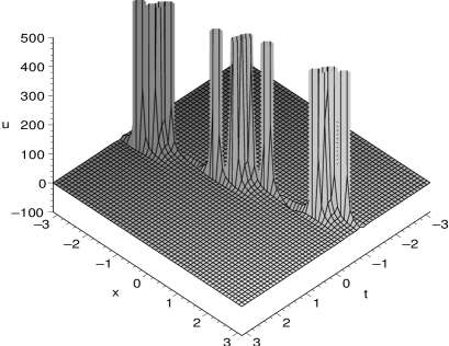
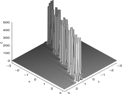
Figure 1: 1-complexiton - $\alpha_{1}=0,\,\beta_{1}=1$ (left)     1-complexiton - $\alpha_{1}=1,\,\beta_{1}=1$ (right)

Complexiton solutions of higher order are complicated but special ones can be presented by taking derivatives of eigenfunctions with respect to the involved parameters [7, 15]. Complexiton solutions are singular and they are not travelling waves. It is clear that the 1-complexiton above is not a travelling wave since $\beta_{1}\neq 0$. Moreover, based on the Painlevé property of the KdV equation, the singularities of complexitons are all poles of second order with respect to $x$. This is obvious for the 1-complexiton above, since $u$ has no pole singularity (the numerator of $u$ will be zero) if the function $\Delta_{1}\sin\xi_{1}+\delta_{1}\sinh\xi_{2}$ is zero and its spatial derivative $2\Delta_{1}\delta_{2}(\cos\xi_{1}+\cosh\xi_{2})$ is also zero, where $\xi_{1}=2\delta_{1}(x-\bar{\beta}_{1}t)+2\kappa_{1}$ and $\xi_{2}=2\Delta_{1}(x+\bar{\alpha}_{1}t)+2\gamma_{1}$.

3 TODA LATTICE EQUATION

Let us second consider the Toda lattice equation

$$\dot{a}_{n}=a_{n}(b_{n-1}-b_{n}),\quad\dot{b}_{n}=a_{n}-a_{n+1},$$ (9)

where $\dot{a}_{n}=\frac{da_{n}}{dt}$ and $\dot{b}_{n}=\frac{db_{n}}{dt}$. Under the transformation

$$a_{n}=1+\frac{d^{2}}{dt^{2}}\log\tau_{n}=\frac{\tau_{n+1}\tau_{n-1}}{\tau_{n}^{2}},\quad b_{n}=\frac{d}{dt}\log\frac{\tau_{n}}{\tau_{n+1}}=\frac{\dot{\tau}_{n}\tau_{n+1}-\tau_{n}\dot{\tau}_{n+1}}{\tau_{n}{\tau}_{n+1}},$$ (10)

the Toda lattice equation (9) becomes

$$\bigl{[}D_{t}^{2}-4\sinh^{2}(\frac{D_{n}}{2})\bigr{]}\tau_{n}\cdot\tau_{n}=0,$$

where $D_{t}$ and $D_{n}$ are Hirota’s operators. That is,

$$\ddot{\tau}_{n}\tau_{n}-(\dot{\tau}_{n})^{2}-\tau_{n+1}\tau_{n-1}+\tau_{n}^{2}=0.$$ (11)

The Casoratian technique [17] is one of the ways to solve the bilinear Toda lattice equation (11). The corresponding solutions to the bilinear Toda lattice equation (11) are determined by the Casorati determinant:

$$\tau_{n}=\textrm{Cas}(\phi_{1},\phi_{2},\cdots,\phi_{N}):=\left|\begin{array}[]{cccc}\phi_{1}(n)&\phi_{1}{(n+1)}&\cdots&\phi_{1}{(n+N-1)}\\ \phi_{2}(n)&\phi_{2}{(n+1)}&\cdots&\phi_{2}{(n+N-1)}\\ \vdots&\vdots&\ddots&\vdots\\ \phi_{N}(n)&\phi_{N}{(n+1)}&\cdots&\phi_{N}{(n+N-1)}\end{array}\right|,$$ (12)

and the Casoratian technique requires [19]

$$\phi_{i}(n+1)+\phi_{i}(n-1)=\displaystyle\sum_{j=1}^{N}\lambda_{ij}\phi_{j}(n),\quad\partial_{t}\phi_{i}(n)=\phi_{i}(n+\delta),\quad 1\leq i\leq N,$$ (13)

where $\delta=\pm 1$ and $\lambda_{ij}$ are arbitrary real constants. Similarly, we only need to consider the Jordan form for the coefficient matrix $\Lambda=(\lambda_{ij})$. Assume that two types of Jordan blocks of the coefficient matrix $\Lambda=(\lambda_{ij})$ are specified as in the case of the KdV equation in the last section. Then, based on the solution structures of eigenfunctions associated with eigenvalues of different types, we can similarly have four Casoratian solution situations:

$\begin{array}[]{ll}\textrm{Rational solutions:}&\textrm{Type 1 with $\lambda_{i}=\pm 2$},\vspace{1mm}\\ \textrm{Negaton solutions:}&\textrm{Type 1 with $\lambda_{i}<-2$}\ \textrm{or}\ \lambda_{i}>2,\vspace{1mm}\\ \textrm{Positon solutions:}&\textrm{Type 1 with $-2<\lambda_{i}<2$},\vspace{1mm}\\ \textrm{Complexiton solutions:}&\textrm{Type 2 with complex eigenvalues.}\end{array}$

Case $k_{i}=1$ of Type 1: We have

$$\phi_{i}(n+1)+\phi_{i}(n-1)=\lambda_{i}\phi_{i}(n),\quad\partial_{t}\phi_{i}(n)=\phi_{i}(n+\delta),$$ (14)

where $\delta=\pm 1$ and $\lambda_{i}=\textrm{consts.}$ Its general eigenfunctions are:

$$\phi_{i}=C_{1i}(\delta n+\varepsilon t)\varepsilon^{n}\textrm{e}^{\varepsilon t}+C_{2i}\varepsilon^{n}\textrm{e}^{\varepsilon t},\quad\lambda_{i}=2\varepsilon,$$

$$\phi_{i}=C_{1i}\textrm{e}^{t\cos k_{i}}\cos({k_{i}n+\delta t\sin k_{i}})+C_{2i}\textrm{e}^{t\cos k_{i}}\sin({k_{i}n+\delta t\sin k_{i}}),\quad\lambda_{i}=2\cos k_{i}$$

$$\phi_{i}=C_{1i}\varepsilon^{n}\textrm{e}^{k_{i}n+\varepsilon t\textrm{e}^{\delta k_{i}}}+C_{2i}\varepsilon^{n}\textrm{e}^{-k_{i}n+\varepsilon t\textrm{e}^{-\delta k_{i}}},\quad\lambda_{i}=2\varepsilon\cosh k_{i},$$

where $\varepsilon=\pm 1$, $|\cos k_{i}|<1$ for the second type of eigenfunctions, $\cosh k_{i}>1$ for the third type of eigenfunctions, and $C_{1i}$ and $C_{2i}$ are arbitrary real constants. These three types of eigenfunctions lead to rational solutions (see, for example, [18]), negatons and positons (see, for example, [2]), respectively.

Case $l_{i}=1$ of Type 2: To construct complexitons, we solve

$$\left\{\begin{array}[]{l}\phi_{1}(n+1)+\phi_{1}(n-1)=\alpha\phi_{1}(n)-\beta\phi_{2}(n),\vspace{2mm}\\ \phi_{2}(n+1)+\phi_{2}(n-1)=\beta\phi_{1}(n)+\alpha\phi_{2}(n),\end{array}\right.\quad\left\{\begin{array}[]{l}\partial_{t}\phi_{1}(n)=\phi_{1}(n+\delta),\vspace{2mm}\\ \partial_{t}\phi_{2}(n)=\phi_{2}(n+\delta),\end{array}\right.$$ (15)

where $\delta=\pm 1$ and $\alpha,\beta=\textrm{consts.}$ Assume that

$$\alpha+\beta\sqrt{-1}\,=\lambda=2\cosh k=\textrm{e}^{k}+\textrm{e}^{-k},\ k=a+b\sqrt{-1}\,,$$

where $a$ and $b$ are real, and then

$$\alpha=2\cosh a\cos b,\ \beta=2\sinh a\sin b.$$

View (15) as a compact equation like (14) where $\lambda=a+b\sqrt{-1}$, and then using the third type of eigenfunctions above, we can generate the corresponding eigenfunctions of (15):

$$\left\{\begin{array}[]{l}\phi_{1}(n)=c\textrm{e}^{na+t\textrm{e}^{\delta a}\cos\delta b}\cos(nb+t\textrm{e}^{\delta a}\sin\delta b)+d\textrm{e}^{-na+t\textrm{e}^{-\delta a}\cos\delta b}\cos(nb+t\textrm{e}^{-\delta a}\sin\delta b),\vspace{2mm}\\ \phi_{2}(n)=c\textrm{e}^{na+\textrm{e}^{\delta a}\cos\delta b}\sin(nb+t\textrm{e}^{\delta a}\sin\delta b)-d\textrm{e}^{-na+t\textrm{e}^{-\delta a}\cos\delta b}\sin(nb+t\textrm{e}^{-\delta a}\sin\delta b).\end{array}\right.$$ (16)

This set of eigenfunctions yields the $\tau$-function of 1-complexiton:

$$\tau_{n} = \textrm{Cas}(\phi_{1}(n),\phi_{2}(n))$$ (17)

$$= 2cd\,\textrm{e}^{2t\cosh\delta a\cos\delta b}\sin(2nb+b+2t\cosh\delta a\sin\delta b)\sinh a$$

$$+c^{2}\textrm{e}^{2na+a+2t\textrm{e}^{\delta a}\cos\delta b}\sin b-d^{2}\textrm{e}^{-2na-a+2t\textrm{e}^{-\delta a}\cos\delta b}\sin b\,,$$

where $\delta=\pm 1$ and $a,b,c,d=\textrm{consts.}$ In particular, $c=\pm d$ leads to the $\tau$-function:

$$\tau_{n} = 2c^{2}\,\textrm{e}^{2t\cosh\delta a\cos\delta b}\sinh(2na+a+2t\sinh\delta a\cos\delta b)\sin b$$

$$\pm 2c^{2}\,\textrm{e}^{2t\cosh\delta a\cos\delta b}\sin(2nb+b+2t\cosh\delta a\sin\delta b)\sinh a\,.$$

The resulting 1-complexiton solution of the Toda lattice equation (9) is given by (10) where $\tau_{n}$ is presented in (17). Two special cases with $\delta=c=d=1$ of this 1-complexiton solution are depicted in Figures 2 and 3.

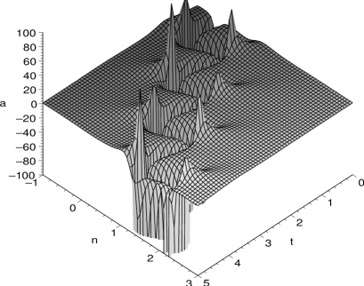
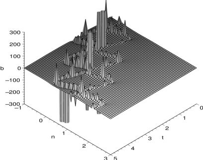
Figure 2: 1-complexiton $a_{n}$ - $2a=b=2$ (left)    1-complexiton $b_{n}$ - $2a=b=2$ (right)

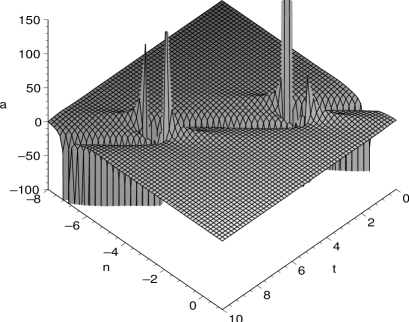
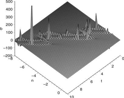
Figure 3: 1-complexiton $a_{n}$ - $a=-b=1$ (left)    1-complexiton $b_{n}$ - $a=-b=1$ (right)

Complexiton solutions of higher order are complicated but special ones can be constructed by computing derivatives of eigenfunctions with respect to the involved parameters [19].

4 CONCLUDING REMARKS

There is a correspondence between the characteristic linear problems of the KdV equation and the Toda lattice equation:

$$\begin{array}[]{rcl}\partial_{x}^{2}&\Leftrightarrow&\phi(n+1)+\phi(n-1)-2\phi(n),\vspace{2mm}\\ -\partial_{x}^{2}\phi=\lambda\phi&\Leftrightarrow&\phi(n+1)+\phi(n-1)=\lambda\phi(n),\vspace{2mm}\\ -\partial_{x}^{2}\phi=\lambda\phi&\Leftrightarrow&-\phi(n+1)-\phi(n-1)+2\phi(n)=(-\lambda+2)\phi(n),\end{array}$$

and a correspondence between the eigenvalues of the characteristic linear problems:

$$\begin{array}[]{lcr}\lambda=0,>0,<0\ \textrm{and $\lambda=$ complex}&\Leftrightarrow&|\lambda|=2,<2,>2\ \textrm{and $\lambda=$ complex},\ \textrm{respectively}.\end{array}$$

We can also observe the correspondence between the KdV equation and its characteristic linear problem $-\partial_{x}^{2}\phi=\lambda\phi$. The characteristic equation of $-\partial_{x}^{2}\phi=\lambda\phi$ is

$$-m^{2}-\lambda=0.$$

Therefore, for example, we see that

$$\begin{array}[]{rcl}\lambda\ \textrm{is positive}&\Leftrightarrow&m\ \textrm{is purely imaginary},\vspace{2mm}\\ \lambda\ \textrm{is complex}&\Leftrightarrow&m\ \textrm{is complex but not purely imaginary}.\end{array}$$

Together with other obvious correspondences, this implies that

$$\begin{array}[]{rcl}\lambda=0&\Leftrightarrow&\textrm{KdV rational solutions},\vspace{2mm}\\ \lambda<0&\Leftrightarrow&\textrm{KdV solitons and negatons},\vspace{2mm}\\ \lambda>0&\Leftrightarrow&\textrm{KdV positons},\vspace{2mm}\\ \lambda=\ \textrm{complex}&\Leftrightarrow&\textrm{KdV complexitons.}\end{array}$$

It then follows that the obtained complexiton solutions to the KdV equation and the Toda lattice equation satisfy the two criteria for complexiton solutions stated in the introduction, indeed. Because of the characteristic in the second criterion, complexitons may play a role similar to the one that the imaginary unit $\sqrt{-1}$ plays in physics.

We also mention that the Wronskian determinants and the Casorati determinants give many other solutions if different types of eigenvalues are allowed. Such solutions are called interaction solutions among determinant solutions of different kinds. For higher dimensional integrable equations, the solution situations are much more diverse [20, 21] and the problem of classifying solutions is extremely difficult [22]. It is hoped that the study of complexitons could further assist in understanding, identifying and classifying nonlinear integrable differential equations and their exact solutions.

References

[1]C. Rasinariu, U. Sukhatme and A. Khare,
J. Phys. A: Math. Gen. 29 (1996) 1803.
[2]K. Maruno, W.X. Ma and M. Oikawa,
J. Phys. Soc. Jpn. 73 (2004) 831.
[3] V.B. Matveev,
Phys. Lett. A 166 (1992) 205.
[4]
A.A. Stahlhofen and V.B. Matveev,
J. Phys. A: Math. Gen. 28 (1995) 1957.