Self–pulsing dynamics of ultrasound in a magnetoacoustic resonator

Abstract

A theoretical model of parametric magnetostrictive generator of ultrasound is considered, taking into account magnetic and magnetoacoustic nonlinearities. The stability and temporal dynamics of the system is analized with standard techniques revealing that, for a given set of parameters, the model presents a homoclinic or saddle–loop bifurcation, which predicts that the ultrasound is emitted in the form of pulses or spikes with arbitralily low frequency.

I Introduction

Magnetostriction is essentally a nonlinear phenomenon, which accounts for the change of dimension of a magnetic material under applied magnetic fields. However, most of the applications of this phenomenon consider small amplitude fields and consequently exploit only their linear properties, as is the case of electromagnetic-acoustic transducers. The consideration of nonlinearities in the description of this process lead to the discovery of new properties, such as the parametric wave phase conjugation (WPC), a phenomena which is actually an active field of research with promising applications into acoustic microscopy Brysev00 or harmonic imaging Krutyansky02 . A review on WPC theory and methods can be found in Brysev98 . There is also increasing interest in the developement of magnetostrictive transducers working at high powers, where nonlinear effects are not negligible. The advances in this field come in paralel with the search of novel magnetic materials with high magnetostriction values.

On the other side, parametric phenomena in different fields of nonlinear science share many common features, such as bistability, self-pulsations and chaos among others. Is precisely this analogy that motivates our search for complex dynamical phenomena in parametrically driven magnetoacoustic systems.

Different models have been proposed for the description of magnetoacoustic interaction in ferromagnetic materials. Also, many experimental progress in this field has been achieved, and the main parameters involved in the process have been determined Brysev200 . In this paper we analize the dynamical behaviour of this system in the presence of magnetic nonlinearity. It is shown that a cubic magnetic nonlinearity is responsible for the appearance of new effects not reported before in this system, such as self-pulsing dynamics and spiking behaviour, related to the existence of homoclinic bifurcations

II The model

The physical system considered in this paper consists in a electric $RLC$ circuit, driven by an external ac source at frequency $2\omega$ and variable amplitude $\varepsilon$. The inductance coil, with density of turns $n$, transverse section $S$ and length $L,$ contains a ferromagnetic ceramic material which acts as an acoustical resonator and is the origin of nonlinearities in the system when the driving $\varepsilon$ is high enough. A theoretical model for this system has been derived in the resonant case in Streltsov97 . We review here the details of the derivation for convenience.

The equation for the circuit is $\varepsilon_{R}+\varepsilon_{C}+\varepsilon_{L}=\varepsilon_{ext}$, where $\varepsilon_{ext}=\mathcal{E}\cos(2\omega t),$ $\varepsilon_{R}=IR,$ $\varepsilon_{C}=q/C$, and $\varepsilon_{L}$ depends nonlinearly on the magnetic fields.

We consider two effects that introduce the nonlinearities in the problem. The first source of nonlinearity results from magnetoacoustic interaction, which appears via phonon-magnon proccesses. In the case of parametric magnetostriction ceramics, the generation of ultrasound takes place at half of the frequency of the driving. This process is represented, in general, by a lagrangian density term in the form $\mathcal{L}_{int}=\alpha_{ijk}H_{i}u_{j}u_{k}$,Streltsov97 where $u_{k}$ is the acoustic displacement component in the direction $k$ ($k=x,y,z$) and $\alpha$ has in general tensor character.

The total magnetic induction $H$ acting along the axis of the material is the result of three contributions: a static field $H_{0}$ produced, e.g. by a permanent magnet surrounding the active ceramic material or a coil carrying a stationary current, an alternating field $H_{q}\left(t\right)$ induced by the ac current in the circuit, and finally a field produced by material deformations $H_{int}$, which results from the magnetoacoustic interaction. From the lagrangian density it follows that, in the case of longitudinal waves propagating in the $z$ axis ($u_{x}=u_{y}=0)$, the acousto-induced magnetic field has the form

$$H_{int}=-\alpha\frac{1}{V}\mathop{\displaystyle\int}u(\mathbf{r},t)^{2}dV,$$ (1)

where $\alpha=\alpha_{zzz}$ is the coefficient of coupling between the active medium of volume $V$ and the pump source. Thus, the effective magnetic induction takes the form

$$H=H_{0}+H_{q}(t)+H_{int}(t).$$ (2)

where we assume that the relation $H_{0}>>H_{q}(t),H_{int}(t)$ holds. Alternatively, $H$ given by (2) can be considered as a nonlinear pumping field Preobrazhensky93 . Note that the appearance of the subharmonic field saturates the magnetic field value, and modifies the effective pumping.

A second source of nonlinearity is typical of ferromagnetic materials. We assume that, for weak saturation, the scalar nonlinear relation between the magnetic field and the magnetic induction, $B=\mu\left(H\right)H$, can be written, following AbdAlla87 , as

$$B=\mu H+\frac{1}{6}\mu_{0}\chi^{(3)}H^{3},$$ (3)

where $\mu$ is linear the permeability of the material and $\chi^{(3)}$ the third order magnetic susceptibility, which in turn depends on the frequency.

Applying the Faraday law under the previous assumptions, considering only resonant terms oscillating at the frequency of the driving $2\omega$, and neglecting terms higher than quadratic in $H_{q}$ and $H_{int}$, we get

$$\varepsilon_{L} = N\frac{d\Phi_{B}}{dt}=N\frac{d}{dt}\mathop{\displaystyle\int}\mathbf{B}~{}d\mathbf{s=}\mathcal{L}\frac{dI}{dt}+$$

$$\mu N\frac{d}{dt}\mathop{\displaystyle\int}H_{int}~{}ds+\mu_{0}\chi^{(3)}N\frac{d}{dt}\mathop{\displaystyle\int}H_{0}H_{q}H_{int}~{}ds,$$

where $I=dq/dt$ is the electrical current in the circuit, $\mathcal{L}$ is the inductance and $H_{q}=NI/L.$ In terms of the charge in the capacitor, and taking into account that $V=SL$ and that $n=N/L$ is the density of turns, the circuit equation takes the form

$$\mathcal{L}\frac{d^{2}q}{dt^{2}}+R\frac{dq}{dt}+\frac{q}{C}=\mathcal{E}\cos(2\omega)+\mu n\alpha\frac{d}{dt}\mathop{\displaystyle\int}u^{2}~{}dV+$$

$$\mu_{0}\chi^{(3)}n^{2}H_{0}\alpha\frac{d}{dt}\left(\frac{dq}{dt}\mathop{\displaystyle\int}u^{2}~{}dV\right),$$ (5)

where the last two terms represent the nonlinearities related magnetoelastic interaction and magnetic nonlinearity respectively.

Let us consider now the evolution of the acoustic wave. Considering the current induced magnetic field $H_{q}$ as the main source term, we find Preobrazhensky93

$$\frac{1}{v^{2}}\frac{\partial^{2}u}{\partial t^{2}}-\nabla^{2}u=\alpha H_{q}(t)u=\alpha n\frac{dq}{dt}u,$$ (6)

where $v$ is the propagation velocity of sound in the material. Here the effect of the acousto-induced magnetic field (quadratic in the small coupling constant $\alpha$) has been neglected. However, we have checked that the consideration of this small term do not imply qualitative changes in the results reported below.

We consider solutions of Eqs. (5) and (6) in the form of quasi-harmonic waves, i.e., whose amplitudes are slowly varying in time. In this case we can write

$$q\left(t\right) =\frac{1}{2}\left[Q\left(t\right)\exp\left(2i\omega t\right)+c.c.\right],$$ (7a)

$$u\left(\mathbf{r},t\right) =\frac{1}{2}\left[U\left(t\right)\exp\left(i\omega t\right)+c.c.\right]g\left(\mathbf{r}_{\bot}\right)\sin\left(kz\right),$$ (7b)

where $$u\left(\mathbf{r},t\right) k=m\pi/L 2\omega=1/\sqrt{\mathcal{L}C}$$ has the form of cavity modes of the acoustical resonator, define the cavity resonances, is the pumping frequency resonant with the circuit, and

$$\left|\frac{dX}{dt}\right|<<\left|\omega X\right|,$$ (8)

with $X=Q$ or $U,$ represents the slowly-varying envelope approximation.

Under these assumptions, the slow amplitudes obey the evolution equations

$$\frac{dQ}{dt} =iE-\gamma_{Q}Q+\xi_{1}U^{2}+i\xi_{2}\left|U\right|^{2}Q,$$ (9a)

$$\frac{dU}{dt} =-\gamma_{U}U+\xi_{3}QU^{\ast},$$ (9b)

where $$E=\mathcal{E}/4\omega\mathcal{L} \gamma_{Q}=R/2\mathcal{L}\ \gamma_{U}$$, and and represent the electric and acoustic losses respectively. The last parameter is introduced phenomenologically, and take into account the losses due mainly to radiation from the boundaries. The coefficients of the nonlinear terms are defined as

$$\xi_{1} =\frac{\mu n\alpha L}{8\mathcal{L}}\mathop{\displaystyle\int}g\left(\mathbf{r}_{\bot}\right)^{2}\text{d}\mathbf{r}_{\bot},$$

$$\xi_{2} =\frac{\omega\mu_{0}\chi^{(3)}n^{2}\alpha H_{0}L}{4\mathcal{L}}\mathop{\displaystyle\int}g\left(\mathbf{r}_{\bot}\right)^{2}\text{d}\mathbf{r}_{\bot},$$ (10)

$$\xi_{3} =\frac{v^{2}n\alpha}{2}.$$

Equations (9) are the model considered in Streltsov97 with some corrections. This system can be further simplified using the normalizations

$$Q=\left(\frac{\gamma_{U}}{\xi_{3}}\right)X,\ \ U=\sqrt{\frac{\gamma_{U}\gamma_{Q}}{\xi_{1}\xi_{3}}}Y,\ \ E=\left(\frac{\gamma_{U}\gamma_{Q}}{\xi_{3}}\right)\mathcal{P},$$ (11)

which leads to the model

$$\frac{dX}{d\tau} =\mathcal{P}-X+Y^{2}+i\eta\left|Y\right|^{2}X,$$ (12)

$$\frac{dY}{d\tau} =-\gamma\left(Y-XY^{\ast}\right),$$

where $\gamma=\gamma_{U}/\gamma_{Q}$ is the ratio between losses, $\tau=\gamma_{Q}t$ is a dimensionless time and

$$\eta=\frac{4\omega H_{0}\gamma_{U}\chi^{(3)}}{\alpha v^{2}\mu_{r}}.$$ (13)

remains as the single parameter of nonlinearity, with $\mu_{r}=\mu/\mu_{0}$. Due to the number of parameters involved in $\eta$, it can be varied over a wide range of values. Note that Eqs. (12) also possess the symmetry $Y\rightarrow-Y$.

III Stationary solutions and stability

Equations (12) possess two kinds of stationary solutions. For small pump values, the acoustic subharmonic field is absent, and the homogeneous trivial solution is readily found as

$$\left|X\right|=\mathcal{P},\ \left|Y\right|=0.$$ (14)

For higher values of the pump, the trivial solution becomes unstable and the acoustic subharmonic field is switched-on. The corresponding values of the amplitudes are given by

$$\left|X\right|=1,\ \ \left|Y\right|^{2}=\frac{1\pm\sqrt{\mathcal{P}^{2}(1+\eta^{2})-\eta^{2}}}{1+\eta^{2}},$$ (15)

and the bifurcation occurs at a critical (threshold) pump given by

$$\mathcal{P}_{th}=1,$$ (16)

which is independent of the value of the nonlinearity coefficient $\eta$.

From (15) it also follows that the acoustic field shows bistability, i.e., both solutions coexist for pump values between $\mathcal{P}_{b}$ and $\mathcal{P}_{th}$, where $\mathcal{P}_{b}$ corresponds to the turning point of the solution and is given by

$$\mathcal{P}_{b}=\sqrt{\frac{\eta^{2}}{1+\eta^{2}}}.$$ (17)

We consider next the stability of the homogeneous solutions (15), by means of the well known linear stability analysis technique. Substituting in Eqs. (12) and their complex conjugate a perturbed solution in the form $x_{i}\left(t\right)=\overline{x}_{i}+\delta x_{i}(t),$ where $\overline{x}_{i}$ is a vector with the particular stationary values, and linearizing the resulting equations around the small perturbations, one obtains that $\delta x_{i}\sim e^{\lambda t}$, where $\lambda$ are the eigenvalues of the stability matrix that relates the vector of the perturbations with their temporal derivatives. The instability of the solution is determined by the existence of positive real parts of the roots $\lambda$ of the fourth-order characteristic polynomial

$$P\left(\lambda\right)=\lambda^{4}+c_{1}\lambda^{3}+c_{2}\lambda^{2}+c_{3}\lambda+c_{4},$$ (18)

where

$$c_{1} =2\left(1+\gamma\right),$$

$$c_{2} =4\gamma+1+\left|Y\right|^{2}\left(\eta^{2}\left|Y\right|^{2}-4\gamma\right),$$

$$c_{3} =2\gamma\left(1-2\left|Y\right|^{2}\left(1+\gamma-\eta^{2}\left|Y\right|^{2}\right)\right),$$

$$c_{4} =4\gamma^{2}\left|Y\right|^{2}\left(-1+\left|Y\right|^{2}\left(1+\eta^{2}\right)\right),$$

with $\left|Y\right|^{2}$ given by Eq. (15). Since we are interested in the existence of dynamical behaviour, we search for a pair of complex conjugate eigenvalues, which denote the occurrence of a Hopf (oscillatory) instability. Following the Hurwitz criterion (see, e.g. Haken83 ), the condition for Hopf instability $\lambda=\pm i\omega$ is given by $c_{3}(c_{1}c_{2}-c_{3})-c_{1}^{2}c_{4}=0,$ or

$$0 =4\eta^{4}\left(\gamma-1\right)\left|Y\right|^{8}+2\eta^{2}\left(\gamma+1\right)^{2}\left|Y\right|^{6}+$$ (19)

$$\eta^{2}\left(4\gamma^{3}-3\gamma-3\right)\left|Y\right|^{4}+$$

$$2\left(\gamma+1\right)^{2}\left(2\gamma+1\right)\left|Y\right|^{2}-\left(2\gamma+1\right)^{2}.$$

The frequency of the oscillations at the bifurcation point, given by the imaginary part of the eigenvalue, is found by substituting $\lambda=i\omega$ in the polynomial. In terms of the acoustic intensity given by the solutions of (19) the frequency reads

$$\omega^{2}=\frac{\gamma}{\gamma+1}\left(1+2\eta^{2}\left|Y\right|^{4}-2\left|Y\right|^{2}\left(\gamma+1\right)\right).$$ (20)

In Fig.1 the domain of existence of Hopf bifurcations (the solutions of Eq. (19)) is represented in the plane $<\eta,\left|Y\right|>,$ for different values of the relative loss parameter $\gamma=0.01,0.1,0.25$ and $0.5.$ The stationary solutions are unstable at the left of each curve, i.e. for small values of $\eta.$ From Fig. 1 also follows that, for a given value of the relative loss parameter $\gamma$, a maximum value of $\eta$ is required for the existence of dynamic solutions.

Figure 1: Domain of existence of oscillatory solutions in the plane $<\eta,|Y|>$, for different loss parameters. Stationary solutions are unstable at the left of each curve.

IV Self–pulsing dynamics near homoclinic bifurcations

In this section the numerical integration of Eqs. (12) is performed in order to demonstrate the existence of dynamical solutions. For typical experimental conditions, $\gamma_{Q}>\gamma_{U}$, and consequently $\gamma<1.$ We take, according to Brysev200 , the value $\gamma=0.1$ for numerical integration, although we note that similar results are obtained for a smaller loss ratio. For this value, the analysis of the previous section (see also Fig. 1, line $c$) shows that the solutions display temporal dynamics when the nonlinearity coefficient take values in the range $0<\eta<0.82.$

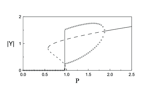
Figure 2: Bifurcation diagram of the ultrasonic field for $\gamma=0.1$ and $\eta=0.7$. Open circles represent maximum and minimum amplitudes of oscillatory solutions.

In Fig. 2 the bifurcation diagram as computed numerically for $\gamma=0.1$ and $\eta=0.7$ is shown. Dashed lines correspond to the analytical solutions given by Eq. (15), and the existence of the backward (inverted) Hopf bifurcation of the upper branch predicted by the theory of the previous section is observed at $\mathcal{P}\approx 1.87$. Dynamical states exist for pump values below this critical point (see also Fig. 1). For higher pump values, the solution is stationary, and the dynamics decay to a fixed point. The upper and lower branches with open circles in Fig. 2 correspond to maximum and minimum values of ultrasonic amplitudes in the oscillating regime. Numerics also show the switch–off of the ultrasonic field when pump is decreased down to a given critical value. This means that, despite bistability, the trivial (zero) solution is a globally attracting solution, which have important consequences on the dynamics of the system.

Similar diagrams are obtained for any value of $\eta$ in the range given above. For small values of the nonlinearity parameter $\eta$, the solutions are quasi-harmonic in time regardless the pump value. However, for larger values of $\eta$ close to limiting value $0.82$ required for the existence of dynamical states, the solutions show a qualitatively different temporal behaviour, not predicted by the linear stability analysis which in fact is valid only near the bifurcation point. Next we report the numerical results for the particular value $\eta=0.7$ corresponding to Fig. 2.

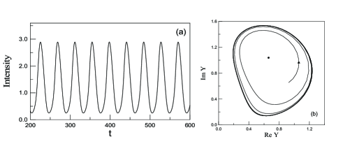
Figure 3: (a) Time dependence of the intensity of the ultrasonic field for $\mathcal{P}=1.35$. The rest of parameters as in Fig. 2. (b) The corresponding phase portrait.

In Fig. 3(a) the amplitude of the ultrasonic field is plotted as a funcion of time for a pump value of $\mathcal{P}=1.35$ far from the bifurcation point at $\mathcal{P}_{th}=1$. The corresponding phase portrait is shown in Fig. 3(b), where the existence of a stable limit cycle is observed. However, when decresing the pump, the ultrasonic field is emmited in the form of periodic pulses or spikes, whose temporal separation (period) depends on the value of the pump amplitude, and increases with it. Close to the emission threshold the time between pulses (interspike period) tends to infinity. An example of the temporal profile of the field amplitude in the spiking regime, and the corresponding phase portraits for the pump value $\mathcal{P}=0.95$ is shown in Fig. 4(a) and (b) respectively.

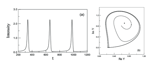
Figure 4: (a) Time dependence of the intensity of the ultrasonic field for $\mathcal{P}=0.95$. The rest of parameters as in Fig. 2. (b) The corresponding phase portrait. The homoclinic point is represented by the open circle.

This behavior denotes the existence of a global bifuraction of the solutions for the parameters considered. As the pump approaches the critical value $\mathcal{P}_{c}=0.904$, the amplitude of the lower branch of the oscillating solutions (open circles in Fig. 2) approaches the lower branch of the stationary solutions (short-dashed line in Fig. 2), which as follows from the linear stability analysis corresponds to a saddle point. The limit cycle at this point connects with the saddle point, and denegerates in a saddle-loop or homoclinic bifurcation. For pump values below $\mathcal{P}_{c}$ the trayectory decays to a fixed point corresponding to the trivial solution.

The period of the limit cycle near a saddle-loop bifurcation is governed by a characteristic scaling law. Linearization of the dynamics around the saddle leads to the following expression for the period Gaspard90

$$T\propto-\frac{1}{\lambda}\ln(\mathcal{P}_{c}-\mathcal{P})$$

where $\mathcal{P}_{c}-\mathcal{P}$ measures the distance to the homoclinic bifurcation (which is assumed small) and $\lambda$ is the eigenvalue in the unstable direction of the saddle point.

Figure 5 shows the numerically evaluated period of the self-pulsed solutions in the whole range where dynamical states exists. Note the divergence in the period at $\mathcal{P}_{c}=0.904.$ In order to check the homoclinic character of the bifurcation, the inset shows the linear fit of the period against $\ln(\mathcal{P}_{c}-\mathcal{P})$ for pump values close to $\mathcal{P}_{c}.$ The slope of the linear fit is found to be $51.4$, in good agreement with the linear stability result $1/\lambda=54.2,$ demonstrating the existence of the saddle-loop bifurcation.

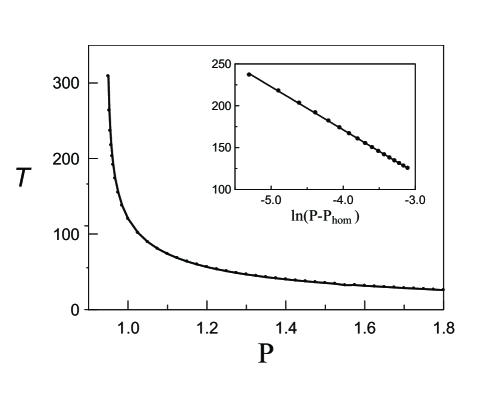
Figure 5: Period of the oscillations as a function of the pump. The insert shows the linear fit.

Finally, when decreasing the pump below the saddle–loop bifurcation point, the subharmonic field is switched-off. Trivial solution acts then as a globally attracting point.

V Conclusion

A model of parametric generation of ultrasound in a ferromagnetic material has been considered, and its stability analyzed, revealing the existence of a Hopf bifurcation leading to self–pulsing dynamics. For selected values of the decay rates and the nonlinearity parameter, the system also show a saddle–loop bifurcation which results in a spiking regime in the emitted ultrasound, where the frequency can take arbitrary low frequencies or firing rates. It has been demonstrated Izhikevich00 that dynamical systems where saddle–loop bifurcations and stable fixed points coexist have also a property called excitability, characterized by Murray (a) perturbations of the rest state beyond a certain threshold induce a large response before coming back to the rest state, and (b) there exist a refractory time during which no further excitation is possible. This properties, which are characteristic in several biological problems (e.g. the behaviour of action potentials in neurons Hodking52 ) and some laser models Krauskopf03 , are being investigated in the context of the acoustical system proposed in this paper.

References

- (1) A. Brysev, L. Krutyansky, P. Pernod and V. Preobrazhensky, Appl. Phys. Lett. 76, 3133-3135 (2000).
- (2) L. Krutyansky, P. Pernod, A. Brysev, F. Bunkin and V. Preobrazhenshy, IEEE Trans. Ultrason., Ferroelect., Freq. Contr. 49, 409-414 (2002).
- (3) A. Brysev, L. Krutyansky and V. Preobrazhensky, Phys. Uspekhi 41, 793–805 (1998).
- (4) A. Brysev, P. Pernod and V. Preobrazhensky, Ultrasonics 38, 834-837 (2000).
- (5) V.N. Streltsov, BRAS Physics Supplement 61, 228-230 (1997).
- (6) V. Preobrazhensky, Jpn. J. App. Phys. 32, 2247-2251 (1993).
- (7) A. Abd-Alla and G. Maugin, J. Acoust. Soc. Am. 82, 1746-1752 (1987).
- (8) H. Haken, Synergetics, Springer-Verlag, Berlin (1983)
- (9) P. Gaspard, J. Chem. Phys. 94, 1 (1990)
- (10) E.M. Izhikevich, Int. J. Bif. Chaos 10, 1171 (2000)
- (11) J.D. Murray, Mathematical biology. Springer (1990)
- (12) A.L. Hodking and A.F. Huxley, J. Physiol. 17, 500 (1952).
- (13) B. Krauskopf, K. Schneider, J. Sieber, S. Wieczorek and M. Wolfrum, Opt. Commum. 215, 367-379 (2003)