Controlling soliton explosions

Abstract

We investigate the dynamics of solitons in generalized Klein-Gordon equations in the presence of nonlinear damping and spatiotemporal perturbations. We will present different mechanisms for soliton explosions. We show (both analytically and numerically) that some space-dependent perturbations or nonlinear damping can make the soliton internal mode unstable leading to soliton explosion. We will show that, in some cases, while some conditions are satisfied, the soliton explodes becoming a permanent, extremely complex, spatiotemporal dynamics. We believe these mechanisms can explain some of the phenomena that recently have been reported to occur in excitable media. We present a method for controlling soliton explosions.

, and

Solitons are used in many important technological applications. Among these applications we can mention long distance communication systems and soliton oscillators in superconducting devices [1].

However, under certain conditions, solitons can become unstable [2, 3, 4]. Such instabilities have been called both soliton breakup and soliton explosions. For instance, Milchev and coworkers have studied the Frenkel-Kontorova model with anharmonic interatomic interactions [2]. They have found that, in the Frenkel-Kontorova model with nonconvex interactions between closest neighbors, a breakup of the kink takes place when the effective amplitude of the sinusoidal substrate potential exceeds a certain critical value.

An extensive discussion of soliton dynamics in the framework of the Frenkel-Kontorova model can be found in the recent book [5].

On the other hand, in Refs. [3] it was predicted that the soliton internal mode can become unstable leading to soliton explosions.

Such instabilities as soliton explosions can affect all the mentioned applications. So it is very important to understand all the possible mechanisms of soliton explosions in order to avoid them.

In the present letter we investigate generalized Klein-Gordon equations as the following

$$\phi_{tt}+R\left(\phi_{t}\right)-\phi_{xx}-G\left(\phi\right)=F(x,t),$$ (1)

where $G\left(\phi\right)=-\partial U\left(\phi\right)/\partial\phi,$ $U\left(\phi\right)$ is a potential function with at least two minima $\phi_{1},\phi_{3}$ and a maximum $\phi_{2}$, such that $U\left(\phi_{1}\right)=U\left(\phi_{3}\right)=0$ , $R\left(\phi_{t}\right)$ are dissipative terms, and $F(x,t)$ represents external perturbations. We are interested in kinks, that is, topological solitons between the points $\phi_{1}$ and $\phi_{3}$. The famous sine-Gordon and $\phi^{4}$-systems are particular cases of Eq. (1).

The topological solitons studied in the present letter possess important applications in condensed matter physics – they describe domain walls in ferromagnets and ferroelectric materials, dislocations in crystals, charge-density waves, interphase boundaries in metal alloys, fluxons in long Josephson junctions and Josephson transmission lines, etc. [6].

We will present different mechanisms for soliton explosions. We will show that in some cases, while some conditions hold, the soliton explosion is permanent.

A soliton destruction is observed when inhomogeneous space-dependent perturbations are present:

$$\phi_{tt}+\gamma\phi_{t}-\phi_{xx}-G\left(\phi\right)=F\left(x\right).$$ (2)

We should say that the zeroes of $F\left(x\right)$ are candidates for equilibrium positions for the soliton [3]. If $F\left(x\right)$ possesses only one zero $x_{0}^{\ast}$ ($F\left(x_{0}^{\ast}\right)=0$), then it is a stable position for the soliton if $\left(\partial F/\partial x\right)_{x_{0}^{\ast}}>0$. Otherwise, the position is an unstable equilibrium. The opposite is true for the antisoliton. The center of mass of a soliton can make oscillations around a stable zero of $F\left(x\right)$, and it can move away from an unstable one. However, when $F\left(x\right)$ has an unstable zero at $x=x_{0}^{\ast}$ and additionally, the following conditions holds $\lim_{x\rightarrow\pm\infty}F\left(x\right)=\mp F_{\infty}$, $F_{\infty}>0$ and $F_{\infty}$ is larger than some critical value, then the soliton can be destroyed and an antisoliton is “created” in the equilibrium position $x=x_{0}^{\ast}$.

When the soliton is in an unstable equilibrium position, it is “stretched” by the pair of forces that are acting on its body in opposite directions. And there is a limit for the magnitude of the pair of forces that the soliton can resist. Nevertheless, there is a more subtle mechanism for soliton destruction. When a soliton is close to an unstable equilibrium position, many internal shape modes of the soliton can be excited [7, 3]. If $\left(\partial^{2}F/\partial x^{2}\right)_{x_{0}^{\ast}}$ is larger than some critical value, then the first internal shape mode can become unstable and this instability can lead to the soliton destruction. In this phenomenon the soliton decays into an antisoliton and two solitons. What is interesting in this situation is that $F\left(x\right)$ can be a localized perturbation.

Suppose we are interested in the stability of a soliton situated in equilibrium positions created by the inhomogeneous force $F\left(x\right)$. Using an inverse-problem method [3, 8] we construct an exact solution $\phi_{k}\left(x\right)$ with the topological properties of a kink-soliton. Then we investigate the stability of the solution solving the spectral problem

$$\widehat{L}f\left(x\right)=\Gamma f\left(x\right),$$ (3)

where $\widehat{L}=-\partial_{xx}-\left[\partial G\left(\phi\right)/\partial\phi\right]_{\phi=\phi_{k}}$, $\Gamma=-\left(\lambda^{2}+\gamma\lambda\right)$.

Let us discuss some examples in detail.

The force

$$F\left(x\right)=\alpha\tanh\left(\beta x\right)\left[\delta+\varepsilon\operatorname{sech}^{2}\left(\beta x\right)\right],$$ (4)

can sustain a kink-soliton equilibrated at point $x=0$.

When we solve the stability problem (3) we obtain the following eigenvalues of the discrete spectrum (for simplicity we assume $\delta=\left(\alpha^{2}-1\right)/2$, $\varepsilon=\left(4\beta^{2}-\alpha^{2}\right)/2$ and $G\left(\phi\right)=\left(\phi-\phi^{3}\right)/2$: $\Gamma_{n}=\beta^{2}\left(\Lambda+2\Lambda n-n^{2}\right)-\frac{1}{2}$, where $\Lambda\left(\Lambda+1\right)=3\alpha^{2}/2\beta^{2}$, $n<\Lambda$.

The translational mode of the soliton is stable if $2\beta^{2}\Lambda>1$. If this condition is not satisfied, this just means that the soliton center of mass will move away from the unstable equilibrium position $x=0$. This does not necessarily lead to the soliton destruction.

However, if the following condition holds:

$$2\beta^{2}\left(3\Lambda-1\right)<1,$$ (5)

the soliton first shape mode is unstable. In this case, the soliton can be destroyed!

In the very special (but also very illustrative) case $\varepsilon=0$, we have that for $4\beta^{2}>1$, the translational mode is stable. This means the equilibrium position $x=0$ is stable for the soliton. The soliton center of mass can perform oscillations around point $x=0$. If $4\beta^{2}<1$ (but $10\beta^{2}>1$), the translational mode is unstable. In this case, the soliton can move away from point $x=0$, but it conserves its very characteristic shape because the internal modes are still stable. However, if $10\beta^{2}<1$, then the first internal (shape) mode becomes unstable. In this situation the soliton can explode. If we apply a spatiotemporal perturbation that periodically (in time) creates this instability in the place where the soliton is situated  at that instant, then the result will be a highly nonstationary spatiotemporal state where the soliton is not allowed to recover its original shape. The soliton is in a permanent explosion.

Another very important example of equation (1) is the sine-Gordon equation (i.e. $G(\phi)=-\sin\phi$). Suppose $F(x)=2\left(\beta^{2}-1\right)\sinh\left(\beta x\right)\cosh^{-2}\left(\beta x\right)$. This perturbation creates an equilibrium position for the sine-Gordon soliton at point $x=0$. When we solve the eigenvalue problem (3) for the sine-Gordon soliton in the presence of this external force we get the following discrete spectrum: $\Gamma_{n}=\beta^{2}\left(\Lambda+2\Lambda n-n^{2}\right)-1$, where $\Lambda\left(\Lambda+1\right)=2/\beta^{2}$. The integer part of $\Lambda$ yields the number of eigenvalues in the discrete spectrum. For $\beta^{2}>1$, the translational mode is stable and there are no internal modes. If $\left(1/3\right)<\beta^{2}<1$, then the translational mode is unstable (but still there are no internal modes). When $\left(1/6\right)<\beta^{2}<\left(1/3\right)$ there appears an internal shape mode, which is stable. For $\beta^{2}<2/\left[\Lambda_{\ast}\left(\Lambda_{\ast}+1\right)\right]$, where $\Lambda_{\ast}=\left(5+\sqrt{17}\right)/2$, the first internal shape mode becomes unstable. This perturbation can destroy the sine-Gordon soliton.

We should say that a soliton, moving in a medium that is homogeneous everywhere except for a zone where the conditions for the instabilities hold, can undergo dramatic transient changes. But when the soliton leaves the mentioned zone, it will return to its original steady state shape.

How can we produce a permanent soliton explosion? We can use time-dependent perturbations:

$$\phi_{tt}+\gamma\phi_{t}-\phi_{xx}-G\left(\phi\right)=F_{1}\left(x\right)+F_{2}\left(x,t\right),$$ (6)

where $F_{1}\left(x\right)$ is a perturbation that creates a potential well for the soliton (i.e. $F\left(x\right)$ possesses a zero $x_{0}^{\ast}$ such that $\left(\partial F/\partial x\right)_{x_{0}^{\ast}}>0$) and $F_{2}\left(x,t\right)$ is a space-time perturbation that periodically generates the instabilities conditions. Figure 1 shows an example of those highly complex spatiotemporal behaviors. In all the figures $G\left(\phi\right)=\left(\phi-\phi^{3}\right)/2$. However, similar results are obtained with the sine-Gordon and other Generalized Klein-Gordon equations.

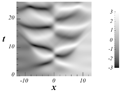
Figure 1: Initial steps of a permanent soliton explosion sustained by a spatiotemporal perturbation as in Eq. (6). Here $F_{1}\left(x\right)=(1/2)A\left(A^{2}-1\right)\tanh\left(Bx\right)$, $F_{2}\left(x,t\right)=(1/2)f_{0}A\left(4B^{2}-A^{2}\right)\cos\left(\omega t\right)\sinh\left(Bx\right)\cosh^{-3}\left(Bx\right)$, $A=1.5$, $B=0.2$, $\gamma=0.1$, $\omega=1$, $f_{0}=3$.

Can we produce permanent soliton explosions without time-dependent external perturbations?

Here we would like to remark that solitons can move with constant velocity (without attenuation) in active and excitable media, and in systems with nonlinear damping even without explicit external forces.

Let us discuss here briefly the importance of nonlinear damping. Linear dissipative systems like the damped harmonic oscillator $\phi_{tt}+\gamma\phi_{t}+\omega_{0}^{2}\phi=0$ cannot sustain oscillations. However, the nonlinear oscillator $\phi_{tt}-b\phi_{t}+a\phi_{t}^{3}+\omega_{0}^{2}\phi=0$ supports a stable limit cycle [9]. The transition from a stable focus to an unstable focus and a stable limit cycle is the result of a Hopf bifurcation. This system is very easy to realize in practice using negative-resistance electronic elements [10].

Soliton systems as the following:

$$\phi_{tt}+R\left(\phi_{t}\right)-\phi_{xx}-G\left(\phi\right)=0,$$ (7)

where $dR\left(\phi_{t}\right)/d\phi_{t}$ is negative for small values of $\left|\phi_{t}\right|$ and positive elsewhere, can support solitons moving with a constant velocity. An example of this kind of systems can be realized in practice using a Josephson junction transmission line where the resistor is a negative-resistance twin-tunnel-diode circuit or a twin-transistor system [10]. In this case, $R\left(\phi_{t}\right)=-b\phi_{t}+a\phi_{t}^{3}$ is a good model.

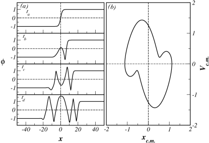
Figure 2: (a) Soliton explosion due to nonlinear damping. Here in Eq. (7): $R\left(\phi_{t}\right)=-b\phi_{t}+a\phi_{t}^{3}$, $a=1$, $b=0.7$. (b) Limit cycle produced with the dynamics of the soliton center of mass in Eq. (8). Here $\Gamma\left(x\right)=1-l/\cosh\left(Dx\right)$, $F\left(x\right)=A\tanh\left(Bx\right)$, $A=0.45$, $B=0.65$, $l=2$, $D=0.65$.

We have investigated the shape mode stability of the soliton in the presence of nonlinear damping as we did before using the spectral problem (3).

Suppose $R\left(\phi_{t}\right)$ possesses two local extrema: a maximum and a minimum such that the value of $\left|R\left(\phi_{t}\right)\right|$ at these extrema is $R_{m}$. If this value is comparable with the absolute value of the extrema of $G\left(\phi\right)$ (let us call it $G_{m}$), then the soliton can be destroyed. In fact, if $R_{m}>G_{m}$ the internal shape mode of the soliton can be unstable and the soliton becomes a highly nonstationary state.

When $F\left(x\right)$ in Eq. (2) has a stable zero, say $x=x_{0}^{\ast}$, the center of mass of a soliton can perform damped oscillations around $x_{0}^{\ast}$. If we wish to sustain these oscillations without explicit time-periodic external forces, then we should resort again to negative damping. Another way to experiment negative damping is when the damping coefficient in Eq. (2) is a function of $x$:

$$\phi_{tt}+\Gamma\left(x\right)\phi_{t}-\phi_{xx}-G\left(\phi\right)=F\left(x\right).$$ (8)

Here $\Gamma\left(x\right)$ is negative in a neighborhood of $x_{0}^{\ast}$ and positive elsewhere. This can be done in a chain of nonlinear oscillators using negative-resistance circuits [10] only in some small interval of the chain. An example of $\Gamma\left(x\right)$ with the required features is $\Gamma\left(x\right)=\gamma\left[1-L/\cosh^{2}\left(Dx\right)\right]$, where $\left(1-L\right)<0$.

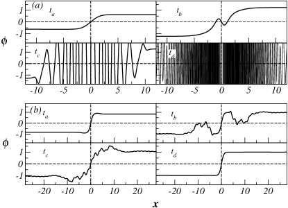
Figure 3: (a) Highly nonstationary spatiotemporal dynamics produced by Eq. (8). Here the simulated equation is the same as in Fig. 2 (b) with $l=6$. (b) The soliton dynamics can be controlled in order to avoid the soliton explosion. Here in Eq. (9) $\gamma=0.1$, $F_{p}\left(x,t\right)=-0.385\tanh\left(Bx\right)\cos\left(\omega t\right)$, $F_{c}\left(x,t\right)=-0.75\tanh\left(Bx\right)\cosh^{-2}\left(Bx\right)$, $B=1$, $\omega=0.2$.

Figure 2 (b) shows a limit cycle which is the result of the dynamics of the soliton center of mass in Eq. (8). However if we are not careful, the soliton can explode also in this system. We have solved the soliton stability problem for this equation. The most important result is that the first internal shape mode is unstable for $L>5/2$. This behavior can be observed in Fig. 3 (a).

Can we control all these types of explosive dynamics? Well, if we can change the parameters of the system, then we can use parameter values that do not lead to soliton explosions. However, sometimes we can not change the parameters. We just are allowed to apply some external perturbation.

Let us pose the following problem:

$$\phi_{tt}+\gamma\phi_{t}-\phi_{xx}-G\left(\phi\right)=F_{p}\left(x,t\right)+F_{c}\left(x\right).$$ (9)

Equation (9) represents a system with explosive behavior as that shown in figures 1, 2 (a) and 3 (a), when the control perturbation $F_{c}\left(x\right)=0$. The problem is to find a controlling perturbation $F_{c}\left(x\right)$. Suppose $F_{p}\left(x,t\right)$ is a function that periodically generates the instability conditions discussed in the first part of the paper. An example can be the following $F_{p}\left(x,t\right)=a\cos\left(\omega t\right)\tanh\left(Bx\right)$. The strategy could be to find a perturbation $F_{c}\left(x\right)$ such that the superposition $F_{p}\left(x,t\right)+F_{c}\left(x\right)$ does not satisfy the instability condition anymore for any $t$.

It is remarkable that this can be achieved using a localized perturbation. For instance $F_{p}\left(x,t\right)=-0.385\cos\left(\omega t\right)\tanh\left(Bx\right)$ is a turbulent-producing perturbation, and $F_{c}\left(x\right)=0.75\sinh\left(Bx\right)\cosh^{-3}\left(Bx\right)$ can control this behavior. This can be seen in Fig. 3 (b).

Similarly, the turbulence created by nonlinear damping can be controlled with a stabilizing perturbation: $\phi_{tt}-\phi_{xx}-b\phi_{t}+a\phi_{t}^{3}-G\left(\phi\right)=F_{c}\left(x\right)$ .

The explanation for these phenomena is based on our analytical results presented above. The perturbation $F_{p}\left(x,t\right)=-0.385\cos\left(\omega t\right)\tanh\left(Bx\right)$ is able to destroy the soliton and produce a highly nonstationary state because the perturbation $F(x)=-0.385\tanh\left(Bx\right)$ leads to the instability of the soliton shape mode (according to our condition (5)). So $F_{p}\left(x,t\right)$ will produce this condition regularly. The soliton will be exposed to this instability again and again. The soliton destruction produces several new solitons and antisolitons which also can be later destroyed because the perturbation makes them unstable too. The control perturbation $F_{c}\left(x\right)$ is able to stabilize the soliton because the total perturbation $F\left(x,t\right)=-0.385\cos\left(\omega t\right)\tanh\left(Bx\right)+0.75\sinh\left(\beta x\right)\cosh^{-3}\left(\beta x\right)$ does not satisfy the shape mode instability condition for any $t$. That is, when we solve the stability problem (3) for $F(x)=-0.385\mu\tanh\left(Bx\right)+0.75\sinh\left(\beta x\right)\cosh^{-3}\left(\beta x\right)$, the internal shape modes are always stable for $-1\leq\mu\leq 1$.

The kink-solitons are examples of a very general phenomenon called topological defects. This set of phenomena includes: topological solitons, vortices and spirals [11]. Although these objects can possess different origin and nature in different physical systems, they all possess very similar dynamical properties [11].

The breakup of topological defects has been observed in experiments in many systems [12].

In different experiments, it has been observed that one topological defect can breakup into several topological defects. In particular, the “elementary” breakup that we have found, where one topological defect breaks up into three topological defects: one antidefect and two defects, has been observed in cardiac tissue [13].

All the situations discussed in the present paper that lead to very complex spatiotemporal behaviors start with soliton breakups (see figures 1, 2 (a), and 3).

At least, the following two different breakup scenarios are documented in experiments [14, 15, 16]. In one case, the breakup (leading to turbulence) occurs when a spatiotemporal external forcing is added to the system [14]. In a second case, the topological defects break after a Hopf bifurcation [16].

We believe that the results of the present paper show that very similar phenomena can occur with kink-solitons in Klein-Gordon systems. We have been able to produce defect-mediated turbulence using spatiotemporal external forcing, and after a Hopf bifurcation generated by nonlinear damping.

A. Bellorín would like to thank OPSU-CNU for support.

References

- [1] A. Hasegawa and Y. Kodama, “Solitons in Optical Communications” (Oxford University Press, New York, 1995); N. Grønbech-Jensen and J. A. Blackburn, Phys.Rev. Lett. 70, 1251 (1993), and references therein.
- [2] A. Milchev, Phys. Rev. B 33, 2062 (1986); A. Milchev and G. M. Mazzucchelli, Phys. Rev. B 38, 2808 (1988); B. A. Malomed and A. Milchev, Phys. Rev. B 41, 4240 (1990); A. Milchev, Phys. Rev. B 42, 6727 (1990); A. Milchev, Physica D 41, 262 (1990); A. Milchev, Th. Fraggis, and St. Pnevmatikos, Phys. Rev. B 45, 10348 (1992).
- [3] J. A. González and J. A. Hołyst, Phys. Rev. B 45, 10338 (1992); J. A. González, L. E. Guerrero, and A. Bellorín, Phys. Rev. E 54, 1265 (1996); J. A. González and B. A. Mello B. A., Phys. Lett. A 219, 226 (1996); J. A. González, B. A. Mello, L. I. Reyes, and L. E. Guerrero, Phys. Rev. Lett. 80, 1361 (1998); J. A. González, A. Bellorín, and L. E. Guerrero, Phys. Rev. E 65, 065601(R) (2002).
- [4] S. T. Cundiff, J. M. Soto-Crespo, and N. Akhmediev, Phys.Rev. Lett. 88, 073903 (2002).
- [5] O. Braun and Y. S. Kivshar, “The Frenkel-Kontorova model” ((Springer-Verlag, Berlin, 2004).
- [6] Y. S. Kivshar and B. A. Malomed, Rev. Mod. Phys. 61, 763 (1989); A. R. Bishop, J. A. Krumhansl, and S. E. Trullinger, Physica D 1, 1 (1980).
- [7] J. A. González and J. A. Hołyst, Phys. Rev. B 35, 3643 (1987).
- [8] J. A. González and F. A. Oliveira, Phys. Rev. B 59, 6100 (1999).
- [9] A. A. Andronov, E. A. Vitt, and S. E. Khaiken, “Theory of Oscillators” (Pergamon, Oxford, 1966); J. Guckenheimer and P. L. Holmes, “Nonlinear Oscillators, Dynamical Systems and Bifurcations of Vector Fields” (Springer-Verlag, Berlin, 1986).
- [10] L. O. Chua, C. A. Desoer, and E. S. Kuh, “Linear and Nonlinear Circuits” (McGraw-Hill, New York, 1987).
- [11] M. C. Cross and P. C. Hohenberg, Rev. Mod. Phys. 65, 851 (1993); I. S. Aranson and L. Kramer, Rev. Mod. Phys. 74, 99 (2002); B. A. Mello, J. A. González, L. E. Guerrero, and E. López-Atencio, Phys. Lett. A 244, 277 (1998).
- [12] M. Courtemanche, L. Glass, and J. P. Keener, Phys. Rev. Lett. 70, 2182 (1993); A. Karma, Phys. Rev. Lett. 71, 1103 (1993); M. Bär and M. Or-Guil, Phys. Rev. Lett. 82, 1160 (1999); Q. Ouyang and J. M. Fleselles, Nature 379, 143 (1996); S. M. Tobias and E. Knobloch, Phys. Rev. Lett. 80, 4811 (1998).
- [13] A. Panfilov and A. Holden, Phys. Lett. A 147, 463 (1990); A. Panfilov and A. Holden, Int. J. Bifurcations and Chaos 1, 119 (1991).
- [14] A. Belmonte, J.-M. Flesselles, and Q. Ouyang, Europhys. Lett. 35, 665 (1996).
- [15] Q. Ouyang, H. L. Swinney, and G. Li, Phys. Rev. Lett. 84, 1047 (2000).
- [16] D. Barkley, Phys. Rev. Lett. 68, 2090 (1992).