Critical bending point in the Lyapunov localization spectra of many-particle systems

Abstract

The localization spectra of Lyapunov vectors in many-particle systems at low density exhibit a characteristic bending behavior. It is shown that this behavior is due to a restriction on the maximum number of the most localized Lyapunov vectors determined by the system configuration and mutual orthogonality. For a quasi-one-dimensional system this leads to a predicted bending point at $n_{c}\approx 0.432N$ for an $N$ particle system. Numerical evidence is presented that confirms this predicted bending point as a function of the number of particles $N$.

The Lyapunov spectrum is an indicator of dynamical instability in the phase space of many-particle systems. It is introduced as the sorted set $\{\lambda^{(n)}\}_{n}$, $\lambda^{(1)}\geq\lambda^{(2)}\geq\cdots$ of Lyapunov exponents $\lambda^{(n)}$, which give the exponential rates of expansion or contraction of the distance between nearby trajectories (Lyapunov vector) and is defined for each independent component of the phase space. In Hamiltonian systems and some thermostated systems, a symmetric structure of the Lyapunov spectra, the so called the conjugate pairing rule, is observed Dre88 ; Eva90 ; Det96a ; Tan02a . One of the most significant points of the Lyapunov spectrum is that each Lyapunov exponent indicates a time scale given by the inverse of the Lyapunov exponent so we can consider the Lyapunov spectrum as a spectrum of time-scales. The smallest positive Lyapunov exponent region of the spectrum is dominated by macroscopic time and length scale behavior, and here some delocalized mode-like structures (the Lyapunov modes) have been observed in the Lyapunov vectors Pos00 ; Eck00 ; Tan02c ; Tan03a ; Mar04 ; Wij03 ; Yan04 ; Tan04a ; For04 ; Tan04b . On the other hand, the largest Lyapunov exponent region of Lyapunov spectrum is dominated by short time scale behavior, and in this region the Lyapunov vectors are localized (Lyapunov localization). The position of the localized region of Lyapunov vectors moves as a function of time. A variety of many-particle systems show Lyapunov localization, for example, the Kuramoto-Sivashinsky model Man85 , a random matrix model Liv89 , map systems Kan86 ; Fal91 ; Gia91 ; Pik98 , coupled nonlinear oscillators Pik01 , and many-disk systems Mil02 ; Tan03b .

Recently, a quantity to measure strength of Lyapunov localization was proposed Tan03b . For each Lyapunov exponent we construct the normalized Lyapunov vector component amplitude $\gamma_{j}^{(n)}\equiv|\delta\mbox{\boldmath$\bf\Gamma$}_{j}^{(n)}|/|\delta\mbox{\boldmath$\bf\Gamma$}^{(n)}|$ for each particle $j$. Here $\delta\mbox{\boldmath$\bf\Gamma$}^{(n)}\equiv(\delta\mbox{\boldmath$\bf\Gamma$}_{1}^{(n)},\delta\mbox{\boldmath$\bf\Gamma$}_{2}^{(n)},\cdots,\delta\mbox{\boldmath$\bf\Gamma$}_{N}^{(n)})$ is the Lyapunov vector for the $n$-th Lyapunov exponent $\lambda^{(n)}$, and $\delta\mbox{\boldmath$\bf\Gamma$}_{j}^{(n)}$ is the contribution of the $j$-th particle to the $n$-th Lyapunov vector. The localization of the $n$-th Lyapunov vector is then

$$\mathcal{W}^{(n)}\equiv\exp\left[-\sum_{j=1}^{N}\left\langle\gamma_{j}^{(n)}\ln\gamma_{j}^{(n)}\right\rangle\right].$$ (1)

The bracket $\langle\cdots\rangle$ in Eq. (1) indicates the time-average. The quantity $-\sum_{j=1}^{N}\langle\gamma_{j}^{(n)}\ln\gamma_{j}^{(n)}\rangle$ in the definition (1) of $\mathcal{W}^{(n)}$ can be regarded as an entropy-like quantity, as $\gamma_{j}^{(n)}$ is a distribution function over the particle index $j$. The quantity $\mathcal{W}^{(n)}$ satisfies the inequality $1\leq\mathcal{W}^{(n)}\leq N$, and can be interpreted as the effective number of particles contributing to the non-zero components of the Lyapunov vector. In a Hamiltonian system it satisfies the conjugate relation $\mathcal{W}^{(\mathcal{D}-j+1)}=\mathcal{W}^{(j)}$ for any $j$ with the phase space dimension $\mathcal{D}$, because of the symplectic structure.

The set of quantities $\{\mathcal{W}^{(n)}\}_{n}$ which we call the Lyapunov localization spectrum, has been calculated previously in many-particle systems with hard-core interactions Tan03b and with soft-core interactions For04 . In these systems, the value of $\mathcal{W}^{(n)}$ usually increases with the Lyapunov index $n$, and this implies that Lyapunov vectors for the largest exponent region are the most localized. The quantity $\mathcal{W}^{(n)}$ has a minimum value of 2, as a minimum of two particles are involved in each collision, and it has been shown numerically that the value of $\mathcal{W}^{(n)}$ for the largest Lyapunov exponent approaches 2 as the density approaches zero Tan03b . It was also shown that $\mathcal{W}^{(n)}$ can detect not only the localized behavior of Lyapunov vectors, but also the de-localized behavior observed in the Lyapunov modes Tan03b .

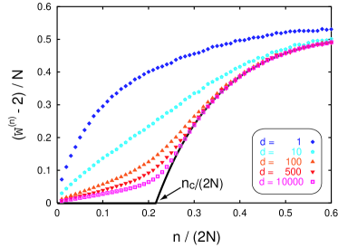
Figure 1: (Color online) The normalized Lyapunov localization spectra $\{(\mathcal{W}^{(n)}-2)/N\}_{n}$ as functions of the normalized Lyapunov index $n/(2N)$ for quasi-one-dimensional $50$ hard-disk systems at different densities given by $d=1$ (diamonds), $d=10$ (circles), $d=100$ (triangles), $d=500$ (inverted triangles), and $d=10000$ (squares). The parameter $d$ is inversely proportional to the density as $\rho=\pi R^{2}/[(1+d)L_{y}^{2}]$. The solid line is the asymptotic form of Lyapunov localization spectrum as the density approaches zero, and $n\approx n_{c}$ is its bending point.

One of the important characteristics of the Lyapunov localization spectrum is its bending behavior at low density Tan03b . In Fig. 1 we show an example of such bending behavior note1 in a quasi-one-dimensional system of $50$ hard disks with periodic boundary conditions. Here the radius of the particles $R=1$, the mass of each particle $m=1$, the total energy of system $E=N$, and the system size $L_{y}=2R(1+10^{-6})$ and $L_{x}=NL_{y}(1+d)$ with parameter $d$, related to the density by $\rho=\pi R^{2}/[(1+d)L_{y}^{2}]$. In this system the particles remain ordered because the vertical size $L_{y}$ prohibits the exchange of particles Tan03a ; Tan03b ; Tan04a . In Fig. 1, five different Lyapunov localization spectra are represented at different densities. In the low density limit, this figure shows a bending point in the Lyapunov localization spectra at $n_{c}$. At this bending point $n\approx n_{c}$ the Lyapunov localization spectra $\mathcal{W}^{(n)}$ changes from a linear dependence upon the Lyapunov index ($n$) to an exponential dependence. This bending becomes sharper at lower density, and the numerical results suggest that in the low density limit the Lyapunov localization spectrum converges to the solid line given by

$$\mathcal{W}^{(n)}=\left\{\begin{array}[]{ll}2&\mbox{in}\;\;\;n<n_{c}\\ \gamma-\alpha N\exp\{-\beta n/(2N)\}&\mbox{in}\;\;\;n\geq n_{c}\end{array}\right.$$ (4)

with constants $\alpha$, $\beta$, and $\gamma\equiv 2+\alpha N\exp\{-\beta n_{c}/(2N)\}$ [so that $\mathcal{W}^{(n)}|_{n=n_{c}}=2$ in Eq. (4)]. In other words, we can estimate the critical value $n\approx n_{c}$ defined as the bending point of the Lyapunov localization spectrum by the value of the fitting parameter $n_{c}$ in the fit of the Lyapunov localization spectrum to the function (4).

The bending behavior of Lyapunov localization spectra, shown in Fig. 1 is associated with a similar bending point in the Lyapunov exponent spectra. Moreover, the existence of a linear dependence of $\mathcal{W}^{(n)}$ on $n$ in the region $n\leq n_{c}$, at low density, is connected with some other known kinetic properties, for example, that the mean free time is inversely proportional to density, and the Krylov relation, that the largest Lyapunov exponent $\lambda^{(1)}$ depends on the density $\rho$ like $\lambda^{(1)}\sim-\rho\ln\rho$ Tan03b . These results suggest that the existence of the linear dependence of $\mathcal{W}^{(n)}$ is connected to the density range where kinetic theory provides an accurate description. These points were investigated in detail in quasi-one-dimensional systems, although the bending behavior of Lyapunov localization spectra is also observed in fully two-dimensional square systems Tan03b . However, no mechanism was proposed for this bending behavior.

In this paper we construct a mechanism that leads to the bending behavior observed in the Lyapunov localization spectra, and predicts the critical value $n_{c}$ for quasi-one-dimensional systems.

We begin by recalling some properties of the Lyapunov vectors of many-particle systems. The first property expresses the fact that different Lyapunov vectors sample different directions in phase space.

[I]

Lyapunov vectors with different Lyapunov indexes are orthogonal.

The second property of Lyapunov vectors is based on the fact that particle interactions occur between two different particles:

[IIA]

In the low density limit, all the Lyapunov vectors $\delta\mbox{\boldmath$\bf\Gamma$}^{(n)}$, for $n<n_{c}$ have non-zero components for only two particles.

This leads to the known result that $\mathcal{W}^{(1)}\rightarrow 2$ as $\rho\rightarrow 0$. The third property is justified only for quasi-one-dimensional systems, and restricts the property [IIA]  further to

[IIB]

Two particles, whose Lyapunov vector components of $\delta\mbox{\boldmath$\bf\Gamma$}^{(n)}$, $n<n_{c}$ are non-zero values in the low density limit, are nearest-neighbors.

In Ref. Tan03b it is shown that in the largest Lyapunov exponent region, at low density, two non-zero particle components of the Lyapunov vector appear by particle collisions. Moreover, in quasi-one-dimensional systems, particle collisions occur only between nearest neighbor particles. Based on these facts, the property [IIB]  is justified.

Using the properties [IIA]  and [IIB], in the low density limit, the Lyapunov vectors $\delta\mbox{\boldmath$\bf\Gamma$}^{(n)}$ in the largest Lyapunov exponent region can be represented as

$$\delta\mbox{\boldmath$\bf\Gamma$}^{(n)}\sim(\mathbf{0},\mathbf{0},\cdots,\mathbf{0},\delta\mbox{\boldmath$\bf\Gamma$}_{\mu_{n}}^{(n)},\delta\mbox{\boldmath$\bf\Gamma$}_{\mu_{n}+1}^{(n)},\mathbf{0},\cdots,\mathbf{0})$$ (5)

where $\mathbf{0}$ is the null vector. Here, the particle numbering for the quasi-one-dimensional system is from left to right, and $\mu_{n}$ and $\mu_{n}+1$ are nearest neighbor particles whose Lyapunov vector components are non-zero. (We put $\delta\mbox{\boldmath$\bf\Gamma$}_{N+1}^{(n)}\equiv\delta\mbox{\boldmath$\bf\Gamma$}_{1}^{(n)}$ for periodic boundary conditions in the longitudinal direction.) In general, the particle number $\mu_{n}$ depends on the Lyapunov index $n$ and on time. Now we consider the restriction imposed by condition [I]  on the form (5) of Lyapunov vector. To satisfy condition [I], the particle numbers $\mu_{n}$ and $\mu_{n}+1$ in the Lyapunov vector (5) must be different for different Lyapunov indexes in $n<n_{c}$. Here, we assume that the vector components for particle $j$, non-zero components $\delta\mbox{\boldmath$\bf\Gamma$}_{j}^{(n)}$ and $\delta\mbox{\boldmath$\bf\Gamma$}_{j}^{(n^{\prime})}$ are themselves not orthogonal for different Lyapunov indices $n$ and $n^{\prime}$. This restricts the number of independent Lyapunov vectors of the form (5), and puts an upper limit on the critical value $n_{c}$.

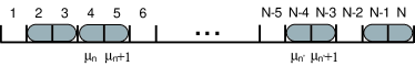
Figure 2: A schematic illustration of the randomly distributed brick model, used to explain the maximum number of independent Lyapunov vectors with only two non-zero particle components. The box labelled $j$ corresponds to the Lyapunov vector component of the $j$-th particle ($j=1,2,\cdots,N)$. Gray-filled rectangular bricks occupying boxes $\mu_{n}$ and $\mu_{n}+1$ represent possible non-zero components of Lyapunov vectors for which $n<n_{c}$. The value $n_{c}$ is the average number of bricks that can be randomly arranged on the set of boxes.

This situation is explained using a simple model whose schematic illustration is given in Fig. 2. In this randomly distributed brick model, N boxes corresponding to each of the particles are arranged on a line. Each Lyapunov vector represented by Eq. (5) must have non-zero components for only two particles $\delta\mbox{\boldmath$\bf\Gamma$}_{\mu_{n}}^{(n)}$ and $\delta\mbox{\boldmath$\bf\Gamma$}_{\mu_{n}+1}^{(n)}$. These are shown as a gray-filled rectangular brick filling boxes $\mu_{n}$ and $(\mu_{n}+1)$ in Fig. 2. To satisfy condition [I], these bricks must not overlap. The critical value $n_{c}$ is then the average number of bricks which can be put without overlaps on the $N$ different boxes.

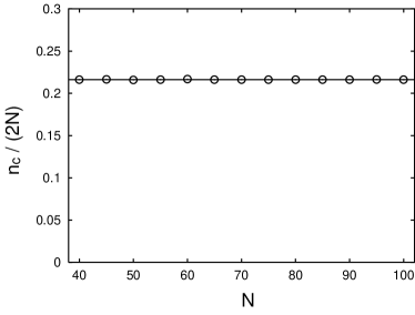
Figure 3: The normalized critical value $n_{c}/(2N)$ given by the randomly distributed brick model as a function of the number of particles $N$. The solid line is given by fitting the numerical data to a constant function $n_{c}/(2N)=\xi$ with the fitting parameter $\xi\approx 0.216$.

There is one more important point to get an explicit value of $n_{c}$ from the above mechanism:

[III]

The particle number $\mu_{n}$ in Eq. (5) is chosen randomly with respect to the Lyapunov index $n(<n_{c})$, so that there is no overlap among the non-zero Lyapunov vector components for Lyapunov vectors with different Lyapunov indices.

This means that the bricks shown in Fig. 2 must be randomly distributed without overlaps. Therefore randomly constructed configurations with any number of single empty boxes at non-neighboring positions are possible. Taking an ensemble average of the values of $\tilde{n}_{c}$ for each possible configuration we obtain the critical value $n_{c}$. Figure 3 shows the normalized critical value $n_{c}/(2N)$ from such a numerical simulation for different numbers of particles $N$. The data in this figure shows that $n_{c}/(2N)$ is independent of $N$, giving an estimate of the normalized critical value as

$$\frac{n_{c}}{2N}\approx 0.216.$$ (6)

The accuracy of this value can be used as a check of the proposed mechanism for the bending behavior of Lyapunov localization spectra at low density.

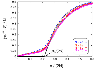
Figure 4: (Color online) The normalized Lyapunov localization spectra $\{(\mathcal{W}^{(n)}-2)/N\}_{n}$ as functions of the normalized Lyapunov index $n/(2N)$ in quasi-one-dimensional systems of different size; $N=40$ (diamonds), $N=50$ (triangles), $N=60$ (inverted triangles), and $N=70$ (squares) for a density given by $d=10000$. The lines are the asymptotic forms of Lyapunov localization spectra in the low density limit for these different values of $N$.

To draw the solid line shown in Fig. 1 we have already used the value obtained in Eq. (6). The parameters $\alpha$ and $\beta$ in Eq. (4) are regarded as fitting parameters, and we used values of $(\alpha,\beta)\approx(2.51,7.26)$ for the line in Fig. 1. The result shown in Fig. 1, using the critical value (6) gives a very satisfactory fit.

In order to check that the result (6) is satisfied for any number of particles $N$, we present Fig. 4. It is the $[n/(2N)]$-dependence of $[\mathcal{W}^{(n)}-2]/N$ in quasi-one-dimensional systems of different sizes at the same density. Notice that values of $[\mathcal{W}^{(n)}-2]/N$ themselves decrease slightly as the number of particles increases, meaning that the fitting parameters $\alpha$ and $\beta$ in Eq. (4) depend only slightly on $N$. The values of the fitting parameters $\alpha$ and $\beta$ for Fig. 4, were $(\alpha,\beta)\approx(2.83,7.83)$ for $N=40$ (dotted broken line), $(\alpha,\beta)\approx(2.51,7.26)$ for $N=50$ (dotted line), $(\alpha,\beta)\approx(2.28,6.80)$ for $N=60$ (broken line), and $(\alpha,\beta)\approx(2.10,6.39)$ for $N=70$ (solid line). However, all the data for different numbers of particles in Fig. 4 are nicely fitted using the same critical value $n_{c}/(2N)$, given by Eq. (6).

To conclude, we have shown that a model of randomly distributed bricks on a line (Fig. 2) can predict the maximum number of Lyapunov vectors which have a Lyapunov localization equal to two, in the low density limit. These are the Lyapunov vectors for which $n<n_{c}$ in the linear region that lead to the bending behavior of Lyapunov localization spectra. We showed that this behavior comes from a restriction on the maximum number of the most localized Lyapunov vectors with non-zero components for only two particles. The randomly distributed brick model was applied to quasi-one-dimensional systems, giving the specific value $n_{c}/(2N)\approx 0.216$ for the critical value $n_{c}$ of the Lyapunov localization spectra for any number of particles $N$. Numerical simulations give a value of $n_{c}/(2N)\approx 0.22\pm 0.06$. Our explanation for the bending behavior is independent of the system width $L_{y}$, as long as the particle order is invariant and the system remains quasi-one-dimensional. We have checked this using $L_{y}=2R(2-10^{-6})$ and the critical value is unchanged.

The critical value of Lyapunov localization spectra depends upon the shape of the system. Numerical results show that the critical value of the Lyapunov localization spectra for a square system is smaller than that for the quasi-one-dimensional system Tan03b . The randomly distributed brick model is specific to the quasi-one-dimensional system and would need to be generalized for a square system, and property [IIB]  can no longer be assumed. The calculation of the critical value $n_{c}$ for a general two (or three) dimensional systems remains as a future problem.

The authors appreciate the financial support by the Japan Society for the Promotion Science.

References

- (1) U. Dressler, Phys. Rev. A 38, 2103 (1988).
- (2) D. J. Evans and G. P. Morriss, Statistical mechanics of non-equilibrium liquids (Academic Press, 1990).
- (3) C. P. Dettmann and G. P. Morriss, Phys. Rev. E 53, R5545 (1996).
- (4) T. Taniguchi and G. P. Morriss, Phys. Rev. E 66, 066203 (2002).
- (5) H. A. Posch and R. Hirschl, in Hard ball systems and the Lorentz gas, edited by D. Szász (Springer, Berlin, 2000), p. 279.
- (6) J. -P. Eckmann and O. Gat, J. Stat. Phys. 98, 775 (2000).
- (7) T. Taniguchi and G. P. Morriss, Phys. Rev. E 65, 056202 (2002).
- (8) T. Taniguchi and G. P. Morriss, Phys. Rev. E 68, 026218 (2003).
- (9) M. Mareschal and S. McNamara, Physica D 187, 311 (2004).
- (10) A. S. de Wijn and H. van Beijeren, Phys. Rev. E 70, 016207 (2004).
- (11) H. Yang and G. Radons, e-print nlin.CD/0404027.
- (12) T. Taniguchi and G. P. Morriss, Phys. Rev. E 71, 016218 (2005).
- (13) C. Forster and H. A. Posch, e-print nlin.CD/0409019.
- (14) T. Taniguchi and G. P. Morriss, e-print nlin.CD/0404052.
- (15) P. Manneville, Lecture Note in Physics, 230, 319 (1985).
- (16) R. Livi and S. Ruffo, in Nonlinear Dynamics, edited by G. Turchetti (World Scientific, Singapore, 1989), p. 220.
- (17) K. Kaneko, Physica D 23, 436 (1986).
- (18) M. Falcioni, U. M. B. Marconi, and A. Vulpiani, Phys. Rev. A 44, 2263 (1991).
- (19) G. Giacomelli and A. Politi, Europhys. Lett. 15, 387 (1991).
- (20) A. Pikovsky and A. Politi, Nonlinearity 11, 1049 (1998).
- (21) A. Pikovsky and A. Politi, Phys. Rev. E 63, 036207 (2001).
- (22) Lj. Milanović and H. A. Posch, J. Mol. Liquids, 96-97, 221 (2002).
- (23) T. Taniguchi and G. P. Morriss, Phys. Rev. E 68 (2003) 046203.
- (24) In the normalized form of Lyapunov localization spectrum, its minimum value depends on . To effectively compare Lyapunov localization spectra with different numbers of particles, we use the normalized Lyapunov localization spectra minus in Figs. 1 and 2. This is crucial in Fig. 2 where the particle number dependence of Lyapunov localization spectra is discussed.