Stability Properties of Nonhyperbolic Chaotic Attractors under Noise

Abstract

We study local and global stability of nonhyperbolic chaotic attractors contaminated by noise. The former is given by the maximum distance of a noisy trajectory from the noisefree attractor, while the latter is provided by the minimal escape energy necessary to leave the basin of attraction, calculated with the Hamiltonian theory of large fluctuations. We establish the important and counterintuitive result that both concepts may be opposed to each other. Even when one attractor is globally more stable than another one, it can be locally less stable. Our results are exemplified with the Holmes map, for two different sets of parameter, and with a juxtaposition of the Holmes and the Ikeda maps. Finally, the experimental relevance of these findings is pointed out.

PACS numbers: 05.45.Gg, 02.50.-r, 05.20.-y, 05.40.-a

Noise plays an important role in nonlinear systems. Specifically, the fundamental question of the effect of noise on the stability of a chaotic attractor can be viewed under two different angles. The first aspect is to consider the escape from an attractor through random fluctuations. This is termed global stability. Relevant examples range from switching in lasers Hales:2000 , Penning traps Lapidus:1999 , over chemical reactions Gillespie:1977 to electronic circuits Luchinsky:1997 . Since the seminal work of Kramers Kramers:1940 , this problem has been treated for a broad range of settings Hanggi:1990 . For nonequilibrium systems, a WKB-like extension of Kramers’ equilibrium theory has been devised Onsager:1953 ; Freidlin:1984 . This so-called Hamiltonian theory of large fluctuations uses an approach similar to path integrals, thus obtaining the most probable exit path (MPEP). The MPEP, with an exponentially favoured probability of occurrence, yields in turn the optimal fluctuations and the minimal escape energy as well.
This theory has been employed for the calculation of the escape from a periodic state Kautz:1987 ; Beale:1989 ; Grassberger:1989 ; Dykman:1990 ; Silchenko:2003 . Recently, it has also become possible to treat the escape from a nonhyperbolic chaotic attractor (NCA) Kraut:2004 , whose stable and unstable manifolds exhibit tangencies. It was demonstrated that the MPEP is uniquely determined by the primary homoclinic tangency (PHT) closest to the basin boundary. A tangency is homoclinic if both manifolds belong to the same periodic orbit and primary, if a perturbation is amplified under forward and backward iteration of the dynamics. Since, in practice, virtually all chaotic attractors appear to be nonhyperbolic, it can be considered as the general case.
The second aspect of noise effects on NCAs is local stability, which is a measure of the maximum distance of a noisy trajectory from the noisefree attractor. Here, the trajectory is always close to the attractor, without leaving its basin of attraction. The concept of local stability of a NCA against noise is of fundamental importance and has bearings, e.g., on noise reduction Hammel:1990 , reconstruction of dynamical quantities Kostelich:1993 , parameter estimation McSharry:1999 , noise level evaluation Heald:2000 , and communication with chaos Bollt:1997 . When applying noise bounded by $\sigma$, for hyperbolic attractors the maximum distance scales as $\delta_{max}\sim\sigma$ Ott:1985 . For NCAs, however, it was shown that there is a much larger $\delta_{max}$ as compared to the hyperbolic case Jaeger:1997 , caused by attractor elongating deformations along the PHT and their images (see Schroer:1998 ; Kantz:2002 , as well). This was also confirmed experimentally Diestelhorst:1999 .
In this Letter we contrast these two measures of stability. While it is usually assumed that they behave in a similar fashion, we point here out, however, the counterintuitive effect that a nonhyberpolic chaotic attractor can be, in the above defined sense, globally more stable than another one, yet locally less stable. This is all the more surprising as both stability properties are intimately related to the primary homoclinic tangency. This phenomenon can be understood, though, by taking into account that for global stability the preimages are most relevant, constituting the proper and unique initial conditions for the most probable exit path Kraut:2004 . On the other hand, for local stability only the images govern the process Jaeger:1997 , as their local expansion rates, given by Eq. (2) below, contribute to a divergence from the attractor. Consequently, for local stability only linear properties of the system are relevant, whereas global stability can only be fully described by the complete set of variational equations, which are nonlinear.
We illustrate these findings first with the Holmes map Holmes:1979 with two different sets of parameters. Thereafter, we demonstrate this phenomenon by comparing the Holmes and the Ikeda map Ikeda:1979 . Since the Hamiltonian theory of large fluctuations is only valid for Gaussian noise and the maximum distance is only well defined for bounded noise, we calculate for local stability also the averaged Gaussian distance, including higher moments. This removes any particularity of comparing different noise distributions. The outcome of the calculation corroborates our main claim, too.
As a fundamental dynamical example we consider the Holmes map Holmes:1979

$$\begin{split}x_{n+1}&=\,y_{n}+\xi_{x}&\\ y_{n+1}&=\,a\,x_{n}+b\,y_{n}-c\,y_{n}^{3}+\xi_{y},&\end{split}$$ (1)

with the white noise terms $\xi_{x},\xi_{y}$ uniformly distributed in the disk $\sigma$: $\xi_{x}^{2}+\xi_{y}^{2}\leq\sigma$. We choose the first set of parameters to be (i) $a=0.047$, $b=2.4$ and $c=0.155$. That gives two attractors, symmetrical with respect to the origin; we focus only on one of these. When increasing $b$, these attractors merge in a crisis. Our second set of parameters is then in the region, where only one large symmetric chaotic attractor exists, (ii) $a=0.01$, $b=2.8$ and $c=0.8$. Both NCAs are normalized in a twofold way. First, the extensions in phase space $E=\sqrt{(x_{max}-x_{min})(y_{max}-y_{min})}$ are demanded to be the same, because then the percentage of noise on each attractor is identical. This is a common measure of the relative noise intensity, in turn adjusting the local properties. Second, the threshold of escape from the NCAs with bounded noise is also required to be equal. This guarantees the same scaling region for the maximum distance and calibrates the global properties. For the chosen parameters, the two measures yield $E\approx 3.1$ and $\sigma_{escape}\approx 0.13$ footnote1 . With these two conditions met, the comparison is as general and unambiguous as possible.
Let $\delta_{k}$ be at each step of iteration the minimum distance of the noisy trajectory from the noiseless attractor. The maximum distance $\delta_{max}$ of the whole trajectory is then defined as the maximum over all the minimum distances: $\delta_{max}=\underset{k}{\max}\,(\delta_{k})$. For the numerical computation, we partition the attractor with a grid of box edge length $l$, where $l$ depends on the noise strength and the desired resolution ($0.0005\leq l\leq 0.01$). We store only a limited number of points of the noiseless attractor per box of the grid (ca. 100). Each point of the noisy trajectory is then compared solely to attractor points of the box it falls in and the neighboring ones. If they are empty, the number of neighbors is increased until a point of the attractor has been encountered. This provides, for each trajectory point, the minimum distance from the attractor $\delta_{k}$, and the largest of these is $\delta_{max}$. With this method we get a much better accuracy and a larger scaling region than in Schroer:1998 ; Kantz:2002 , while simultaneously saving storage and computation time.
The result of the calculation for the two NCAs is shown in Fig. 1. The scaling is limited for small noise by our computational resolution and for large noise by the trajectory escaping from the attractor. It is apparent from the graph that, for all noise intensities, set (i) (circles) exhibits a larger $\delta_{max}$ than set (ii) (squares), indicating that the attractor (ii) is locally more stable than (i).

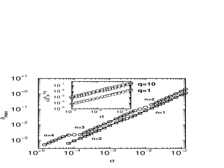
Figure 1: Maximum distance $\delta_{max}$ versus noise intensity $\sigma$ for the Holmes map, with the parameters (i) $a=0.047$, $b=2.4$ and $c=0.155$ (circles) and (ii) $a=0.01$, $b=2.8$ and $c=0.8$ (squares). The regions of linear growth are fitted by straight lines and marked with the number $n$ of the corresponding image of the PHT. For each noise strength $5\times 10^{9}$ iterations have been used. The inset shows the average $\langle\delta^{q}\rangle^{1/q}$, $q=1,10$, with Gaussian noise for set (i) (circles) and set (ii) (squares). $10^{9}$ iterations for each noise level have been averaged over.

The two curves in the log-log scale of Fig. 1 are straight lines, interrupted by bends. Between two bends, they have an identical slope 1 (i.e. $\delta_{max}=P_{n}\,\sigma$). The factor of proportionality $P_{n}$ varies with $n$, causing a different offset. The $\delta_{k}$ achieve their maxima at the PHT and images thereof (see Fig. 5 of Jaeger:1997 for a very instructive illustration). At the $n-th$ image, a perturbation at the PHT grows like Jaeger:1997

$$P_{n}=\sum_{i=0}^{n-1}\left|\prod_{j=1}^{n-i}\{Df[f^{i-1+j}({\bf x})]\}{\bf e}_{n-i}^{me}[f^{j}({\bf x})]\right|+1,$$ (2)

where $f({\bf x})$ is the dynamics of the system at ${\bf x}$, $Df({\bf x})$ the Jacobian, and ${\bf e}_{n-i}^{me}[f^{j}({\bf x})]$ the most expanding unit vector at $f^{j}({\bf x})$ under the application of $Df^{n-i}({\bf x})$. This factor sums up all the maximal stretching factors of the PHT and its images up to the $n-th$ one. Typically, $P_{n}>P_{m}$ for $n>m$, implying that the distance from the attractor increases with the number of images. However, because higher images are folded back on the attractor, other parts of the attractor instead of an iteration of the PHT come closer to the noisy trajectory as the noise level is incremented. This results in a saturation of the maximum distance, which produces a bend. In turn, when the noise strength is further augmented, $\delta_{max}$ switches to the next lower image of the PHT, again initiating a regime of linear growth, and so on.
In Fig. 1, the sequences $4\rightarrow 3\rightarrow 2$ for set (i) and $2\rightarrow 1$ for set (ii) can be seen. For set (ii), the offsets from the numerics of Fig. 1 for $n=1,2$ are $8.3,9.5$ (solid lines), while Eq. (2) yields $P_{n}=8.2,9.5$, a very good agreement. Set (i) for $n=2,3,4$ gives $15,17,34$ from Fig. 1 (solid lines), whereas Eq. (2) results in $P_{n}=13.4,16,34$, also a reasonably good agreement. The values for lower images of the PHT (i. e. higher noise) fit slightly worse. However, the matching can be improved by using the full dynamics instead of the linearized Eq. (2), since nonlinear effects play an increasing role for larger noise levels. By doing this, one gets $14.5,16.5,34$, again in good accordance.
To provide a better basis for the comparison with global stability, we calculate the averaged moments of the distance $\langle\delta^{q}\rangle^{1/q}$ = $(\frac{1}{N}\sum_{k=1}^{N}(\delta_{k})^{q})^{1/q}$ using Gaussian white noise, with $\langle\xi_{i}\rangle=0$ and $\langle\xi_{i},\xi_{j}\rangle=\sigma^{2}\,\delta_{ij}$. This is shown in Fig. 1, inset, for $q=1,10$. The corresponding moments for set (i) are for all $q$ above the ones of set (ii), more distinctive for higher q. The same applies for $\langle\delta^{q}\rangle^{1/q}$ with bounded noise (not shown). Here, in the limit $q\rightarrow\infty$ the maximum distance is recovered $\langle\delta^{q}\rangle^{1/q}\rightarrow\delta_{max}$.
Global stability is evaluated with the Hamiltonian theory of large fluctuations, solving a variational equation for the MPEP Grassberger:1989 ; Dykman:1990 ; Silchenko:2003 , which provides the action $S=\frac{1}{2}\sum_{n=1}^{N}{\bf\lambda_{n}^{T}}\,{\bf\lambda_{n}}$, with ${\bf\lambda_{n}}$ the optimal fluctuations. The mean first exit time is then given by $\langle\tau\rangle\sim\exp\left[\frac{S}{\sigma^{2}}\right]$. The MPEP starts at the preimages of the PHT, leaves the attractor close to the PHT and moves along their images towards the saddle point on the basin boundary Kraut:2004 . Employing this scheme, one obtains for set (i) $S\approx 0.015$ and for set (ii) $S\approx 0.01$, meaning now that set (i) is globally more stable than set (ii). We stress that this leads, e.g. for a noise value of $\sigma^{2}=0.001$, to an amplification of $\langle\tau\rangle$ by a factor of $\exp\left[\frac{0.005}{\sigma^{2}}\right]\approx 148$, it is therefore no small effect.
These opposing stability properties establish our main result. The Holmes map (as a typical example of a NCA) is with set (i) of parameters locally less stable than with set (ii), i.e., the maximum distance $\delta_{max}$ is larger, but globally more stable, i.e., the escape energy and consequently the mean first exit time are larger.

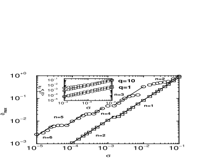
Figure 2: Maximum distance $\delta_{max}$ versus noise level $\sigma$ for the Ikeda and the Holmes maps, with the parameters (Ikeda) $a=0.9,b=0.9,\kappa=0.3$, and $\eta=6.0$ (circles) and set (iii) $a=0.01$, $b=2.78$ and $c=1.56$ (squares). For each noise strength $5\times 10^{9}$ iterations have been used. The inset shows the average $\langle\delta^{q}\rangle^{1/q}$, $q=1,10$, with Gaussian noise for Ikeda (circles) and set (iii) (squares). $10^{9}$ iterations for each noise level have been averaged over.

Next we demonstrate that this phenomenon can be much more pronounced when comparing two NCAs originating from different dynamical systems. For that purpose, we introduce the Ikeda map Ikeda:1979

$${\bf z_{n+1}}=a+b\,{\bf z_{n}}\exp\left[i\kappa-\frac{i\eta}{1+|{\bf z_{n}}|^{2}}\right]+{\bf\xi_{n}},$$ (3)

where ${\bf z_{n}}=x_{n}+iy_{n}$. We fix the parameters at $a=0.9,b=0.9,\kappa=0.3$ and $\eta=6.0$, which results in a NCA. We compare this NCA with the one obtained for the Holmes map with the parameter set (iii) $a=0.01$, $b=2.78$ and $c=1.56$. Again both attractors are normalized in the two ways explained above, with $E\approx 2.1$ and $\sigma_{escape}\approx 0.1$ footnote2 . The maximum distance is depicted in Fig. 2. The features are more striking than in the previous example, $\delta_{max}$ differs, for instance, for $\sigma=10^{-4}$, by one order of magnitude. Furthermore, the scenario of jumping from one image of the PHT to the next one happens for the Ikeda map more frequently. For the lowest noise level considered, the maximum distance occurs at the $6-th$ image of the PHT.
For set (iii) of the Holmes map, the numerical offsets of Fig. 2 (solid lines) come about as $8.2,11$ for the images $n=1,2$ of the PHT. Equation (2) results in $P_{n}=8,11.25$, agreeing extremely well. The Ikeda map gives for $n=2,3,4,5,6$ the numerical values $10,33,53,95,225$, respectively, while evaluated with Eq. (2) produces $P_{n}=8,22,50,96,247$. Taken into account that on the one hand for large images of the PHT the maximal distance is numerically hard to observe, as several subsequent optimal fluctuations are needed to achieve it, and on the other hand for low images the noise is already so large as to cause nonlinear effects, the correspondence is tolerably good.
In the inset of Fig. 2, the averaged distances with Gaussian noise $\langle\delta^{q}\rangle^{1/q},q=1,10$ are displayed. For small $q$ the Holmes map is here above the Ikeda map. This is rooted in the fact that the unstable manifold of the Ikeda map is more curved at the PHT and their images. Hence, the average exhibits less of the maximal possible expansion. However, for larger $q$ ($q=10$ in the graph), the average is above for all noise levels. Again, the same holds for $\langle\delta^{q}\rangle^{1/q}$ and bounded noise (not shown).
Global stability analysis, as before, entails for the Ikeda map $S\approx 0.025$ and for the parameter set (iii) of the Holmes map $S\approx 0.007$. Consequently, for the selected parameters, the Ikeda map is globally much more stable than the Holmes map, while it is locally much less stable, which is caused by the higher images of the PHT having larger expansion factors [Eq. (2)] and at the same time weaker folding back to the attractor. Both effects are most pronounced in the relevant low noise limit. The Ikeda map is globally more stable by a factor of $\exp\left[\frac{0.018}{\sigma^{2}}\right]$. The amplification becomes huge for small noise (e.g. $6.5\times 10^{7}$ for $\sigma^{2}=0.001$) and is easily measurable. This establishes that the phenomenon of opposite stability properties, when comparing NCAs originating from different dynamical models, can be observed in an even more striking manner.
We have confirmed this counterintuitive phenomenon also when comparing the Hénon map with both, the Ikeda and the Holmes maps, corroborating our findings, which we claim to be a general feature of NCAs.
In the present work, we were not concerned with the overall scaling of $\delta_{max}$, only with the fact that one curve lies above another, thus implying being locally less stable. In Schroer:1998 , however, it was claimed that the scaling is $\delta_{max}\sim\sigma^{\gamma}$, were $\gamma=1/D_{1}$, with $D_{1}$ the information dimension of the attractor. The agreement between this value and our, very accurate, numerics, is not too good, though footnote3 . This discrepancy is caused by the fact that in the derivation of the scaling in Schroer:1998 not $P_{n}$ from Eq. (2) was used, but the positive Lyapunov exponent, which usually has a smaller value. Thus, in general $1/D_{1}$ can be regarded only as a lower bound for $\gamma$. The question of an exact scaling exponent will be treated in Kraut:2005 .
As our findings can have an huge effect on the maximum distance and the average escape time, they have also relevance for experiments, since one cannot simply and straightforwardly conclude the behavior of one of the stability types by measuring the other.
We acknowledge D. G. Luchinsky, S. Beri, A. Pikovsky, M. S. Baptista, K. M. Zan, R. D. Vilela, A. E. Motter, and H. Kantz for valuable hints and discussions. This work was supported by the Alexander von Humboldt Stiftung, CNPq, and FAPESP.

References

- (1) J. Hales et al., Phys. Rev. Lett. 85, 78 (2000). (2000).
- (2) L. J. Lapidus, D. Enzer, and G. Gabrielse, Phys. Rev. Lett. 83, 899 (1999).
- (3) D. T. Gillespie, J. Chem. Phys. 81, 2340 (1977).
- (4) D. G. Luchinsky and P. V. E. McClintock, Nature (London) 389, 463 (1997).
- (5) H. A. Kramers, Physica (Utrecht) 7, 284 (1940).
- (6) P. Hänggi, P. Talkner, and M. Borkovec, Rev. Mod. Phys. 62, 251 (1990); V. I. Mel’nikov, Phys. Rep. 209, 1 (1991).
- (7) L. Onsager and S. Machlup, Phys. Rev. 91, 1505 (1953).
- (8) M. I. Freidlin and A. D. Wentzell, Random perturbations of dynamical systems, Springer Verlag, Berlin, 1984.
- (9) R. L. Kautz, Phys. Lett. A 125, 315 (1987).
- (10) P. D. Beale, Phys. Rev. A 40, 3998 (1989).
- (11) P. Grassberger, J. Phys. A 22, 3283 (1989).
- (12) M. I. Dykman, Phys. Rev. A 42, 2020 (1990).
- (13) A. N. Silchenko et al., Phys. Rev. Lett. 91, 174104 (2003).
- (14) S. Kraut and C. Grebogi, Phys. Rev. Lett. 92, 234101 (2004).
- (15) S. M. Hammel, Phys. Lett. A 148, 421 (1990); J. D. Farmer and J. J. Sidorowich, Physica (Amsterdam) 47D, 373 (1991); M. E. Davies, Chaos 8, 775 (1998).
- (16) E. J. Kostelich and T. Schreiber, Phys. Rev. E 48, 1752 (1993); C. L. Bremer and D. T. Kaplan, Physica (Amsterdam) 160D, 116 (2001).
- (17) P. E. McSharry and L. A. Smith, Phys. Rev. Lett. 83, 4285 (1999); R. Meyer and N. Christensen, Phys. Rev. E 62, 3535 (2000).
- (18) J. P. M. Heald and J. Stark, Phys. Rev. Lett. 84, 2366 (2000); M. Siefert et al., Europhys. Lett. 61, 466 (2003); K. Urbanowicz and J. A. Holyst, Phys. Rev. E 67, 046218 (2003).
- (19) E. Bollt, Y.-C. Lai, and C. Grebogi, Phys. Rev. Lett. 79, 3787 (1997); M. Dolnik and E. Bollt, Chaos 8, 702 (1998).
- (20) E. Ott, E. D. Yorke, and J. A. Yorke, Physica (Amsterdam) 16D, 62 (1985).
- (21) L. Jaeger and H. Kantz, Physica (Amsterdam) 105D, 79 (1997).
- (22) C. G. Schroer, E. Ott, and J. A. Yorke, Phys. Rev. Lett. 81, 1397 (1998).
- (23) H. Kantz et al., Phys. Rev. E 65, 026209 (2002).
- (24) M. Diestelhorst et al., Phys. Rev. Lett. 82, 2274 (1999).
- (25) P. Holmes, Philos. Trans. R. Soc. London A 292, 419 (1979).
- (26) K. Ikeda, Opt. Commun. 30, 257 (1979); S. M. Hammel, C. K. R. T. Jones, and J. V. Maloney, J. Opt. Soc. Am. B 2, 552 (1985).
- (27) For the symmetric case, we only consider half of the attractor for the calculation of , since it appears to be a more natural way to compare it with the other, asymmetric one. However, if one wants to take the entire attractor, one can choose the parameters , and . This yields again and . All other results remain qualitatively the same, as well.
- (28) Again, the same reasoning like in footnote1 applies. E.g. , and yields and , too, with all other conclusions equally valid.
- (29) We get for sets (i) and (ii) of Fig. 1 and , respectively, while and . For Fig. 2 we obtain for Ikeda and for set (iii), where and . The largest deviation is more than 10%.
- (30) S. Kraut, H. Kantz, C. Grebogi, (unpublished).